Chapter 1

Review

This chapter reviews notation and background material in mathematics, probability, and statistics. Readers may wish to skip this chapter and turn directly to Chapter 2, returning here only as needed.

1.1 Mathematical Notation

We use boldface to distinguish a vector x = (x₁, . . ., x_p) or a matrix M from a scalar variable x or a constant M. A vector-valued function f evaluated at x is also boldfaced, as in f(x) = (f₁(x), . . ., f_p(x)). The transpose of M is denoted M^T.

Unless otherwise specified, all vectors are considered to be column vectors, so, for example, an n × p matrix can be written as M = (x₁ . . . x_n)^T. Let I denote an identity matrix, and 1 and 0 denote vectors of ones and zeros, respectively.

A symmetric square matrix M is positive definite if x^TMx > 0 for all nonzero vectors x. Positive definiteness is equivalent to the condition that all eigenvalues of M are positive. M is nonnegative definite or positive semidefinite if x^TMx ≥ 0 for all nonzero vectors x.

The derivative of a function f, evaluated at x, is denoted f′(x). When x = (x₁, . . ., x_p), the gradient of f at x is

The Hessian matrix for f at x is f^′′(x) having (i, j)th element equal to d²f(x)/(dx_i dx_j). The negative Hessian has important uses in statistical inference.

Let J(x) denote the Jacobian matrix evaluated at x for the one-to-one mapping y = f(x). The (i, j)th element of J(x) is equal to df_i(x)/dx_j.

A functional is a real-valued function on a space of functions. For example, if , then the functional T maps suitably integrable functions onto the real line.

The indicator function 1_{A} equals 1 if A is true and 0 otherwise. The real line is denoted , and p-dimensional real space is .

1.2 Taylor's Theorem and Mathematical Limit Theory

First, we define standard “big oh” and “little oh” notation for describing the relative orders of convergence of functions. Let the functions f and g be defined on a common, possibly infinite interval. Let z₀ be a point in this interval or a boundary point of it (i.e., −∞ or ∞). We require g(z) ≠ 0 for all z ≠ z₀ in a neighborhood of z₀. Then we say

(1.1)

if there exists a constant M such that |f(z)| ≤ M|g(z)| as z → z₀. For example, , and it is understood that we are considering n→ ∞. If , then we say

(1.2)

For example, (h) as h → 0 if f is differentiable at x₀.The same notation can be used for describing the convergence of a sequence{x_n} as n→ ∞, by letting f(n) = x_n.

Taylor's theorem provides a polynomial approximation to a function f. Suppose f has finite (n + 1)th derivative on (a, b) and continuous nth derivative on [a, b]. Then for any x₀ [a, b] distinct from x, the Taylor series expansion of f about x₀ is

(1.3)

where is the jth derivative of f evaluated at x₀, and

(1.4)

for some point in the interval between x and x₀. As note that .

The multivariate version of Taylor's theorem is analogous. Suppose f is a real-valued function of a p-dimensional variable x, possessing continuous partial derivatives of all orders up to and including n + 1 with respect to all coordinates, in an open convex set containing x and . Then

(1.5)

where

(1.6)

and

(1.7)

for some on the line segment joining x and x₀. As , note that .

The Euler–Maclaurin formula is useful in many asymptotic analyses. If f has 2n continuous derivatives in [0, 1], then

(1.8)

where is the jth derivative of f, and bj = B_j(0) can be determined using the recursion relation

(1.9)

initialized with B₀(z) = 1. The proof of this result is based on repeated integrations by parts [376].

Finally, we note that it is sometimes desirable to approximate the derivative of a function numerically, using finite differences. For example, the ith component of the gradient of f at x can be approximated by

(1.10)

where is a small number and e_i is the unit vector in the ith coordinate direction. Typically, one might start with, say, or 0.001 and approximate the desired derivative for a sequence of progressively smaller . The approximation will generally improve until becomes small enough that the calculation is degraded and eventually dominated by computer roundoff error introduced by subtractive cancellation. Introductory discussion of this approach and a more sophisticated Richardson extrapolation strategy for obtaining greater precision are provided in [376]. Finite differences can also be used to approximate the second derivative of f at x via

(1.11)

with similar sequential precision improvements.

1.3 Statistical Notation and Probability Distributions

We use capital letters to denote random variables, such as Y or X, and lowercase letters to represent specific realized values of random variables such as y or x. The probability density function of X is denoted f; the cumulative distribution function is F. We use the notation X ~ f(x) to mean that X is distributed with density f(x). Frequently, the dependence of f(x) on one or more parameters also will be denoted with a conditioning bar, as in f(x|α, β). Because of the diversity of topics covered in this book, we want to be careful to distinguish when f(x|α) refers to a density function as opposed to the evaluation of that density at a point x. When the meaning is unclear from the context, we will be explicit, for example, by using f(· |α) to denote the function. When it is important to distinguish among several densities, we may adopt subscripts referring to specific random variables, so that the density functions for X and Y are f_X and f_Y, respectively. We use the same notation for distributions of discrete random variables and in the Bayesian context.

The conditional distribution of X given that Y equals y (i.e., X|Y = y) is described by the density denoted f(x|y), or f_X|Y(x|y). In this case, we write that X|Y has density f(x|Y). For notational simplicity we allow density functions to be implicitly specified by their arguments, so we may use the same symbol, say f, to refer to many distinct functions, as in the equation f(x, y|μ) = f(x|y, μ)f(y|μ). Finally, f(X) and F(X) are random variables: the evaluations of the density and cumulative distribution functions, respectively, at the random argument X.

The expectation of a random variable is denoted E{X}. Unless specifically mentioned, the distribution with respect to which an expectation is taken is the distribution of X or should be implicit from the context. To denote the probability of an event A, we use P[A] = E{1_{A}}. The conditional expectation of X|Y = y is E{X|y}. When Y is unknown, E{X|Y} is a random variable that depends on Y. Other attributes of the distribution of X and Y include var{X}, cov{X, Y}, cor{X, Y}, and cv. These quantities are the variance of X, the covariance and correlation of X and Y, and the coefficient of variation of X, respectively.

A useful result regarding expectations is Jensen's inequality. Let g be a convex function on a possibly infinite open interval I, so

(1.12)

for all x, y I and all 0 < λ < 1. Then Jensen's inequality states that E{g(X)} ≥ g(E{X}) for any random variable X having P[X I] = 1.

Tables 1.1, 1.2, and 1.3 provide information about many discrete and continuous distributions used throughout this book. We refer to the following well-known combinatorial constants:

(1.13)

(1.14)

(1.15)

(1.16)

Table 1.1 Notation and description for common probability distributions of discrete random variables.

Table 1.2 Notation and description for some common probability distributions of continuous random variables.

Table 1.3 Notation and description for more common probability distributions of continuous random variables.

It is worth knowing that

for positive integer n.

Many of the distributions commonly used in statistics are members of an exponential family. A k-parameter exponential family density can be expressed as

(1.17)

for nonnegative functions c₁ and c₂. The vector γ denotes the familiar parameters, such as λ for the Poisson density and p for the binomial density. The real-valued θ_i(γ) are the natural, or canonical, parameters, which are usually transformations of γ. The y_i(x) are the sufficient statistics for the canonical parameters. It is straightforward to show

(1.18)

and

(1.19)

where κ(θ) = − log c₃(θ), letting c₃(θ) denote the reexpression of c₂(γ) in terms of the canonical parameters θ = (θ₁, . . ., θ_k), and y(X) = (y₁(X), . . ., y_k(X)). These results can be rewritten in terms of the original parameters γ as

(1.20)

and

(1.21)

Example 1.1 (Poisson) The Poisson distribution belongs to the exponential family with c₁(x) = 1/x !, c₂(λ) = exp { − λ}, y(x) = x, and θ(λ) = log λ. Deriving moments in terms of θ, we have κ(θ) = exp {θ}, so E{X} = κ′(θ) = exp {θ} = λ and var{X} = κ^′′(θ) = exp {θ} = λ. The same results may be obtained with (1.20) and (1.21), noting that dθ/dλ = 1/λ. For example, (1.20) gives .

It is also important to know how the distribution of a random variable changes when it is transformed. Let X = (X₁, . . ., X_p) denote a p-dimensional random variable with continuous density function f. Suppose that

(1.22)

where g is a one-to-one function mapping the support region of f onto the space of all u = g(x) for which x satisfies f(x) > 0. To derive the probability distribution of U from that of X, we need to use the Jacobian matrix. The density of the transformed variables is

(1.23)

where is the absolute value of the determinant of the Jacobian matrix of g⁻¹ evaluated at u, having (i, j)th element dx_i/du_j, where these derivatives are assumed to be continuous over the support region of U.

1.4 Likelihood Inference

If X₁, . . ., X_n are independent and identically distributed (i.i.d.) each having density that depends on a vector of p unknown parameters θ = (θ₁, . . ., θ_p), then the joint likelihood function is

(1.24)

When the data are not i.i.d., the joint likelihood is still expressed as the joint density f(x₁, . . ., x_n|θ) viewed as a function of θ.

The observed data, x₁, . . ., x_n, might have been realized under many different values for θ. The parameters for which observing x₁, . . ., x_n would be most likely constitute the maximum likelihood estimate of θ. In other words, if is the function of x₁, . . ., x_n that maximizes L(θ), then is the maximum likelihood estimator (MLE) for θ. MLEs are invariant to transformation, so the MLE of a transformation of θ equals the transformation of .

It is typically easier to work with the log likelihood function,

(1.25)

which has the same maximum as the original likelihood, since log is a strictly monotonic function. Furthermore, any additive constants (involving possibly x₁, . . ., x_n but not θ) may be omitted from the log likelihood without changing the location of its maximum or differences between log likelihoods at different θ. Note that maximizing L(θ) with respect to θ is equivalent to solving the system of equations

(1.26)

where

is called the score function. The score function satisfies

(1.27)

where the expectation is taken with respect to the distribution of X₁, . . ., X_n. Sometimes an analytical solution to (1.26) provides the MLE; this book describes a variety of methods that can be used when the MLE cannot be solved for in closed form. It is worth noting that there are pathological circumstances where the MLE is not a solution of the score equation, or the MLE is not unique; see [127] for examples.

The MLE has a sampling distribution because it depends on the realization of the random variables X₁, . . ., X_n. The MLE may be biased or unbiased for θ, yet under quite general conditions it is asymptotically unbiased as n→ ∞. The sampling variance of the MLE depends on the average curvature of the log likelihood: When the log likelihood is very pointy, the location of the maximum is more precisely known.

To make this precise, let l^′′(θ) denote the p × p matrix having (i, j)th element given by d²l(θ)/(dθ_idθ_j). The Fisher information matrix is defined as

(1.28)

where the expectations are taken with respect to the distribution of X₁, . . ., X_n. The final equality in (1.28) requires mild assumptions, which are satisfied, for example, in exponential families. I(θ) may sometimes be called the expected Fisher information to distinguish it from −l^′′(θ), which is the observed Fisher information. There are two reasons why the observed Fisher information is quite useful. First, it can be calculated even if the expectations in (1.28) cannot easily be computed. Second, it is a good approximation to I(θ) that improves as n increases.

Under regularity conditions, the asymptotic variance–covariance matrix of the MLE is I(θ^∗)⁻¹, where θ^∗ denotes the true value of θ. Indeed, as n→ ∞, the limiting distribution of is N_p(θ^∗, I(θ^∗)⁻¹). Since the true parameter values are unknown, I(θ^∗)⁻¹ must be estimated in order to estimate the variance–covariance matrix of the MLE. An obvious approach is to use . Alternatively, it is also reasonable to use . Standard errors for individual parameter MLEs can be estimated by taking the square root of the diagonal elements of the chosen estimate of I(θ^∗)⁻¹. A thorough introduction to maximum likelihood theory and the relative merits of these estimates of I(θ^∗)⁻¹ can be found in [127, 182, 371, 470].

Profile likelihoods provide an informative way to graph a higher-dimensional likelihood surface, to make inference about some parameters while treating others as nuisance parameters, and to facilitate various optimization strategies. The profile likelihood is obtained by constrained maximization of the full likelihood with respect to parameters to be ignored. If θ = (μ, ϕ), then the profile likelihood for ϕ is

(1.29)

Thus, for each possible ϕ, a value of μ is chosen to maximize L(μ, ϕ). This optimal μ is a function of ϕ. The profile likelihood is the function that maps ϕ to the value of the full likelihood evaluated at ϕ and its corresponding optimal μ. Note that the that maximizes the profile likelihood is also the MLE for ϕ obtained from the full likelihood L(μ, ϕ). Profile likelihood methods are examined in [23].

1.5 Bayesian Inference

In the Bayesian inferential paradigm, probability distributions are associated with the parameters of the likelihood, as if the parameters were random variables. The probability distributions are used to assign subjective relative probabilities to regions of parameter space to reflect knowledge (and uncertainty) about the parameters.

Suppose that X has a distribution parameterized by θ. Let f(θ) represent the density assigned to θ before observing the data. This is called a prior distribution. It may be based on previous data and analyses (e.g., pilot studies), it may represent a purely subjective personal belief, or it may be chosen in a way intended to have limited influence on final inference.

Bayesian inference is driven by the likelihood, often denoted L(θ|x) in this context. Having established a prior distribution for θ and subsequently observed data yielding a likelihood that is informative about θ, one's prior beliefs must be updated to reflect the information contained in the likelihood. The updating mechanism is Bayes' theorem:

(1.30)

where f(θ|x) is the posterior density of θ. The posterior distribution for θ is used for statistical inference about θ. The constant c equals 1/∫ f(θ)L(θ|x)dθ and is often difficult to compute directly, although some inferences do not require c. This book describes a large variety of methods for enabling Bayesian inference, including the estimation of c.

Let be the posterior mode, and let θ^∗ be the true value of θ. The posterior distribution of converges to N(θ^∗, I(θ^∗)⁻¹) as n→ ∞, under regularity conditions. Note that this is the same limiting distribution as for the MLE. Thus, the posterior mode is of particular interest as a consistent estimator of θ. This convergence reflects the fundamental notion that the observed data should overwhelm any prior as n→ ∞.

Bayesian evaluation of hypotheses relies upon the Bayes factor. The ratio of posterior probabilities of two competing hypotheses or models, H₁ and H₂, is

(1.31)

where P[H_i|x] denotes posterior probability, P[H_i] denotes prior probability, and

(1.32)

with θ_i denoting the parameters corresponding to the ith hypothesis. The quantity B_2,1 is the Bayes factor; it represents the factor by which the prior odds are multiplied to produce the posterior odds, given the data. The hypotheses H₁ and H₂ need not be nested as for likelihood ratio methods. The computation and interpretation of Bayes factors is reviewed in [365].

Bayesian interval estimation often relies on a 95% highest posterior density (HPD) region. The HPD region for a parameter is the region of shortest total length containing 95% of the posterior probability for that parameter for which the posterior density for every point contained in the interval is never lower than the density for every point outside the interval. For unimodal posteriors, the HPD is the narrowest possible interval containing 95% of the posterior probability. A more general interval for Bayesian inference is a credible interval. The 100(1− α) % credible interval is the region between the α/2 and 1 − α/2 quantiles of the posterior distribution. When the posterior density is symmetric and unimodal, the HPD and the credible interval are identical.

A primary benefit of the Bayesian approach to inference is the natural manner in which resulting credibility intervals and other inferences are interpreted. One may speak of the posterior probability that the parameter is in some range. There is also a sound philosophical basis for the Bayesian paradigm; see [28] for an introduction. Gelman et al. provide a broad survey of Bayesian theory and methods [221].

The best prior distributions are those based on prior data. A strategy that is algebraically convenient is to seek conjugacy. A conjugate prior distribution is one that yields a posterior distribution in the same parametric family as the prior distribution. Exponential families are the only classes of distributions that have natural conjugate prior distributions.

When prior information is poor, it is important to ensure that the chosen prior distribution does not strongly influence posterior inferences. A posterior that is strongly influenced by the prior is said to be highly sensitive to the prior. Several strategies are available to reduce sensitivity. The simplest approach is to use a prior whose support is dispersed over a much broader region than the parameter region supported by the data, and fairly flat over it. A more formal approach is to use a Jeffreys prior [350]. In the univariate case, the Jeffreys prior is f(θ) ∝ I(θ)^−1/2, where I(θ) is the Fisher information; multivariate extensions are possible. In some cases, the improper prior f(θ) ∝ 1 may be considered, but this can lead to improper posteriors (i.e., not integrable), and it can be unintentionally informative depending on the parameterization of the problem.

Example 1.2 (Normal–Normal Conjugate Bayes Model) Consider Bayesian inference based on observations of i.i.d. random variables X₁, . . ., X_n with density X_i|θ ~ N(θ, σ²) where σ² is known. For such a likelihood, a normal prior for θ is conjugate. Suppose the prior is θ ~ N(μ, τ²). The posterior density is

(1.33)

(1.34)

(1.35)

where is the sample mean. Recognizing (1.35) as being in the form of a normal distribution, we conclude that , where

(1.36)

and

(1.37)

Hence, a posterior 95% credibility interval for θ is (μ_n − 1.96τ_n, μ_n + 1.96τ_n). Since the normal distribution is symmetric, this is also the posterior 95% HPD for θ.

For fixed σ, consider increasingly large choices for the value of τ. The posterior variance for θ converges to σ²/n as τ²→ ∞. In other words, the influence of the prior on the posterior vanishes as the prior variance increases. Next, note that

This shows that the posterior variance for θ and the sampling variance for the MLE, , are asymptotically equal, and the effect of any choice for τ is washed out with increasing sample size.

As an alternative to the conjugate prior, consider using the improper prior f(θ) ∝ 1. In this case, , and a 95% posterior credibility interval corresponds to the standard 95% confidence interval found using frequentist methods.

1.6 Statistical Limit Theory

Although this book is mostly concerned with a pragmatic examination of how and why various methods work, it is useful from time to time to speak more precisely about the limiting behavior of the estimators produced by some procedures. We review below some basic convergence concepts used in probability and statistics.

A sequence of random variables, X₁, X₂, . . ., is said to converge in probability to the random variable X if lim _n→∞P[|X_n − X| < ] = 1 for every > 0. The sequence converges almost surely to X if P[lim _n→∞|X_n − X| < ] = 1 for every > 0. The variables converge in distribution to the distribution of X if for all points x at which F_X(x) is continuous. The variable X has property A almost everywhere if P[A] = ∫ 1_{A}f_X(x)dx = 1.

Some of the best-known convergence theorems in statistics are the laws of large numbers and the central limit theorem. For i.i.d. sequences of one-dimensional random variables X₁, X₂, . . ., let . The weak law of large numbers states that converges in probability to μ = E{X_i} if E{|X_i|}< ∞. The strong law of large numbers states that converges almost surely to μ if E{|X_i|}< ∞. Both results hold under the more stringent but easily checked condition that var{X_i} = σ²< ∞.

If θ is a parameter and T_n is a statistic based on X₁, . . ., X_n, then T_n is said to be weakly or strongly consistent for θ if T_n converges in probability or almost surely (respectively) to θ. T_n is unbiased for θ if E{T_n} = θ; otherwise the bias is E{T_n} − θ. If the bias vanishes as n→ ∞, then T_n is asymptotically unbiased.

A simple form of the central limit theorem is as follows. Suppose that i.i.d. random variables X₁, . . ., X_n have mean μ and finite variance σ², and that E{ exp {tX_i}} exists in a neighborhood of t = 0. Then the random variable converges in distribution to a normal random variable with mean zero and variance one, as n→ ∞. There are many versions of the central limit theorem for various situations. Generally speaking, the assumption of finite variance is critical, but the assumptions of independence and identical distributions can be relaxed in certain situations.

1.7 Markov Chains

We offer here a brief introduction to univariate, discrete-time, discrete-state-space Markov chains. We will use Markov chains in Chapters 7 and 8. A thorough introduction to Markov chains is given in [556], and higher-level study is provided in [462, 543].

Consider a sequence of random variables , t = 0, 1, . . ., where each X^(t) may equal one of a finite or countably infinite number of possible values, called states. The notation X^(t) = j indicates that the process is in state j at time t. The state space, , is the set of possible values of the random variable X^(t).

A complete probabilistic specification of X⁽⁰⁾, . . ., X⁽ⁿ⁾ would be to write their joint distribution as the product of conditional distributions of each random variable given its history, or

(1.38)

A simplification of (1.38) is possible under the conditional independence assumption that

(1.39)

Here the next state observed is only dependent upon the present state. This is the Markov property, sometimes called “one-step memory.” In this case,

(1.40)

Let be the probability that the observed state changes from state i at time t to state j at time t + 1. The sequence , t = 0, 1, . . . is a Markov chain if

(1.41)

for all t = 0, 1, . . . and x⁽⁰⁾, x⁽¹⁾, . . ., x^(t−1), . The quantity is called the one-step transition probability. If none of the one-step transition probabilities change with t, then the chain is called time homogeneous, and . If any of the one-step transition probabilities change with t, then the chain is called time-inhomogeneous.

A Markov chain is governed by a transition probability matrix. Suppose that the s states in are, without loss of generality, all integer valued. Then P denotes s × s transition probability matrix of a time-homogeneous chain, and the (i, j)th element of P is p_ij. Each element in P must be between zero and one, and each row of the matrix must sum to one.

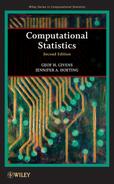
Example 1.3 (San Francisco Weather) Let us consider daily precipitation outcomes in San Francisco. Table 1.4 gives the rainfall status for 1814 pairs of consecutive days [488]. The data are taken from the months of November through March, starting in November of 1990 and ending in March of 2002. These months are when San Francisco receives over 80% of its precipitation each year, virtually all in the form of rain. We consider a binary classification of each day. A day is considered to be wet if more than 0.01 inch of precipitation is recorded and dry otherwise. Thus, has two elements: “wet” and “dry.” The random variable corresponding to the state for the tth day is X^(t).

Assuming time homogeneity, an estimated transition probability matrix for X^(t) would be

(1.42)

Clearly, wet and dry weather states are not independent in San Francisco, as a wet day is more likely to be followed by a wet day and pairs of dry days are highly likely.

Table 1.4 San Francisco rain data considered in Example 1.3.

	Wet Today	Dry Today
Wet Yesterday	418	256
Dry Yesterday	256	884

The limiting theory of Markov chains is important for many of the methods discussed in this book. We now review some basic results.

A state to which the chain returns with probability 1 is called a recurrent state. A state for which the expected time until recurrence is finite is called nonnull. For finite state spaces, recurrent states are nonnull.

A Markov chain is irreducible if any state j can be reached from any state i in a finite number of steps for all i and j. In other words, for each i and j there must exist m > 0 such that . A Markov chain is periodic if it can visit certain portions of the state space only at certain regularly spaced intervals. State j has period d if the probability of going from state j to state j in n steps is 0 for all n not divisible by d. If every state in a Markov chain has period 1, then the chain is called aperiodic. A Markov chain is ergodic if it is irreducible, aperiodic, and all its states are nonnull and recurrent.

Let π denote a vector of probabilities that sum to one, with ith element π_i denoting the marginal probability that X^(t) = i. Then the marginal distribution of X^(t+1) must be π^TP. Any discrete probability distribution π such that π^TP = π^T is called a stationary distribution for P, or for the Markov chain having transition probability matrix P. If X^(t) follows a stationary distribution, then the marginal distributions of X^(t) and X^(t+1) are identical.

If a time-homogeneous Markov chain satisfies

(1.43)

for all , then π is a stationary distribution for the chain, and the chain is called reversible because the joint distribution of a sequence of observations is the same whether the chain is run forwards or backwards. Equation (1.43) is called the detailed balance condition.

If a Markov chain with transition probability matrix P and stationary distribution π is irreducible and aperiodic, then π is unique and

(1.44)

where π_j is the jth element of π. The π_j are the solutions of the following set of equations:

(1.45)

We can restate and extend (1.44) as follows. If X⁽¹⁾, X⁽²⁾, . . . are realizations from an irreducible and aperiodic Markov chain with stationary distribution π, then X⁽ⁿ⁾ converges in distribution to the distribution given by π, and for any function h,

(1.46)

almost surely as n→ ∞, provided E_π{|h(X)|} exists [605]. This is one form of the ergodic theorem, which is a generalization of the strong law of large numbers.

We have considered here only Markov chains for discrete state spaces. In Chapters 7 and 8 we will apply these ideas to continuous state spaces. The principles and results for continuous state spaces and multivariate random variables are similar to the simple results given here.

1.8 Computing

If you are new to computer programming, or wishing to learn a new language, there is no better time to start than now. Our preferred language for teaching and learning about statistical computing is R (freely available at www.r-project.org), but we avoid any language-specific limitations in this text. Most of the methods described in this book can also be easily implemented in other high-level computer languages for mathematics and statistics such as MATLAB. Programming in Java and low-level languages such as C++ and FORTRAN is also possible. The tradeoff between implementation ease for high-level languages and computation speed for low-level languages often guides this selection. Links to these and other useful software packages, including libraries of code for some of the methods described in this book, are available on the book website.

Ideally, your computer programming background includes a basic understanding of computer arithmetic: how real numbers and mathematical operations are implemented in the binary world of a computer. We focus on higher-level issues in this book, but the most meticulous implementation of the algorithms we describe can require consideration of the vagaries of computer arithmetic, or use of available routines that competently deal with such issues. Interested readers may refer to [383].