
17
MS-EXCEL 2007
Contents
- Introduction
- Basics of spreadsheet
- Start MS-Excel
- MS-Excel screen and its components— Office logo button, quick access toolbar, ribbon, tabs, group, status bar, scroll bar, worksheet tab, row, column headings, active cell, formula bar, name box
- Office button—New, open, save, save As, print, prepare, send, publish, close
- Ribbon—Home, insert, page layout, formulas, data, review, view, add-ins
- Home tab—Clipboard, font, alignment, number, styles, cells, editing
- Insert tab—Tables, illustrations, charts, links, text
- Page layout tab—Themes, page setup, scale to fit, sheet options, arrange
- Formulas tab—Function library, defined names, formula auditing, calculation
- Data tab—Get external data, connections, sort and filter, data tools, outline
- The review tab—Proofing, comments, changes
- The view tab—Workbook views, show/ hide, zoom, window, macros
- The help
- Solved examples—Year-wise salesman sales, salary calculation, mark sheet calculation
Why this chapter
An electronic spreadsheet is used for analyzing, sharing and managing information for accounting purposes, performing mathematical calculations, budgeting, billing, report generation etc. Tools are included in the spreadsheet software to facilitate the creation of charts, graphs, data analysis etc. MS-Excel is commonly used electronic spreadsheet software. The purpose of this chapter is to introduce you to MS-Excel.
17.1 INTRODUCTION
A spreadsheet is a matrix of rows and columns, similar to an accounting notebook (ledger). A spreadsheet program is primarily used for mathematical calculations. A spreadsheet program is often used to prepare budgets, financial projections, billing, and other reports arranged in rows and columns. An electronic spreadsheet provides more flexibility, speed, and accuracy in comparison to a manually maintained spreadsheet. For example, if you change the numbers in a spreadsheet, you do not have to perform the calculations again. The spreadsheet does it for you. The spreadsheet program also provides tools for creating graphs, inserting pictures and chart, analyzing the data etc.
The spreadsheet software from different technology vendors are available for creation of spreadsheets. Apple Numbers, Microsoft Excel (MS-Excel), Corel Quattro Pro, and Lotus 1-2-3 are some of the spreadsheet software available in the market. Lotus 1-2-3 was the leading software when DOS was the predominant operating system. Several open-source spreadsheet software, like, Sun’s OpenOffice.org Calc, Google Docs, KSpread, and Gnumeric are also available. IBM Lotus Symphony is freeware spreadsheet software.
MS-Excel is the most commonly known spreadsheet software. It is part of the MS-Office suite, and runs on Microsoft Windows, and Mac OS X operating systems. In addition to MS-Excel, MS-Office suite contains other software like MS-Word, MS-PowerPoint and MS-Access. MS-Excel is GUI-based software. MS-Excel includes tools for analyzing, managing, and sharing information, which helps during the decision making process. The spreadsheet in MS-Excel may contain charts, text, and other objects. Some of the important features of MS-Excel are as follows:
- It allows organization, tabulation, search, and exploration of data of large sizes.
- Based on the values entered in different cells in the spreadsheet, formulas can be defined, which automatically perform calculations.
- It allows the design of professionally looking charts with 3-D effects, shadowing, and transparency.
- The tables can be easily created, formatted, expanded, and referred to within formulas.
- The data can be filtered and sorted.
- PivotTable views enable you to quickly re-orient your data to help you answer multiple questions.
- Formatting of spreadsheet allows changing the font size, font color, and font style.
- A function library consists of various function groups like financial, logical, math & trignometry etc. from which you can apply long and complex formulas.
- Conditional formatting can be applied to discover patterns and to highlight trends in the data.
This chapter discusses the using of the MS-Excel software in detail. There are many versions of the MS-Excel software. Here, we will discuss the MS-Excel 2007.
In this chapter, we use the following terminology while working with the mouse:
- Pointer —a mouse pointer
- Click—press left button of mouse once
- Double Click—press left button of mouse twice
- Select —move the pointer of mouse and keep the left button of the mouse pressed over the area that you want to select. The selected area will appear in a dark background.
- Quick Menu—Right click (press right button of mouse once) to get a quick menu.
The commands are enclosed in braces <Command> to represent the command to be clicked.
17.2 START MS-EXCEL
Figure 17.1 MS-Excel icon
The MS-Excel software for the Windows operating system should be installed on the computer. MS-Excel is a fully menu-driven software, and the commands are available as icons in various Tabs, and Groups. While working in MS-Excel, using a mouse makes working on MS– Excel simpler although one can work to some extent through the keyboard also.
To start using the MS-Excel software, any one of the following steps needs to be performed:
- If a shortcut key to MS-Excel is available as an icon on the Desktop, as shown in Figure 17.1, then double-click the icon, or
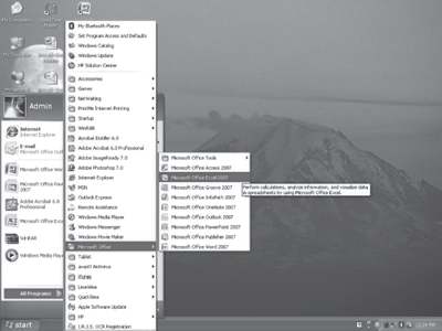
Figure 17.2 Start MS-Excel
- <Start> <All Programs> <Microsoft Office> <Microsoft Office Excel 2007>. (Figure 17.2)
17.3 BASICS OF SPREADSHEET
MS-Excel 2007 allows creation of spreadsheets. In this section, we will discuss the basics of spreadsheet (Figure 17.3).
- A spreadsheet is an electronic document that stores various types of data. There are vertical columns and horizontal rows.
- The intersection of each row and column is called a cell. A cell is named with the column letter first and then the row number. For example, cell A1, A2, B1, B3 etc. A cell is an individual container for data (like a box). A cell may hold data of the following types:
- Numbers (constants),
- Formulas (mathematical equations), and
- Text (labels).
- A cell can be used in calculations of data within the spreadsheet.
- An array of cells is called a sheet or worksheet. A spreadsheet or worksheet holds information presented in tabular row and column format with text that labels the data. They can also contain graphics and charts.
- A workbook is a Microsoft Office document that contains one or more worksheets. A worksheet is a single document inside a workbook. However, the terms workbook, worksheet, sheet, and spreadsheet are often used interchangeably.
- Each new workbook created in Excel has three worksheets by default. If you want to rename a worksheet, right click on the tab <Rename>, or double click on the tab and type the new name for it. User can add more worksheets or delete some of them, as per requirements.
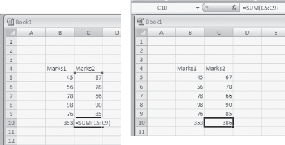
- A formula is an equation that calculates the value to be displayed. A formula when used in a worksheet, must begin with an equal to (=) sign. When using a formula, do not type the number you want to add, but the reference to the cells whose content you want to add. For example, to add the marks 67, 78, 66, 90, 85, and insert the result in C10 cell, you put the formula =SUM(C5:C9) in C10 cell, where C5 is the cell from where we want to start finding the sum, and C9 is the cell having the last data we want to add. After writing the formula, when you press the Enter key, cell C10 displays the result i.e. 386. The actual formula contained in the cell C10, gets displayed in the formula bar, when you click over the number 386. It is advisable to reference the cell as opposed to typing the data contained in the cell, into the formulas.
17.4 MS-EXCEL SCREEN AND ITS COMPONENTS
The user interface of the MS-Excel makes it easy to use Excel 2007. In contrast to the previous versions of MS-Excel, the new user-interface has an improved navigation system consisting of tabs which further consist of group of commands. The main screen is shown in Figure 17.3. At the top side of the screen is the Ribbon. Below the Ribbon are the Name box and the Formula box. There is a scroll bar, and at the lower side of the screen there are the Worksheet tabs and the Status Bar. The work area of the screen consists of rows and columns. The orientation of the Excel 2007 layout and its general features are described as follows:
- The Office Logo button
 at the top left corner contains many commands for the document such as, New, Open, Save, Save As, Print, and Close. This button also has a list of the recent documents. Some of these commands include an expandable menu to provide additional options. This Office Logo button replaces the File menu in the earlier versions of MS-Office.
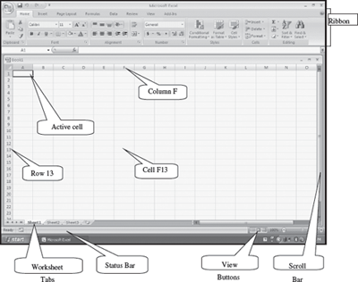
Figure 17.3 MS-Excel screen
- The Quick Access Toolbar
 is to the right of the Office Logo button. It contains shortcuts for the commonly used commands, like, Save
  Undo
Undo  (reverses the last change) and Repeat
  (repeats the last action). The icons for the commands that the user want to get displayed on the toolbar can be selected from the
  Customize Quick Access Toolbar

- The Ribbon consists of a panel of commands which are organized into a set of tabs (Figure 17.4). The layout of the Ribbon in MS-Excel is same as that of the Ribbon in MS– Word. Within Tabs are Groups, which are designated by the names located on the bottom of the Ribbon. Each group has icons for the associated command. The Ribbon (Tabs, Groups, and Icons) replaces the traditional toolbars and menus of earlier versions of MS-Excel.
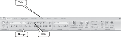
Figure 17.4 The ribbon
- The Tabs (Home, Insert etc.) on the Ribbon contain the commands needed to insert data, page layout, formulas etc. as well as any additional commands that you may need.

- Each Tab consists of different Groups, like the Home tab has seven groups namely, Clipboard, Font, Alignment, Number, Styles, Cells, and Editing.

- Each group has icons for the commands. To know the function of an icon (or command), leave the pointer on a button for a few seconds, the function of that icon will appear in a small box below the pointer. Forexample, leaving the icon on
 displays “Bold (Ctrl+B)”.
- Status Bar—It displays information about the currently active worksheet. The information includes the page number, view shortcuts, zoom slider
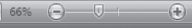 etc.Right-click on the status bar will show you the Customize Status bar (Figure 17.5) pop-up menu. You can select the options you want to view on the status bar.
 - Scroll Bar—There are two scroll bars—horizontal and vertical. They help to scroll the content or the body of worksheet. Scrolling is done by moving the elevator button along the scroll bar, or by clicking on the buttons with the arrow marked on them to move up and down, and left and right of a worksheet.
- Worksheet Tab—They are the tabs located at the bottom of
 each worksheet in the workbook, which display the names of the sheets. A button is provided to insert a new worksheet. You can move from one worksheet to other using the arrow keys or by clicking on the appropriate worksheet tab.

- Row—The numbers (1, 2, 3 …) that appear on the left side of the worksheet window. The rows are numbered consecutively starting from 1 to 1,048,576 (approx. 1 million rows).
- Column Headings—The letters that appear along the top of the worksheet window. Columns are listed alphabetically starting from A to XFD i.e.16,384, (approx.16,000 columns).
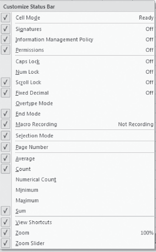
Figure 17.5 Customize status bar
- Active Cell—The intersection of a row and column is called a cell. The cell in which you are currently working is the active cell. A dark border outlining the cell identifies the active cell.
- Formula Bar—It is located beneath the Ribbon. Formula bar is used to enter and edit worksheet data. As you type or edit the data, the changes appear in the Formula Bar. When you click the mouse in the formula bar, an X and a check mark appear. You can click the check icon to confirm and complete editing, or the X to abandon editing.
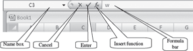
- Name Box—It displays the cell reference, or column and row location, of the active cell in the workbook window.
17.5 THE OFFICE BUTTON
The functionality of the Office button in MS-Excel is almost similar to the functionality provided in the MS– Word software. For example, New will open a blank document in MS–Word and a blank Workbook in MS-Excel.
The Office Button is used to perform file management operations on the file (i.e. the workbook). It contains commands that allow the user to create a new workbook, open an existing workbook, save a workbook, print a workbook etc. The Office button contains nine commands (Figure 17.6), namely, New, Open, Save, Save As, Print, Prepare, Send, Publish, and Close. The working of these commands is almost similar to their working in MS–Word. Here, we will discuss them briefly.
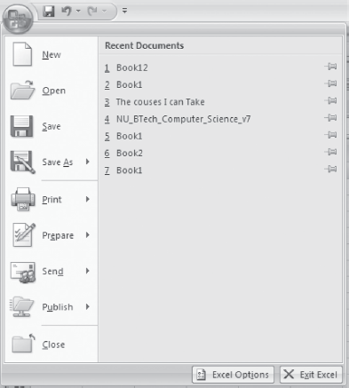
Figure 17.6 The office button commands
Table 17.1 briefly describes the different commands available in the Office Button.
| Office Button Commands | Description |
|---|---|
| New | Create a new blank workbook. |
| Open | Open an already existing workbook. |
| Save | Save a workbook for which a file name and location has already been specified. |
| Save As | Use when you save a workbook for the first time or to a differents location, or at the same location with a different name or with a new type of work book. Here, you specify the filename for the workbook, the location where the workbook is to be stored, and the save type of the workbook. You can also save the workbook as a Excel Workbook, Excel Binary Workbook, Excel 97–2003 workbook etc. (Figure 17.7). |
| Print, Quick Print, and Print Preview the workbook. You can set properties like print quality, paper type etc. and print the active sheet or the entire workbook. Preview to see how the workbook will look after printing. | |
| Prepare | Prepare the workbook for distribution. View workbook properties, encrypt document, restrict permissions etc. |
| Send | Send a copy of the workbook to e-mail or to Internet Fax. |
| Publish | Distribute the workbook to other people—Save for Excel services, share the workbook by saving it to a document management server, or create a new site for the workbook. (Figure 17.8). |
| Close | Close an open workbook. |
Table 17.1 Office button commands description
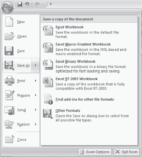
Figure 17.7 Save as option
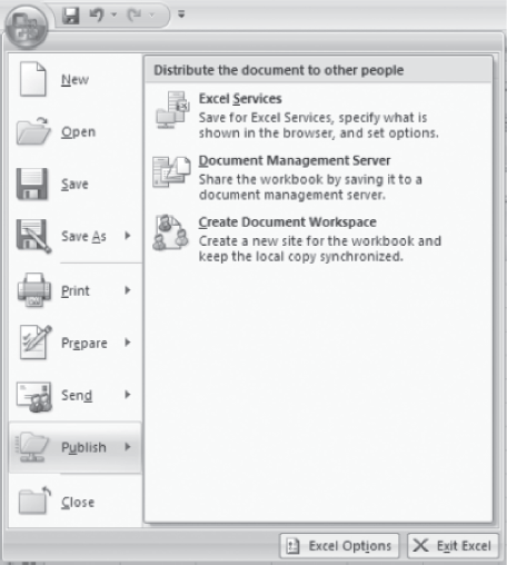
Figure 17.8 Publish option
The following describes briefly some of the common operations that are performed using the commands of the Office Button.
- Create a New Workbook: <> <New>. A new window opens up. <Blank Workbook> <Create>. There are templates available on the left panel for creating a workbook of a specific type (e.g. billing statement, sales report).
- Saving a Workbook for the First Time: <> <Save As>. Excel will display a dialog box. In the field next to File name, type a name with which you want to save the workbook. Navigate in the top portion of the dialog box to the folder where you want to save the workbook (choose the appropriate directory where you want to save the file. You can use
 to go up in the directory, Use
  to create a new folder). Once you have saved your workbook for the first time, you can save further revisions by selecting the <> <Save>, or by clicking on the Save button in the Quick Access Toolbar.
 - Saving a Workbook Under a Different Name: Open the workbook by selecting the <> <Open>. Next, <> <Save As>. A dialog box will appear. Navigate to the folder where you want to save the workbook and type in a new name for the workbook. Select the Save button. You now have two copies of the workbook, one with the original name, another with a new name.
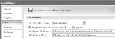
- Crash Protection: <> <Save As> <Tools><Save Options>. Select the boxes for Save Auto Recover Information every <enter the number of minutes>. Reset the Minutes from 10 to 1. MS-Excel would be able to recover a file one minute old.
- To Print: <> <Print>. Make settings like number of copies you want to print. (Figure 17.9). From the Print dialog box you can make further settings like—Print What, where you select what you want to print:
- Active worksheet
- Entire workbook; or
- The selection
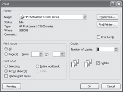
Figure 17.9 Print dialog box
Quick Tips—How to Learn MS-Excel
When working with MS-Excel, all you need to know is the following:
- What a command does?
- When you want to perform a particular action, which command to use?
- How to use a command?
Let’s see how we can go about learning MS-Excel.
What a command does—When your keep the mouse pointer over a command or icon, the function of the command or icon gets displayed in a text box. So it can be known what that command does, by moving the mouse over the command.
Which command to use—
- To search for a command, first see which tab might have the command. For example, if any formatting is to be done, click the Home Tab; to insert anything click the Insert tab; to use Formula, click the Formulas tab.
- It is possible to find the required group and command, most of the time. The commands that have similar uses are grouped together in the same group in Excel 2007.
Once the command is known, then we need to know how to use the command.
- For most of the commands, first place the cursor in the worksheet at the position where the action is to happen, or, select the object on which you want the action to happen (for example formatting commands). Next, click on the command. The command gets executed.
- In some commands, there are a set of steps to use the command.
17.6 THE RIBBON
Like the other programs in the Office 2007 suite, MS-Excel 2007 has a ribbon. The Ribbon of MS-Excel has the Office button and eight Tabs, namely, Home, Insert, Page Layout, Formulas, Data, Review, View, and Add–Ins. Each tab further consists of the groups, and the groups contain icons. Icons are pictorial representations for a command. The tabs in the Ribbon are self-explanatory; for example, if you want to do a page setup for the worksheet, click on the Page Layout tab. The groups and icons related to Page Layout are displayed. Select the appropriate command. The different tabs in MS-Excel and the groups within them are as follows:
- Home: Clipboard, Font, Alignment, Number, Styles, Cells, Editing
- Insert: Tables, Illustrations, Charts, Links, Text
- Page Layout: Themes, Page Setup, Scale to Fit, Sheet Options, Arrange
- Formulas: Function Library, Defined Names, Formula Auditing, Calculation
- Data: Get External Data, Connections, Sort & Filter, Data Tools, Outline
- Review: Proofing, Comments, Changes
- View: Workbook Views, Show/Hide, Zoom, Window, Macros
The Add-Ins Tab contains supplementory functionality that adds custom commands and specialized features to MS-Excel.
| Selecting a command | |
|---|---|
| Ways to select a command | Using a command |
| Click on a Tab + Click on a Icon |
Click on any of the Tabs like Home, Insert etc. From the displayed icons, click on the icon you want to use. |
| Shortcut key Ctrl + letter |
Some commands have shortcuts where you can press the Ctrl key and a certain letter. Some commonly used shortcuts are— |
| • Paste: CTRL + V • Copy: CTRL + C • Undo: CTRL + Z • New document: CTRL + N • Open document: CTRL + O • Print document: CTRL + P |
|
The commands in the Ribbon have various symbols associated with them, as shown in Figure 17.10. These symbols are interpreted as follows:
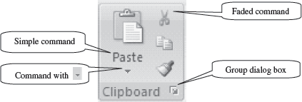
Figure 17.10 Command symbols
- Simple Command—The command start executing when it is clicked.
- Command Followed by Arrow—Clicking on the arrow displays more options for the command.
- Faded Command—A faded command means that it is not available currently.
- Group Dialog Box—Clicking on this symbol displays the dialog box for the group.
The following sub-sections describe the different tabs in detail.
Working with MS-Excel 2007
- Live Preview applies temporary formatting on the selected data or text when the mouse moves over any of the formatting buttons. This allows the preview of, how the text will appear with this formatting. The temporary formatting is removed if the mouse pointer is moved away from the button.
- Mini Toolbar is a floating toolbar that pops up whenever a test is selected or right-clicked. It provides easy access to the most commonly used formatting commands such as Bold, Italics, Font, Font size, Font color.
- File Format for the documents created in Excel 2007 is xlsx. (For earlier versions it was .xls)
17.6.1 The Home Tab
The Home Tab contains commands that are frequently used in an Excel worksheet. It contains commands for formatting of text and numbers, and text alignment. The Home Tab is also used for editing the content of sheet like sort and filter, find and select, and, to perform clipboard operations such as cut, copy, and paste on the sheet. Figure 17.11 shows the Home Tab.
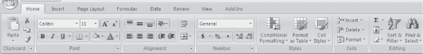
Figure 17.11 The home tab
There are seven groups within this tab, namely, Clipboard, Font, Alignment, Number, Styles, Cells, and Editing.
- The Clipboard group contains the cut, copy, and paste commands. The Format Painter is also present here. The Clipboard commands are used in the same manner as you use the MS–Word Clipboard commands.
- Font group commands allow change of the Font—font face, style, size, and color. These options can be changed before or after typing the text. The text whose font needs to be changed should be selected and then with the font commands in the Ribbon, or by menu obtained after right-click, the font can be changed.
- Alignment group is used to change alignment of the text in the cells—vertical and horizontal alignment, indentation, wrap the text, shrink it to fit within the cell, and merge multiple cells.
- Number group contains commands for number formatting e.g. Number, Date, accounting, decimals, comma style and percentage.
- The Styles group can be used to specify conditional formatting by defining formatting rules, convert a range of cells into a table by selecting a pre-defined Table Style, or, format a selected cell by selecting one of the built-in formatting styles.
- Cells allow the user to insert, delete or format the cells, and also whole columns, rows or sheets. Formatting includes renaming, hiding or protecting.
- Editing group contains commands to display the sum of selected cells, copy a pattern, clear the data, formats, and comments from a cell, sort and filter, or find and select specific contents within the workbook.
Table 17.2 gives the commands in the different groups (in left to right order) of the Home Tab along with a brief explanation.
| Home Tab Groups | Description |
|---|---|
| Clipboard |  • Cut removes the selected item from the sheet and pastes it onto a new place, where the cursor is pointing by using the paste command. • Copy copies the selected item and puts it on the Clipboard. • Format painter copies formatting from one place and applies it to another (To apply same formatting to many places, double-click the format painter button.) |
| Font |  • Increase font size, Decrease font size. • Bold, Italics, Underline • Apply borders to the currently selected cell. • Change the font color • Click on the arrow in dialog box. • Color the background of the selected cells. the bottom right corner of font to see the Format Cells |
| Alignment |  • Change the text orientation within a cell for placing a label above a column. • Left align, center, or right align for horizontal alignment in a cell. • increase or decrease, the amount of indentation within a cell. •.Wrap the text to make all content within a cell visible by displaying it on multiple lines. • Merge or unmerge the selected cells together and center the content of the cell. • Click on the arrow in the bottom right corner of Alignment to see the Format Cells dialog box. |
| Number | 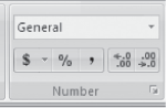 • Format the cell content to convert a number to a currency, percent, or decimal. Quick stvles allows to choose a visual style for the shape or line • Increase or decrease the number of zeroes after the decimal (degree of precision) • Click on the arrow in the bottom right corner of Number to see the Format Cells dialog box |
| Styles | 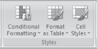 • Format a range of cells and convert the range to a table by selecting a pre-defined table style. • Cell Styles are pre-defined styles available to quickly format a cell |
| Cells |  • Delete rows or columns • Format the cell—change row height or column width, change visibility, protect or hide cells |
| Editing | 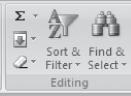 • Fills a pattern into one or more adjacent cells • Clear deletes everything from a cell, or remove formatting, contents, or comments • Sort & Filter arranges data for easy analysis (data can be sorted in ascending or descending order, or filter out specific values) • Find & Select (or replace) specific text, formatting or type of information within the workbook |
Table 17.2 Home tab commands description
Here, we describe briefly some of the operations that are performed using the commands of the Home Tab.
- Move Text: Select and highlight the section you want to move <Home><Clipboard>
 . Move the cursor to the place you would like the text to be inserted <Home><Clipboard>
 .
. - Copy Text: Select and highlight the section you want to copy <Home><Clipboard>
 . Move the cursor to the place you want the copied text to be inserted <Home><Clipboard>.
 - Find and Replace: This is used to find a text and then replace it with a new one. This option is use ful if you want to find a text at multiple places in the worksheet and replace all of them with a new one.
17.6.2 The Insert Tab
The Insert Tab contains commands for inserting objects of different kinds in a sheet. The commands in this tab are used to add illustrations, tables, links, text, and charts in a worksheet. Figure 17.12 shows the Insert Tab.

Figure 17.12 The insert tab
There are five groups within this tab, namely, Tables, Illustrations, Charts, Links, and Text.
- Tables are used to define a range of cells as a table for easy filtering and sorting, and create a pivot table or pivot chart to arrange and summarize data.
- Illustrations group allows insertion of pictures, clip art, shapes, and smart art.
- The Charts group helps to display data in a visual manner. It is used to insert different types of charts such as bar charts and pie charts.
- The Links group is used to insert a hyperlink to a place in the same workbook or an external one.
- The Text group contains commands to insert a Text Box, Word Art, Symbol, Digital Signature and Header And Footer.
Some of the Tabs appear only when you use them; like Picture Tools tab, Drawing Tools Tab, Table Tools Tab, and Chart Tools Tab
Table 17.3 gives the commands in the different groups of the Insert Tab along with a brief explanation.
| Insert Tab Groups | Description Groups |
|---|---|
| Tables | 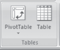 • Create a table to manage and analyze related data. Tables make it easy to sort, filter and format data within a sheet. When a table is drawn, a Table Tool Design Tab (Figure 17.14) open, Which allows you to select Table Style options, Table Styles, external table data etc. |
| Illustrations | 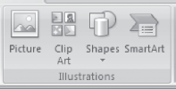 • Insert clipart into the document (sounds, movies, drawings) • Insert readymade shapes (lines, arrows, flowchart symbols etc.) into the document. A Drawing Tools Format Tab (Figure 17.16) opens. • Insert a smart art graphics. A Smart Art Tools Format tab opens. |
| Charts | 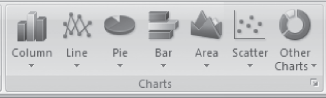 |
| Links |  |
| Text | 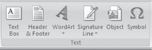 • Edit the header and footer to the sheet. You can insert the page number, date and time, sheet name, picture etc. A Header & Footer Tools Design Tab (Figure 17.18) opens up. • Insert decorative text in the document • Insert signature line that specifies the individual who must sign • Insert an embedded object. • Insert symbols that are part of the keyboard into the document. When you click on Symbol, a symbol table pops up. You can select the symbol you want to insert. |
Table 17.3 Insert tab commands description
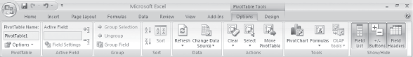
Figure 17.13 Pivot table tools options tab

Figure 17.14 Table tools design tab

Figure 17.15 Picture tools format tab
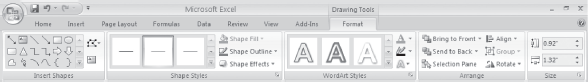
Figure 17.16 Drawing tools format tab
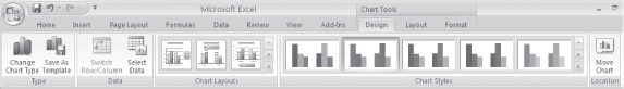
Figure 17.17 Chart tools design tab
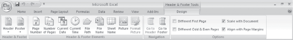
Figure 17.18 Header and footer tools design tab
When a command of the Insert tab is used, insertion takes place at the location where the cursor is present right now. So, before inserting the item, place the cursor at the location where the item is to be inserted. When you use the commands of the insert tab for insertion, you will see that most of the times, a dialog box will open which allows you to make specific settings, as per your requirement. Here, we do not discuss using the dialog boxes as they are self-explanatory, and are easy to use. Some of the operations using the Insert Tab commands are described below:
- To Create Headers and Footers—<Insert> <Text><Header & Footer>. Now you can edit the Header and Footer of your document. A Header and Footer tab is opened which allows you to add date and time, page number etc.
- Insert Hyperlink—<Insert> <Links> <Hyperlink>. To link to another location in the same document, click Place in This Document option under Link to; In the dialog box’s inner window, select a cell reference. To link to another document, click the Existing File or Web Page option. Navigate to the proper folder and select the file’s name. You can also add a link to a newly created document or an e-mail address.
- Insert Text—<Insert> <Text> <Text Box>. Click anywhere on the sheet where you want to insert the text box. Drag the corner points of the text box to change its size. Click within the box to type text. To format the text box, select the text box. <Drawing Tools> <Format>. Format the selected text box.
- Insert PivotTable—<Insert><Tables><PivotTable>. A Create Pivot Table dialog-box opens up. From the worksheet, select the table or range of cells to choose the data you want to analyze. (You must select the row headings). In the dialog box, select from whether you want to place the PivotTable in a new worksheet or an existing worksheet. Click <Ok>.

A PivotTable tools tab opens. On the right side of the sheet a PivotTable Field list is displayed. Select the fields to place in the PivotTable and drag the fields for column labels, row labels, report filter or values. A PivotTable is displayed. More settings can be done, using the PivotTable Options and Design tab. (Figure 17.19 shows the PivotTable created using the Names and Total marks of the students from a set of eight fields).

Figure 17.19 A pivot table example
17.6.3 The Page Layout Tab
The Page Layout Tab contains commands related to the layout and appearance of the pages in a document. It allows you to apply themes, change the page layout, and also provides options for viewing gridlines and headings. The Page Layout Tab is shown in Figure 17.20.
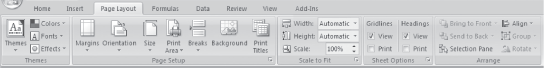
Figure 17.20 The page layout tab
There are five groups within this tab—Themes, Page Setup, Scale to Fit, Sheet Options, and Arrange.
- The Themes group contains commands to change the overall theme of current worksheet including fonts, colors, and fill effects.
- Page Setup is used to set the page margins, orientation, size, background, page breaks, print titles etc.
- Scale to Fit group allows specifying scaling of the page to force fit the document into a specific number of pages. It is possible to set the page width and height, stretch or shrink the printed output (scaling), and select the paper size and print quality.
- The Sheet Options group is used to switch sheet direction (right-to-left), view or print gridlines, and view or print worksheet headings (letters at the top of the sheet and numbers to the left of the sheet).
- The Arrange group is used to arrange, align or group the shapes and objects in the worksheet.
Table 17.4 gives the commands in the different groups of Page Layout Tab along with a brief explanation.
| Page Layout Tab Group | Description |
|---|---|
| Themes | 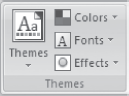 |
| Page Setup | 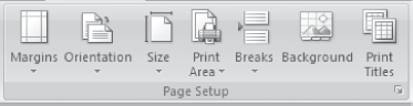 • Select orientation between portrait and landscape. • Choose a paper size for the current section. • Mark a specific area of the sheet for printing. • Specify when a new page will begin in a printed copy. • Choose an image as a background of the sheet. • Specify the rows and columns to repeat on each page. |
| Scale to Fit | 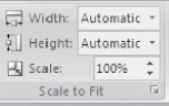 • Scale the printed output to a percentage of its actual size |
| Sheet Options | 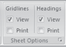 |
| Arrange | 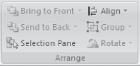 • Align the edges of multiple selected • Group objects together so that they can be treated like a single group. • Rotate or flip the selected object horizontally, vertically, by 90° etc. |
Table 17.4 Page layout commands description
- Specify page margins—<Page Layout><Page Setup><Margins> Change either top, bottom, left, or right margins by clicking in the appropriate text boxes or on the arrows next to the numbers in Custom margins.
17.6.4 The Formulas Tab
The Formulas Tab allows the user to define equations in order to perform calculations on values in the worksheet. The Formulas Tab is shown in Figure 17.21.
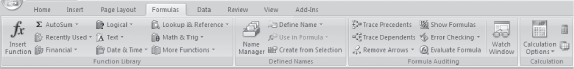
Figure 17.21 The formulas tab
There are four groups within this tab, namely, Function Library, Defined Names, Formula Auditing, and Calculation.
- The Function Library contains a library of functions (e.g. mathematical, logical, trigonometric, and math) that can be used to calculate or manipulate data.
- Defined Names allows the user to define names to be used to refer to specific formulas, and then allows searching for those names.
- Formula Auditing group includes commands to display formulas rather than results in a cell window, check for common formula errors, or trace precedents or dependents in cells that are referenced within a formula.
- Calculation allows user to specify calculation options for formulas—manual, automatic etc.
Table 17.5 gives the commands in the different groups of the Formulas Tab along with a brief explanation.
| Formulas Tab Group | Description |
|---|---|
| Function Library |  • Display the sum of the selected cells after the selected cells. • Browse and select from a list of logical functions like AND, IF. • Browse and select from a list of lookup and reference functions like ADDRESS, LOOKUP. • Browse and select from a list of recently used functions. • Browse and select from a list of text functions like LEN, Replace. • Browse and select from a list of math and trigonometric functions like ABS, FLOOR. • Browse and select from a list of financial functions like DISC, DB. • Browse and select from a list of date and time functions like DATE, HOUR. • Browse and select from a list of statistical, engineering and cube functions like AVERAGE, COMPLEX. |
| Defined Names | 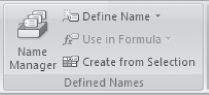 • Name cells so that can be referred in the formulas by that name. • Choose a name from this workbook and use it in the current formula. • Automatically generate names from the selected cells. |
| Formula Auditing | 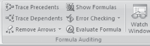 • Display the formula in the resulting cell instead of the resultant value. • Trace Dependents—Show arrows to indicate what cells are affected by the currently selected cell. • Check for common errors that occur in formulas. • Remove the arrows drawn by Trace Precedents and Trace Dependents. • Launch the Evaluate Formula dialog box to debug the formula. • Monitor the value of certain cells as changes are made to the sheet. |
| Calculation |  • Calculate the entire workbook now. • Calculate the current sheet now. |
Table 17.5 Formulas tab commands description
The formula addressing is briefly described below.
- Formula addressing—The formula can have relative addressing, absolute addressing, and mixed addressing.
- Relative address—To repeat the same formula for many different cells, use the copy and paste command. The cell locations in the formula are pasted relative to the position we copy them from. In the original cell we wrote =SUM(B5:C5); when we copy this formula in the cell below, we see that the formula becomes =SUM(B6:C6), i.e. the function will look at the two cells to its left.

- Absolute address—To keep a certain position that is not relative to the new cell location, use absolute positioning. For this, insert a $ before the column letter or a $ before the row number (or both). The $ sign locks the cell location to a fixed position. For example, =SUM($B$5:$C$5) will copy the same formula to every location we copy.
- Mixed address—A mix of relative and absoluter addresses is used to keep some part relative and some absolute. For example, =SUM(B$5:C$5) has the column address relative and the row address absolute.
- Relative address—To repeat the same formula for many different cells, use the copy and paste command. The cell locations in the formula are pasted relative to the position we copy them from. In the original cell we wrote =SUM(B5:C5); when we copy this formula in the cell below, we see that the formula becomes =SUM(B6:C6), i.e. the function will look at the two cells to its left.
17.6.5 The Data Tab
The Data Tab contains the commands related to the retrieval and layout of data that is displayed on a worksheet. The Data Tab is shown in Figure 17.22.
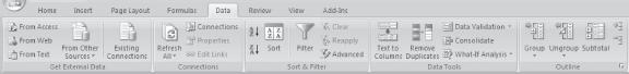
Figure 17.22 The data tab
There are five groups within this tab, namely, Get External Data, Connections, Sort & Filter, Data Tools, and Outline.
- The Get External Data group allows you to import data into Excel from external sources, such as an Access database, a Web page, a text file, etc.
- Connections include commands needed to create and edit links to external data or objects that are stored in a workbook or a connection file.
- The Sort & Filter group contains commands associated with sorting and filtering the data within a worksheet.
- Data Tools contains commands to remove duplicates, data validation, what if analysis, etc.
- Outline enables the user to group and ungroup a range of cells, and apply subtotals in a given column based on values of another column.
The commands in the different groups of the Data Tab along with a brief explanation are shown in Table 17.6.
| Data Tab Group | Description |
|---|---|
| Get External Data |  • Connect to an external data source by selecting from a list of commonly used sources. |
| Connections |  • Display all data connections for the workbook. • Specify how cells connected to a data source will update, what contents from the source will be displayed etc. • View all of the other files this spreadsheet is linked to, so that a link can be updated or removed. |
| Sort & Filter |  • Launch the Sort dialog box to sort based on several criteria all at once. • Enable filtering of the selected cells. • Clear the filter and the sort state for the current range of data. • Reapply the filter and sort in the current range. • Specify complex criteria to limit which records are included in the result set of a query. |
| Data Tools |  • Delete duplicate rows from the sheet. • Prevent invalid data from being entered into a cell. • Combine values from multiple ranges into one new range. • Try out various values for the formulas in the sheet. |
| Outline |  • Ungroup the range of cells that were previously grouped. • Total several rows of related data together by automatically inserting subtotals and totals for the selected cells. • Show or hide a group of cells. |
Table 17.6 Data tab commands description
17.6.6 The Review Tab
The Review Tab contains commands for review and revision of an existing document. The Review Tab is shown in Figure 17.23.

Figure 17.23 The review tab
There are three groups within this tab, namely Proofing, Comments, and changes.
- The Proofing group has commands required for the proofing of the document. It allows the spelling and grammar check, translate or check synonyms in the thesaurus, translate text into a different language, and search through reference materials such as dictionary or encyclopedia.
- Comments group contains commands to insert comments and move back and forth among the comments.
- The Changes group contains command to protect the workbook by restricting its access. It allows the user to specify how a workbook can be edited or shared with others, and allows the user to keep track of the changes made to it.
The commands in the different groups of the Review Tab along with a brief explanation are shown in Table 17.7.
| Review Tab Group | Description |
|---|---|
| Proofing |  • Open Research Task Pane and search through research material. • Thesaurus suggests word similar in meaning to the selected word. • Translate the selected text into a different language. |
| Comments |  • Edit or Delete the selected comment. • Navigate to the previous or the next comment. • Show or hide comment attached to the selected cell. • Display all the comments in the sheet. • Show or hide any ink annotations on the sheet. |
| Changes |  • Allow multiple people to work in a workbook at the same time. • Share the workbook and protect it with a password at the same time. • Allow specific people to edit ranges of cells in a protected workbook or sheet. • Track all changes made to the document including insertions, deletions and formatting changes. |
Table 17.7 Review tab commands description
17.6.7 The View Tab
The View tab has commands that affects how the document appears on the screen. The View Tab is shown in Figure 17.24.

Figure 17.24 The view tab
There are five groups within this tab, namely, Workbook Views, Show/Hide, Zoom, Window, and Macros.
- The Workbook Views group has commands to view the document in different modes like normal, page break view etc. You can also create your own custom views or switch to full screen view.
- The Show/Hide group contains commands to show or hide the ruler, gridlines, message bar, formula bar, or worksheet headings.
- Zoom is used to view the document in smaller or larger sizes. You can zoom in and out with different options.
- Window group contains commands to create new windows, arrange all open windows and switch between them, freeze panes so that they continue to appear on the screen while scrolling, and save a workspace.
- The Macros group is used to create or view a macro. Macros allow you to define a sequence of actions to perform on a document or multiple documents that can be executed again and again simply by running the macro.
The commands in the different groups of View Tab along with a brief explanation are shown in Table 17.8.
| View Tab Group | Description |
|---|---|
| Workbook Views | 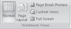 • Page layout allows viewing the document as it will appear in a Printed page. You can see where the pages begin and end and also to see the header and footer. • View a preview of where the pages will break when printed. • Save a set of display and print settings as custom view. • View the document in the full screen mode. |
| Show/Hide | 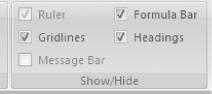 |
| Zoom |  • Zoom the worksheet so that the currently selected range of cells fills the entire window. |
| Window | 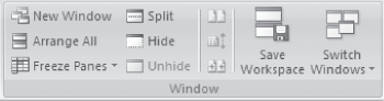 • Arrange all open sheets side-by-side on the screen. • Keep a portion of the screen visible while rest of the sheet scrolls. • Split the window into multiple re-sizable panes containing views of your worksheet. • Hide or unhide the current window. • View two worksheets side-by-side so that their contents can be compared. • Synchronize the scrolling of two documents so that they scroll together. • Reset the window position so that the documents share the space equally. • Save the current layout of the window as workspace so that they can be restored later on. • Switch to a different currently open window. |
| Macros |  |
Table 17.8 View tab commands description
17.6.8 The Help
The Help button ![]() is located on the right most side of the Tabs in the Ribbon. Click on this button to get help for using any command of the Excel. On clicking on the help button, a screen as shown in Figure 17.25 appears. You can browse the Help for the command you want. You can also perform operations such as, search for a command and view the Table of Contents.
is located on the right most side of the Tabs in the Ribbon. Click on this button to get help for using any command of the Excel. On clicking on the help button, a screen as shown in Figure 17.25 appears. You can browse the Help for the command you want. You can also perform operations such as, search for a command and view the Table of Contents.

Figure 17.25 Excel help
Many of the concepts that you use while working with MS–Office suite are common for MS–Word, MS–PowerPoint and MS-Excel. For example, open, close, save, cutting and pasting are performed the same way in MS-Excel as they are in MS–Word and MS–PowerPoint. The menus are also arranged in a similar layout. If you are not sure how to do something in Excel, then try it as you would do in MS–Word or MS–PowerPoint, and it may work.
17.7 SOLVED EXAMPLES
Example 1: The following table gives year-wise sale figures of five salesmen in Rs.

- Calculate total sale year-wise.
- Calculate the net sales made by each salesman.
- Calculate the commission for each salesman — If total sales is greater than Rs.1,00,000/-, then commission is 5% of total sale made by the salesman, else it is 2% of total sale.
- Calculate the maximum sale made by each salesman.
- Calculate the maximum sale made in each year.
- Draw a bar graph representing the sale made by each salesman.
- Draw a pie graph representing the sales made by salesmen in year 2004.
Solution 1:
- Open blank workbook. <New> <Create>
- Enter the headings of the table
- Double-click on the cell and type.
- If name is too long, use Text Wrap: <Home><Alignment><
 >
> - Use Text Orientation to change the direction of the text: <Home><Alignment><
 >
>
- Double-click on the cells and enter the data.
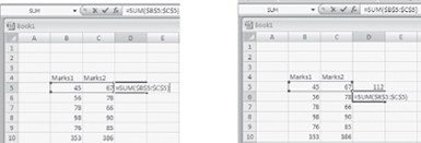
- Total Year-wise Sales: Since you want to find the total, the function SUM is used.
- If you already know that the SUM function is to be used, then type =SUM(. You will see that the format of the SUM function appears. Click on number1 in the format and select the cells for which you want to find the total. It will write =SUM(E10:E14. Close the brackets =SUM(E10:E14). This is the total sales of one year. Click on the cell in which you have found total and pull the plus sign to the other columns of the same row to get total year-wise sales of other years.
- If you do not know that the SUM function is to be used, then use the options <Formulas> <Function Library>. Look for the appropriate function.
- Net Sales for each Salesman: Same method as for Total Year-wise Sales.
- Commission: Enter the IF formula.
- Enter =IF(
- Then select the cells whose value is to be checked. It will become =IF(I10
- Write the condition. >100000,0.05*(
- Again select the cells. It will become =IF(I10>100000,0.05*(I10), 0.02*(
- Again select the cells, and put brackets.The final formula will look like=IF(I10>100000,0.05*(I10), 0.02*(I10))
- Maximum sale made by each salesman: Use MAX function: =MAX(E10:H10)
- Maximum sale made in each year: Use MAX function: =MAX(E10:E14)
- Select the cells and use <Home><Styles><Conditional Formatting> and <Home><Styles><Cell Styles> to give conditional formatting and style, respectively, to the cells.
- Bar graph: <Insert><Charts><Bar> A Chart Tools Tab appears
- Select <Chart Tools> <Design> Select a Chart Style or change the style using <Chart Tools><Type> <Change Chart Type>
- <Chart Tools><Data><Select Data>. A dialog box appears. Either enter the cell numbers, or you can select the cells from the worksheet for which you want to make a chart. When you select, a dotted border appears around the selected cells. Next, click <OK> in the dialog box.
- A chart appears. Now use the <Chart Tools> <Layout> <Labels> to label and decide the placement of your chart axes, legend, title etc.
- Use <Chart Tools> <Layout> <Current Selection> <Format Selection> to format the chart area like fill texture, gradient etc.
- Select <Chart Tools> <Design> Select a Chart Style or change the style using <Chart Tools><Type> <Change Chart Type>
- Pie graph: <Insert><Charts><Pie>. A Chart Tools Tab appears. Follow the same steps as in Bar graph.
Figure 17.26 and Figure 17.27 show the sales table and the graphs.
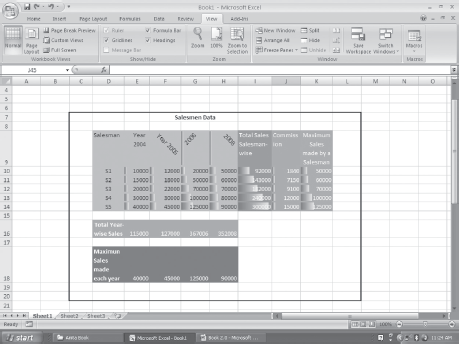
Figure 17.26 Sales table
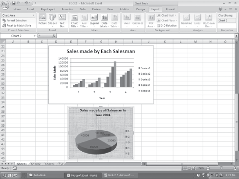
Figure 17.27 Bar graph and pie graph for the sales table example
Example 2: A school pays a monthly salary to its employees, which consists of basic salary, allowances, and deductions. The details of allowances and deductions are as follows:
- HRA is 30% of the Basic.
- DA is 20% of Basic.
- Conveyance Allowance is —
- Rs. 500/-, if Basic is less than or equal to Rs.10000/-
- Rs. 750/-, if Basic is greater than Rs.10000/- and less than Rs.20000/-
- Rs. 1000/-, if Basic is greater than Rs.20000/-
- Entertainment Allowance is —
- Rs 500/-, if Basic is less than or equal to Rs.10000/-
- Rs.1000/-, if Basic is greater than Rs.10000/-
- PF deduction is 6% of Basic.
- IT deduction is 15% of the Basic.
- Calculate the following:
- Gross Salary = Basic + HRA + DA + Conveyance + Entertainment
- Deduction = PF + IT
- Net Salary = Gross Salary — Deduction
Make a salary table and calculate the net salary of the employees.
Solution 2:
- Open blank workbook. <New> <Create>
- Enter the headings of the table
- Double-click on the cell and type.
- If name is too long, use Text Wrap: <Home><Alignment><
 >
> - Use Text Orientation to change the direction of the text: <Home><Alignment><
 >
>
- Double-click on the cells and enter the data.
- Select the cells and use <Home><Styles><CellStyles> to give style to the cells.
- For HRA enter the formula =0.03*D7
- For DA, enter the formula: =0.02*D7
- For Conveyance Allowance, write the formula: =IF(D7<=10000,500,IF(AND(D7>10000, D7<20000),750,1000))
- For Entertainment Allowance, enter the formula: =IF(D7<=10000,500,1000)
- For Gross Salary, enter formula: =SUM(D7:H7)
- For PF, enter formula: =0.06*D7
- For IT, enter formula: =0.15*D7
- For Net Deduction, enter formula: =SUM(J7:K7)
- For Net Salary, enter formula: =I7–L7
- Select the cells and use <Home><Styles><Conditional Formatting> and <Home><Styles><Cell Styles> to give different colors and style to the cells.
Figure 17.28 shows the salary table.
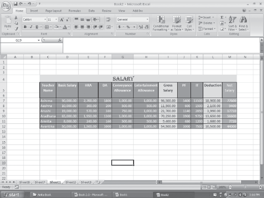
Figure 17.28 Salary example
Example 3: Make a sheet having the fields—S. No., Name, Physics Marks, Math Marks, Computer Sc. Marks, Total Marks, Percentage, and Grade. Fill the data for the S. No., Name, Physics Marks, Math Marks, and Computer Sc. Marks.
Calculate the following-
Find the Percentage of the student.
- Calculate Grade (A- > 90%, B- between 80%–90%, C- otherwise).
- Apply filter to display marks more than 80%.
- Enter the S. No. and get the Grade using VLOOKUP
- Sort all records on Name.
Solution 3:
- Open blank workbook. <New> <Create>
- Enter the headings of the table
- Double-click on the cell and type.
- If name too long, use Text Wrap: <Home><Alignment><
 >
> - Use Text Orientation to change direction of the text: <Home><Alignmentx><
 >
>
- Double-click on the cells and enter the data.
- To find the percentage, use the formula =SUM(I8)/300.
- To find Grade, use the formula =IF(J8>0.9,”A”,IF(J8>0.8,”B”,”C”)). Figure 17.29 shows the Student Table with percentage and grade calculated.
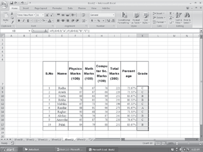
Figure 17.29 Student marks example
- Apply Filter:
- Select the column or columns on which you want to apply the filter. Here it is column Percentage.
- Click on <Data><Sort & Filter><Filter> You will see that an arrow like
 appears in that column.
 - Click on the arrow. A pop-up menu appears. Click on <Number Filters>. Select one of the displayed options. Here we select Greater Than… A Custom AutoFilter dialog box appears. Since we want all students having more than 80%, put .8 in the box on the right side. Click <OK>. Figure 17.30 shows filter applied to the Student Table.
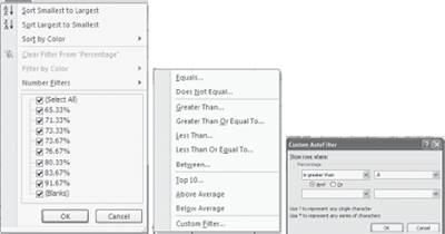
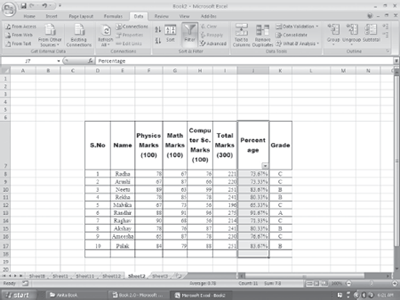
Figure 17.30 Student marks example with filter on percentage
- Using VLOOKUP: Use VLOOKUP formula, =VLOOKUP(D8,StudentTable,8)
- D8 is the cell number of the S.No field. So, the first argument is the field for which we want to find the result.
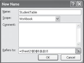
- Student Table is the name given to the whole table. You can specify the cell range or define a name for the Table. To specify cell range, simply select the complete table. To define a name for the table– Select the table. <Formulas><Defined Names> <Define Name>. A New Name dialog box appears. Write the Name with which you want to refer to the Table. Here we write Student– Table. Click <OK>. In the VLOOKUP formula, the second argument is the table name.
- The third argument is the column number from where you want the result. Here we want the Grade, which is the 8th column in the Table.
- So, use the formula =VLOOKUP(D8,StudentTable,8). Figure 17.31 shows VLOOPUP reference in the Student table.
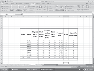
Figure 17.31 Student marks example with VLOOKUP reference
- To sort the table on the field Name: Select the column on the basis of which you want to sort. Click <Data><Sort & Filter> <Sort>.
- If only one column of the table is selected, you get a Sort Warning. Click on <Expand the Selection> and <Sort>. You get the sorted table.
- If you select multiple columns you get the Sort dialog box. Here you can specify the levels of sorting also (for example, level 1—sort on name, level 2—sort on total marks etc.). Click <OK>. You get the sorted table. Figure 17.32 shows the Student table after sorting.
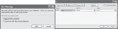
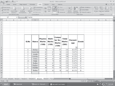
Figure 17.32 Student marks example with sort on name
Exercises:
- Design a mark-sheet for a student as follows:
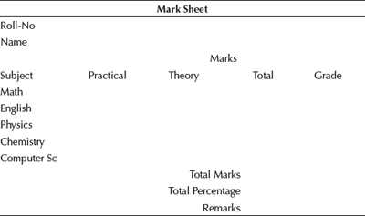
- Calculate the total marks for each subject. Calculate the grade (A-90% or more, B - 80%-less than 90%, C-70% - less than 80%, D-60% - less than 70%, E-otherwise)
- Calculate the total marks of all subjects and the total percentage. Depending on the total percentage write the following in remarks
- Excellent-90% or more
- Very Good-80%-less than 90%,
- Good-70%-less than 80%,
- Fair-60%-less than 70%,
- Poor-less than 60%
- Use cell style to show colored cells
- Use thick outline border
- Use Font size, color and alignment for the text
- Design the Time Table given to you at the start of the Semester, without grid lines.
- Prepare a schedule of your exams.
- Prepare the rate list of the Mother Dairy Fruit and Vegetable Vendor:
- Sort the Table in decreasing order of rate list.
- Find the total of all the rates.
- While printing the table hide the gridlines.
- Check the spelling and grammar in an existing document. Use the “Replace” option in Find and Replace to replace each instance of some word.
- Create a 7-column, 6-row table to create a calendar for the current month.
- Enter the names of the days of the week in the first row of the table.
- Centre the day names horizontally and vertically.
- Change the font and font size as desired.
- Insert a row at the top of the table. Merge the cells in the row and enter the current month and year using a large font size. Shade the row.
- Enter and right-align the dates for the month in the appropriate cells of the table.
- Change the outside border to a more decorative border. Identify two important dates in the calendar, and shade them.
- In a new workbook, create the worksheet. Name the worksheet as Furniture Details. Enter the data shown in the table below:
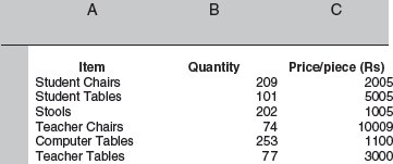
- Calculate the total amount for each item (Quantity*Price/Piece) and also the total amount for all items.
- Apply suitable formatting to currency entries (Rs.) and numbers.
- Adjust the column widths where needed. Insert blank rows between column labels and data.
- Use alignments, fonts, borders, and colors to format the “Furniture Details” worksheet. For example, put a border around the title, change the color of column headings to red, and center all the entries in Column B.
- Create a header that includes your name, and a footer that includes current date. Change page orientation to Landscape.
- Preview and print the worksheet.
- Use the Furniture Table in Question 11 to do the following:
- Prepare a bar chart for the data. Place the chart as an object in the worksheet.
- Print the entire worksheet with the chart.
- Print the entire worksheet without the chart.
- Change the bar chart to an exploded pie chart. Add a title to the pie chart.
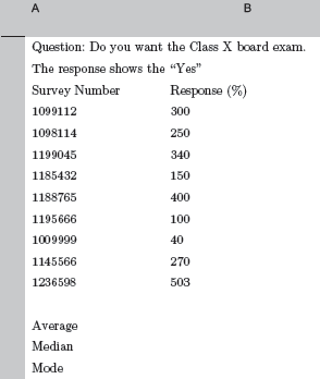
- Create a worksheet as shown below:
- Calculate the average, mode, and median.
- Draw a bar graph.
- Color all the responses more than 20% in a different color. Count these responses.
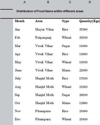
- Create a worksheet as shown below:
- Sort the data in the “Type” column. Filter the areas where “Rice” is supplied.
- Use PivotTables in the this worksheet that uses the SUM function in the quantity. Change the SUM function to AVERAGE or COUNT.
- Add/modify one or two new records to the data, and then reset the range for the PivotTable.
- Open two documents and view them together.
- Design a worksheet using the following functions—MODE, STDDEV, VARIANCE, MEDIAN, SIN, COS, TAN, COUNT, MAX, MIN, ABS, MOD, SUM, SUMIF, POWER
- Design a worksheet as follows:

- Enter data in the worksheet. (at least 15 records).
- Calculate the total charges for each member. If a member does not avail of a facility, the corresponding charge for that activity should be zero.
- Generate a separate report of the members who are not availing any of the facility.
- Draw a chart for each facility showing its percentage of use. (For example if 5 out of 15 people are not using swimming facility, the chart should show—swimming facility as 66.6%used,and the rest unused)
- Use the appropriate function to list the facility that is being most often used.
- Use appropriate function to find the members using the club facility the most.(Hint: maximum non-zero entries)
- Print the reports.
The above questions can be made specific by including one or more of the following options:
- Create and name range data to simplify use.
- Use Names and Labels in functions.
- Use Decision–Making functions such as SUMIF to calculate data based on the evaluation ?of criteria in another data range.
- Use Nested functions such as IF, AND, and OR to analyze data based on multiple conditions.
- Run and record a macro.
- Save macros in a Personal Workbook, the current workbook, or in a new workbook.
- Open multiple workbooks simultaneously.
- Copy and paste between workbooks.
- Use copy and Paste Special.
- Link data in multiple workbooks.
- Write linking formulas.
- Consolidate data based on its position in a worksheet.
- Consolidate data based on data categories.
- Outline worksheets to display or print various levels of worksheet detail.
- Use Pivot Tables to summarize and analyze large banks of data.
- Modify and expand a pivot table.
- Insert and rename sheet tabs.
- Change column width and row height.
- Use formula with Relative and Absolute cell addresses.
- Analyze formula syntax.
- Use Auto Sum, Auto Calculate, and AutoFill.
- Apply number formats to support worksheet data.
- Align cell entries, apply text formats, and apply cell borders for visual clarity.
- Clear cell contents, comments, and formatting.
- Undo and redo multiple actions.
- Spell check a worksheet.
- Insert and delete rows.
- Copy data to a predefined range.
- Use comments in a worksheet.
- Use Dates in functions.
- Use Conditional Formatting.
- Create Lists.
- Sort on one column or multiple columns.
- Filter list data to select specific date—Filter with custom criteria, Use Advanced Filters, Remove a filter, Use AutoFilter.
- Use Subtotals.
- Use the Chart Wizard to embed a chart on an Excel worksheet—bar, column, line, and pie charts.
- Create a chart on a separate chart sheet.
- Read series formulas that underlie charts.
- Size or move a chart or a chart object.
- Change chart types.
- Format charts to improve their appearance.
- Print charts with the corresponding worksheet data.
- Protect a Worksheet.
- Create a Template.
- Use a Template to Create a Workbook (Hint: <Office button> <New>).
- Import data into Excel.
- Export data from Excel into a text file.