4.3 Conditional Control
When more than one flow option exists in the control flow, it is called a conditional control flow. Whenever a certain condition is met, its respective flow option is followed. A condition is an expression defined using relational and Boolean operators that evaluate to either true or false. The list and interpretation of the supported relation operators is presented in Table 4-1.
|
Relational operator |
Meaning |
|
== |
Equal to |
|
!= |
Not equal to |
|
< |
Less than |
|
> |
Greater than |
|
<= |
Less than or equal to |
|
>= |
Greater than or equal to |
An example of the use of relational operators to form relational expressions is shown in Example 4-1.
irb(main):001:0> 5 == 5
=> true
irb(main):002:0> 5 == 6
=> false
irb(main):003:0> 5 <= 5
=> true
irb(main):004:0> 5 != 5
=> false
To create complex expressions, simple relational expressions are
combined by using Boolean operators. Two Boolean variable operators
available in Ruby are and and or. The operator and evaluates to true only if both operands are
true. In contrast, the operator or
evaluates to true if either or both operands are true. To ensure the
precedence you desire, a good programming practice is to use parentheses.
A truth table is presented in Table 4-2.
|
A |
B | A and B | A or B |
| (alternate forms) | A&&B | A||B | |
|
True |
True | True | True |
|
True |
False | False | True |
|
False |
True | False | True |
|
False |
False | False | False |
Recall the negation operator (!)
that appears in the not equal to relational operator. This operator is a
simple negation and works on any true or false expressions or
conditionals, as shown in Example 4-2. Sometimes the negation
operator ! is denoted by the word
not. In fact, the fifth example in the
figure, regardless of the Boolean values you set for first and second, will always evaluate to true. This is
called a tautology.
irb(main):001:0> !false
=> true
irb(main):002:0> !(true or false)
=> false
irb(main):003:0> first=true
=> true
irb(main):004:0> second=false
=> false
irb(main):005:0> (first and second) or !(first and second)
=> true
Control Flow
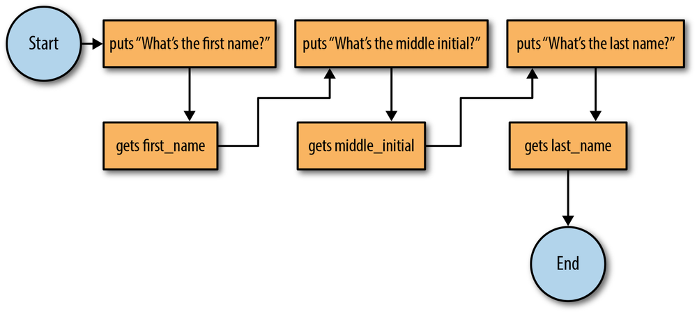
Control flow is logic flow in the context of a program. Just as algorithms start somewhere and show an order of steps until the end of the algorithm, so does a program. Programs have a starting instruction, and then instructions are executed in a specific order, and eventually the program ends. We use a flowchart to illustrate control flow. Figure 4-3 revisits the names example to illustrate control flow with flowcharts. Note that the start and endpoints of the algorithms are indicated by circular shapes (circles or ovals depending simply on the length of text contained).
This type of flow is known as one-directional control flow. Programs are not limited to one-directional control flow. In this chapter, we discuss programming constructs that allow us to change program control flow. Understanding this control flow is essential to being able to create and test (debug) an implementation of an algorithm.