5. consolidate the results

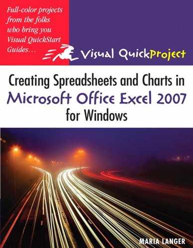
We now have three worksheets full of budget and actual information. Our next step is to consolidate this information into one summary worksheet for the quarter. We’ll do that with Excel’s consolidation feature.

prepare the sheet

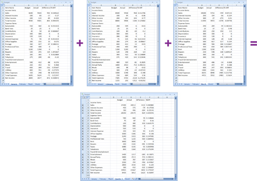
The consolidated information will go on its own sheet. We can prepare the sheet by activating it, renaming it, and activating the first cell of the consolidation range.

1. Click the sheet tab for Sheet2 to activate it.

2. Follow the instructions on page 24 to name the sheet tab Quarter 1.

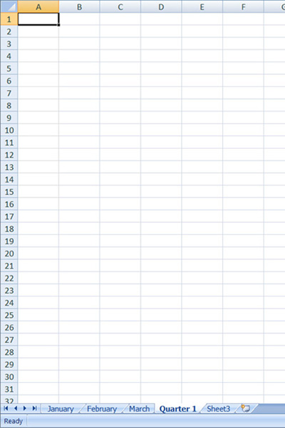
3. Activate cell A1.

consolidate

Excel’s consolidation feature uses the Consolidate dialog to collect your consolidation settings, including the worksheet ranges you want to include in the consolidation and the type of consolidation you want to perform.

1. Click the Data tab on the Ribbon.

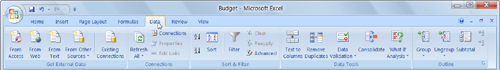
2. Click the Consolidate button in the Data Tools group.

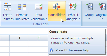
The Consolidate dialog appears.

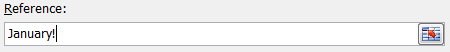
5. Click the January sheet tab so that sheet becomes active behind the dialog. January! appears in the Reference box.

6. Position the mouse pointer on cell A1.

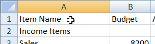
7. Press the mouse button and drag down and to the right to select from cell A1 to cell D28. As you drag, the Consolidate dialog collapses so you can see what you’re doing and a selection marquee appears around the cells you drag over.

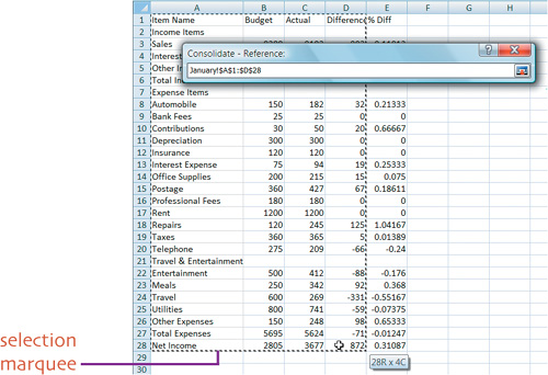
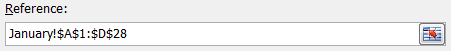
8. Release the mouse button. The range you selected appears in the Reference box.

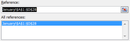
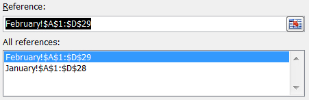
9. Click Add. The reference is copied to the All references box.

10. Click the February sheet tab to activate that sheet. February!$A$1:$D$28 appears in the Reference box and a selection marquee in the worksheet behind the dialog indicates that range of cells.

11. Position the mouse pointer on cell A1.

12. Press the mouse button and drag down and to the right to select from cell A1 to cell D29. As you drag, the Consolidate dialog collapses.

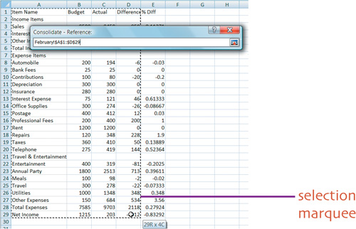
13. Release the mouse button. The range you selected appears in the Reference box.

14. Click Add. The reference is copied to the All references box.

15. Click the March sheet tab so that sheet becomes active. March!$A$1:$D$29 appears in the Reference box and a selection marquee in the worksheet indicates that range of cells.

16. Position the mouse pointer on cell A1.

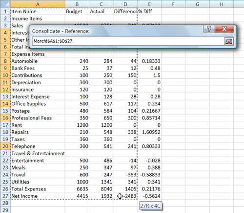
17. Press the mouse button and drag down and to the right to select from cell A1 to cell D27. As you drag, the Consolidate dialog collapses.

18. Release the mouse button. The range you selected appears in the Reference box.

19. Click Add. The reference moves to the All references box.

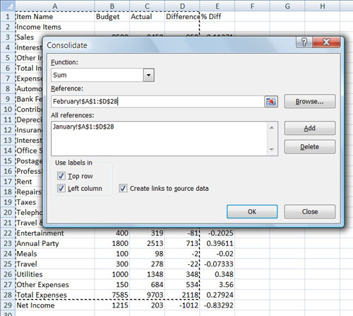
At this point, the Consolidate dialog should look like this.

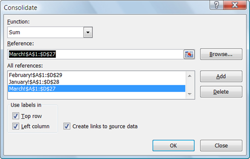
20. Click OK.

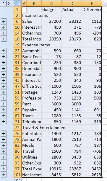
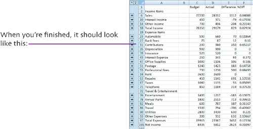
Excel creates the consolidation and displays it in the Quarter 1 worksheet.

check the consolidation

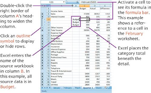
When you consolidate multiple worksheets as instructed here, you create a new worksheet with “3-D” references to the source worksheets. Because Excel has to display contents from all of the source cells, it automatically displays the consolidation as an outline with the outline collapsed so only the total for each category appears.

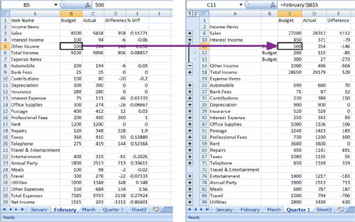
If one of the source worksheets changes, the consolidation automatically changes.

calculate percent diff

When we created our consolidation, we omitted the percent difference calculation on the source worksheets. The reason: Our consolidation used the SUM function to add values in the source worksheets. Adding the percentages would result in incorrect values for the consolidated percent differences. As a result, we need to recreate the percent difference formula in the consolidation worksheet and copy it to the appropriate cells.

1. Click the sheet tab for the Quarter 1 worksheet to activate that sheet.

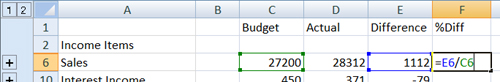
2. Enter % Diff in cell F1 and press Enter.

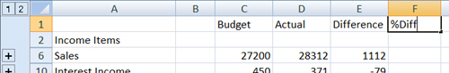
3. Enter the formula =E6/C6 in cell F6. You can either type it in or follow the procedure on page 34 to enter the formula by typing and clicking. (If you do click, be sure to click in the correct cells!) Don’t forget to press Enter to complete the formula.

4. Use techniques on pages 39–42 to copy the formula to cells F10 to F18, F23 to F71, and F76 to F101.

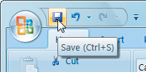
Have you been saving your work?

Now is a good time to click the Save button on the Quick Access toolbar to save your work up to this point.

extra bits

consolidate pp. 59–62

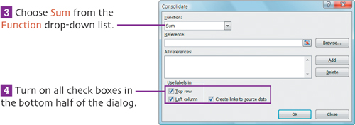
• Because each worksheet in the consolidation has a slightly different organization—remember, we added a row in one and deleted a row in another—you must turn on the Left column check box to properly consolidate. Doing so tells Excel to sum values based on category name (the row label) rather than row position.

calculate percent diff p. 64

• If you use the fill handle to copy the formula in cell F6 to other cells, Excel automatically copies the formula to cells in hidden rows you drag over. This doesn’t really matter, though, since we’re only interested in the consolidated numbers and will keep the hidden rows hidden.

shortcut keys for this chapter