
Chapter 14
Graphs
In This Chapter
Graphs are among the most versatile structures used in computer programming. They appear in all kinds of problems that are generally quite different from those we’ve dealt with thus far in this book. If you’re dealing with general kinds of data storage problems such as records in a database, you probably don’t need a graph, but for some problems—and they tend to be interesting ones—a graph is indispensable.
Our discussion of graphs is divided into two chapters. In this chapter we cover the algorithms associated with unweighted graphs, show some problems that these graphs can represent, and present a visualization tool to explore them. In the next chapter we look at the more complicated algorithms associated with weighted graphs.
Introduction to Graphs
Graphs are data structures rather like trees. In a mathematical sense, a tree is a particular kind of graph. In computer programming, however, graphs are used in different ways than trees.
The data structures examined previously in this book have an architecture intertwined with the algorithms used on them. For example, a binary tree is structured the way it is because that “shape” makes it easy to search for data and insert new data. The links between nodes in a tree represent quick ways to get from parent to child.
Graphs, on the other hand, often have a shape dictated by a physical or abstract problem. For example, nodes in a graph may represent cities, whereas edges (links) may represent airline flight routes or roads or railways between the cities. Another more abstract example is a graph representing the individual tasks necessary to complete a project. In the graph, nodes may represent tasks, whereas directed edges (with an arrow at one end) indicate which task must be completed before another. In both cases, the shape of the graph arises from the specific real-world situation.
If graphs represent real-world things, what can they be used for? Well, the ones that describe transportation links can be used to find all the possible ways of getting from one place to another. If you’re only interested in the shortest path (or maybe the longest), there are algorithms that use graphs to find that path. When the graph represents communication between people, you can find clusters of people that form communities or organizations. Similarly, communication graphs can be used to find people or groups that are isolated from one another.
Before going further, we must mention that, when discussing graphs, nodes are traditionally called vertices (the singular is vertex). The links between vertices are called edges. The reason is probably that the nomenclature for graphs is older than that for trees, having arisen in mathematics centuries ago.
Definitions
Figure 14-1 shows a simplified map of the major freeways in the vicinity of Seattle, Washington. Next to the map is a graph that models these freeways.
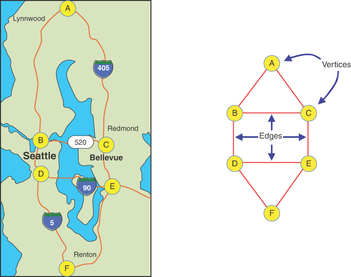
FIGURE 14-1 Roadmap and a corresponding graph
In the graph, circles represent freeway interchanges, and straight lines connecting the circles represent freeway segments. The circles are vertices, and the lines are edges. The vertices are usually labeled in some way—often, as shown here, with letters of the alphabet. Each edge connects and is bounded by the two vertices at its ends.
The graph doesn’t reflect the exact geographical positions shown on the map; it shows only the relationships of the vertices and the edges—that is, which edges are connected to which vertex. It doesn’t concern itself with physical distances or directions (even though the figure shows them in roughly the same orientation as the map). The primary information provided by the graph is the connectedness (or lack of it) of one intersection to another, not the actual routes.
Adjacency and Neighbors
Two vertices are said to be adjacent to one another if they are connected by a single edge. Thus, in Figure 14-1, vertices C and E are adjacent, but vertices C and F are not. The vertices adjacent to a given vertex are said to be its neighbors. For example, the neighbors of vertex D are B, E, and F.
Paths
A path is a sequence of edges. The graph in Figure 14-1 has a path from vertex A to vertex F that passes through vertices B and D. By convention, we call this path ABDF. There can be more than one path between two vertices; another path from A to F is ACEF. Because this graph came from a road network, you can easily see the correspondence of real-world routes to paths in the graph.
Connected Graphs
A graph is said to be connected if there is at least one path from every vertex to every other vertex, as in the graph in Figure 14-1. If “You can’t get there from here” (as a rural farmer might tell city slickers who stop to ask for directions), the graph is not connected. For example, the road networks of North America are not connected to those of Japan. A nonconnected graph consists of several connected components. In Figure 14-2, two graphs with the same group of vertices are shown. In the graph on the left, all five vertices are connected, forming a single connected component. The graph on the right has two connected components: B-D and A-C-E.
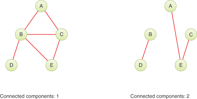
FIGURE 14-2 Connected and nonconnected graphs
Note that an edge always links two vertices in a graph. It would be incorrect to eliminate, for instance, vertex D in the right-hand graph of Figure 14-2 and leave a “dangling” edge connected to B.
For simplicity, the algorithms we discuss in this chapter are written to apply to connected graphs or to one connected component of a nonconnected graph. If appropriate, small modifications usually enable them to work with nonconnected graphs as well.
Directed and Weighted Graphs
Figure 14-1 and Figure 14-2 show undirected graphs. That means that the edges don’t have a direction; you can go either way on them. Thus, you can go from vertex A to vertex B, or from vertex B to vertex A, with equal ease. Undirected graphs model rivers and roads appropriately because you can usually go either way on them (at least, slow-flowing rivers). Sometimes undirected graphs are called bidirectional graphs.
Graphs are often used to model situations in which you can go in only one direction along an edge—from A to B but not from B to A, as on a one-way street, the northbound or southbound lanes of a freeway, or downstream on a river with waterfalls and rapids. Such a graph is said to be directed. The allowed direction is typically shown with an arrowhead at the end of the edge. A valid path in a directed graph is a sequence of edges where the end vertex of edge J is the start vertex of edge J + 1.
In some graphs, edges are given a numeric weight. The weight is used to model something such as the physical distance between two vertices, or the time it takes to get from one vertex to another, or how much it costs to travel from vertex to vertex (on airline routes, for example). Such graphs are called weighted graphs. We explore them in the next chapter.
In this chapter we start the discussion on simple undirected, unweighted graphs; later we explore directed, unweighted graphs. We have by no means covered all the definitions and descriptions that apply to graphs; we introduce more as we go along.
The First Uses of Graphs
One of the first mathematicians to work with graphs was Leonhard Euler in the early eighteenth century. He solved a famous problem dealing with the bridges in the town of Konigsberg, on the Baltic coast. This town on a river included an island and seven bridges, as shown in Figure 14-3.
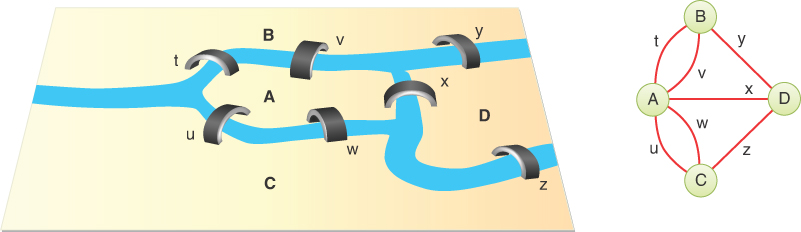
FIGURE 14-3 The bridges of Königsberg
The problem, much discussed by the townsfolk, was to find a way to walk across all seven bridges without recrossing any of them. We don’t recount Euler’s solution to the problem; it turns out that there is no such path. The key to his solution, however, was to represent the problem as a graph, with land areas as vertices and bridges as edges, as shown at the right of Figure 14-3. This is perhaps the first example of a graph being used to represent a problem in the real world.
Note that in the graph of the Königsberg bridges, multiple bridges connect the different land areas. For example, the island, A, connects to the lower bank of the river, C, by bridges u and w. The graph shows multiple edges, and the edges are labeled to distinguish them. The term for a graph that allows multiple edges to connect a single pair of vertices is a multigraph. In this the case, the edge labels aren’t weights—just ways to distinguish the possible paths between vertices A and C.
Representing a Graph in a Program
It’s all very well to think about graphs in the abstract, as Euler and other mathematicians did, but you want to represent graphs using a computer. What sort of software structures are appropriate to model graphs? Let’s look at vertices first and then at edges.
Vertices
In an abstract graph program, you could simply number the vertices 0 to N–1 (where N is the number of vertices). You wouldn’t need any sort of variable to hold the vertices because their usefulness would result from their relationships with other vertices.
In most situations, however, a vertex represents some real-world object, and the object must be described using data items. If a vertex represents a city in an airline route simulation, for example, it may need to store the name of the city, the name of the airport, its altitude, its location, runway orientations, and other such information. Thus, it’s usually convenient to represent a vertex by an object of a vertex class. Our example programs store only a name string (like A), used as a label for identifying the vertex. Listing 14-1 shows how the basic Vertex class might look.
LISTING 14-1 The Basic Vertex Class
class Vertex(object):        # A vertex in a graph
   def __init__(self, name): # Constructor: stores a vertex name
      self.name = name       # Store the name

   def __str__(self):        # Summarize vertex in a string
      return '<Vertex {}>'.format(self.name)
Note that the name attribute is declared public here. The reason is that you can allow it to be manipulated by the caller during various operations without affecting the graph containing it.
Vertex objects can be placed in an array and referred to using their index number. The vertices might also be placed in a list or some other data structure. The unique vertex index or the object itself can identify this vertex within a graph.
For vertices with coordinates like latitude and longitude, storing them in a quadtree may make sense, as described in Chapter 12, “Spatial Data Structures.” It is important to have them in some structure that preserves their unique identifiers so that even if the caller changes the name or other attribute, the vertex can be retrieved. If you use a quadtree, you could not allow the coordinates of the vertex to change without changing its placement in the quadtree. For graphs with simply labeled vertices, an array is fine for storage if the vertex always stays at its original index.
Whatever structure is used for vertices, this storage is for convenience only. It has no relevance to how they are connected by edges. For edges, you need another mechanism.
Edges
In Chapter 8, “Binary Trees,” you saw that a computer program can represent trees in several ways. Mostly that chapter examined trees in which each node contained references to its children, but you also learned that an array could be used, with a node’s position in the array indicating its relationship to other nodes. Chapter 13, “Heaps,” described arrays used to represent a particular kind of tree called a heap.
A graph, however, doesn’t usually have the same kind of fixed organization as a tree. In a binary tree, each node has a maximum of two children, but each vertex in a graph may be connected to an arbitrary number of other vertices. For example, in Figure 14-2, the left-hand graph’s vertex B is connected to four other vertices, whereas D is connected to only one.
To model this sort of free-form organization, a different approach to representing edges is preferable to that used for trees. Several methods are commonly used for graphs. We examine two (although some might call it three): the adjacency matrix and the adjacency list. Remember that one vertex is said to be adjacent to another if they’re connected by a single edge, not a path through several edges.
The Adjacency Matrix
An adjacency matrix can be represented as a two-dimensional array in which the elements indicate whether an edge is present between two vertices. If a graph has N vertices, the adjacency matrix is an N×N array. Table 14-1 shows an example of an adjacency matrix for the left-hand graph of Figure 14-2, repeated here.
Table 14-1 Adjacency Matrix
A | B | C | D | E | |
A | 0 | 1 | 1 | 0 | 0 |
B | 1 | 0 | 1 | 1 | 1 |
C | 1 | 1 | 0 | 0 | 1 |
D | 0 | 1 | 0 | 0 | 0 |
E | 0 | 1 | 1 | 0 | 0 |
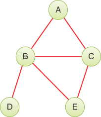
The vertex labels are used as headings for both rows and columns. An edge between two vertices is indicated by a 1; the absence of an edge is a 0. (You could also use Boolean True/False values.) As you can see, vertex B is adjacent to all four other vertices; A is adjacent to B and C; C is adjacent to A, B, and E; D is adjacent only to B; and E is adjacent to B and C. In this example, the “connection” of a vertex to itself is indicated by 0, so the diagonal from upper left to lower right, A-A to E-E, which is called the identity diagonal and shaded gray, is all 0s. The entries on the identity diagonal don’t convey any real information, so you can equally well put 1s along it, if that’s more convenient to a program. (A kind of graph called a pseudograph allows edges that go from a vertex to itself. Such graphs can use the diagonal of the adjacency matrix to represent the presence or absence of such edges.)
Note that the triangular-shaped part of the matrix above the identity diagonal is a mirror image of the part below; both triangles contain the same information. This redundancy is a bit inefficient, but there’s no simple way to create a triangular array in most computer languages, so it’s simpler to accept the redundancy. Consequently, when you add an edge to the graph, you make two entries in the adjacency matrix rather than one.
Note, in this chapter, we focus on unweighted graphs, and the edges don’t need separate labels like in the bridges of Königsberg. Graphs that allow multiple edges between a single pair of vertices are called multigraphs. They can be quite useful as in the case of the bridges of Königsberg but are beyond the scope of this text.
Using Hash Tables for the Adjacency Matrix
One way to improve storage efficiency is to keep the matrix as a hash table rather than a two-dimensional array. To do this, the hash table must accept keys with two parts—one for each vertex. That’s straightforward, as discussed in Chapter 11, “Hash Tables.” The individual characters in a string or the indices in a tuple can be hashed using different weights in the hashing function to produce a single hash index.
To represent an edge using a hash table adjacency matrix, you make an entry at a particular pair of vertices. For example, to add an edge between vertices 2 and 7, you would insert a value for the key (2, 7). Using the data structures from Chapter 11, you could write
adjacencyMatrix = HashTable()
adjacencyMatrix.insert((2, 7), True)
After the edges are placed in the matrix, programs can determine whether two edges are adjacent by using the hash table’s search() method. For example, to see whether two vertices are adjacent, you would evaluate adjacencyMatrix.search((4, 12)). If no entry had been made for (4, 12), the search would return None, which Python treats as False in a Boolean context. If an entry had been made for that key, its True value would be returned.
With either hash tables or two-dimensional arrays, you can avoid the duplicate storage of the two triangular halves of the matrix by always using the smaller vertex index in the first position. In other words, to check if vertex 19 is adjacent to vertex 8 by a bidirectional edge, you would check the matrix at (8, 19) instead of (19, 8). Reordering the vertex indices would be necessary for all operations on the matrix—insertion, deletion, and searching. That adds a little extra time to each of those operations. The alternative of adding time to the insertion and deletion operations by using both orderings and updating both matrix cells is usually preferable when searching will be much more frequent than inserting and deleting. It also is better for directional graphs, as you see later.
Hash tables have an extra benefit over two-dimensional arrays when there are few edges. If a graph has, for example, a thousand vertices and two thousand edges, the two-dimensional array needs storage for a million cells while the hash table needs only enough for the two thousand edges (so perhaps four thousand cells). The difference becomes significant for large graphs because the memory needed for two-dimensional arrays is O(N2), where N is the number of vertices, limiting what can be kept in the computer’s memory.
On the other hand, two-dimensional arrays are easier to decompose into rows and columns. Many graph algorithms were developed to take advantage of the capability to access rows and columns quickly. The choice of representation depends on what operations need to be done quickly on the graph.
The Adjacency List
The other common way to represent edges is with a list. The list in adjacency list refers to a linked list of the kind examined in Chapter 5, “Linked Lists.” In actuality, an adjacency list is an array of lists, or sometimes a list of lists, or sometimes a list stored in each Vertex. Each individual list contains references to the adjacent vertices of that vertex. Table 14-2 shows the adjacency lists for the left-hand graph of Figure 14-2, repeated here.
Table 14-2 Adjacency Lists
Vertex | Adjacent Vertices List |
|---|---|
A | B→C |
B | A→C→D→E |
C | A→B→E |
D | B |
E | B→C |
In this table, the → symbol indicates a link in a linked list. Each link in the list is a vertex. Here, the vertices are arranged in alphabetical order in each list, although that’s not strictly necessary. More likely, the order of the vertices would depend on the order the edges were added to the graph.
Don’t confuse the contents of adjacency lists with paths. The adjacency list shows which vertices are adjacent to—one edge away from—a given vertex, not paths from vertex to vertex.
In the next chapter we discuss when to use one of the adjacency matrices as opposed to an adjacency list. The Visualization tool shown in this chapter shows the adjacency matrix approach, but in many cases, the list approach is more efficient.
Adding Vertices and Edges to a Graph
To add a vertex to a graph, you make a new Vertex object, insert it into a vertex array or list, and grow the adjacency structure, as we discuss shortly. In a real-world program, a vertex might contain many data elements, but for simplicity of the program examples, you can assume that it contains only a single attribute, its name. (The Visualization tool also associates different colors with the vertices in addition to their names to indicate the different data they reference.) Thus, the creation of a vertex looks something like this:
vertices.append(Vertex('F'))This command inserts a vertex object named F at the end of the Python array called vertices.
How you add an edge to a graph depends on whether you’re using an adjacency matrix or adjacency lists to represent the graph. Let’s say that you’re using an adjacency matrix and want to add an edge between vertices 1 and 3. These numbers correspond to the array indices in vertices where the vertices are stored.
When the adjacency matrix was created, it would have a particular size. If adding a new vertex means it needs an extra row and column, the array will need to grow. When the adjacency matrix, adjMat, is first created, it is filled it with 0s or perhaps a Boolean False. When it grows, all the new cells must be filled with that same value. Adjacency matrices represented as hash tables do not require growing when new vertices are added. They grow when edges are added as new keys as described in Chapter 11, “Hash Tables.”
Two-Dimensional Arrays and Python
To insert the edge between vertices 1 and 3 in two-dimensional arrays in Java or C++, you could write
adjMat[1][3] = 1;
adjMat[3][1] = 1;
The core Python language supports only one-dimensional arrays, although extensions like NumPy provide multidimensional arrays. You can store an array in the cell of another array to approximate multidimensional arrays. For example, you can create an array of vertices plus an adjacency matrix, and insert an edge with code like the following:
vertices = []                  # A list of vertices
vertices.append(Vertex('A'))
vertices.append(Vertex('B'))
vertices.append(Vertex('C'))
vertices.append(Vertex('D'))

adjMat = [ [False for v in range(len(vertices))]
           for _ in range(len(vertices)) ]
adjMat[1][3] = True
adjMat[3][1] = True
To create the adjacency matrix, we’ve used nested list comprehensions that create an outer array filled with arrays. The inner comprehension, [False for v in range(len(vertices))], creates a list/array of four cells filled with the value False. The outer comprehension repeats the inner creation four times to create four cells filled with lists/arrays. The result of the last two assignment statements leaves adjMat holding
[[False, False, False, False],
 [False, False, False, True],
 [False, False, False, False],
 [False, True,  False, False]]
The True values show up in the rows and columns indexed by (1, 3) and (3, 1). Note that Python’s capability to expand a list/array using the multiplication operator doesn’t work correctly here. If you try
badMat = [ [False] * len(vertices) ] * len(vertices)
badMat[1][3] = True
the resulting badMat array contains
[[False, False, False, True],
 [False, False, False, True],
 [False, False, False, True],
 [False, False, False, True]]
That’s not what you want, but why did it come out that way? The reason is that the multiplication operator fills the cells of the expanded list with the exact same value. The inner multiply creates a four-cell array of False values. The outer multiply does the same kind of expansion, and every cell is filled with a reference to the same inner four-cell array. Because the same inner array is shared among all the cells of the outer array, assigning True to cell 3 in one row affects all the rows.
Storing Edges in Adjacency Lists
Returning to the concept of using adjacency lists, they have a similar nested list/array structure, but with a significant difference. Instead of each row having the same length, they are variable-length lists of vertex indices. For example,
adjList = [ [] for v in range(len(vertices)) ]
adjList[1].append(3)
adjList[3].append(1)
produces an array containing
[[], [3], [], [1]]
The cells of this array contain lists of vertex indices. Cell 0 has the (empty) list of vertices for vertex 0, and so on. The complete adjacency list shows that vertices 0 and 2 have no edges, whereas vertices 1 and 3 share an edge.
Note that the multiplication operator also fails to work for adjacency lists too. For example,
badList = [[]] * len(vertices)
badList[1].append(3)
produces
[[3], [3], [3], [3]]
The list comprehension method effectively executes a loop to create separate elements for its output array; that’s how it builds separate lists on each iteration.
The Graph Class
Let’s make this discussion more concrete with a Python Graph class that constructs a vertex list and an adjacency matrix and contains methods for adding vertices and edges. Listing 14-2 shows the code.
This implementation makes use of Python’s list type to manage the list of vertices and the dict type to store the adjacency matrix. These two structures behave like the Stack and HashTable classes you saw in earlier chapters, but with some different syntax. The constructor for the Graph creates an empty list called _vertices and an empty dict called _adjMat. You saw hash tables used to store a grid of cells in Chapter 12, “Spatial Data Structures.” In case you skipped that, we describe the use of Python’s dict type as a dictionary (hash table) in more detail here.
The pair of curly braces, {}, in the constructor creates an empty hash table that can accept most Python data structures as a key. For this graph, we use tuples of vertex indices, like (2, 7), as the keys to the adjacency matrix. When we need to store a 1 in the adjacency matrix for a particular tuple, we could write
self._adjMat[(2, 7)] = 1
The square brackets after _adjMat surround the key to the hash table. That tells Python that it should hash the key inside to find where to place the value in the hash table. Later we can retrieve the value from the hash table using the same syntax.
You can also use the slightly simpler syntax
self._adjMat[2, 7] = 1
to do the same thing. To programmers familiar with other languages, this syntax might look like a multidimensional array reference, but it is not. The comma in the expression within the brackets tells Python to construct a tuple. In this case, it constructs the tuple (2, 7) and uses that as the key for the hash table. The hashing function uses all the tuple elements in calculating the hash table index. This means that the value gets stored in a unique location for the key (2, 7). In a two-dimensional array, the cell at row 2, column 7 would be addressed, but in the hash table, some location in its one-dimensional array is used. To the calling program, it doesn’t matter which one, as long as that exact same cell is found when it references (2, 7) in the hash table later.
LISTING 14-2 The Basic Graph Class
class Graph(object):         # A graph containing vertices and edges
   def __init__(self):       # Constructor
      self._vertices = []    # A list/array of vertices
      self._adjMat = {}      # A hash table mapping vertex pairs to 1

   def nVertices(self):      # Get the number of graph vertices, i.e.
      return len(self._vertices) # the length of the vertices list

   def nEdges(self):         # Get the number of graph edges by
      return len(self._adjMat) // 2 # dividing the # of keys by 2

   def addVertex(self, vertex): # Add a new vertex to the graph
      self._vertices.append(vertex) # Place at end of vertex list

   def validIndex(self, n):  # Check that n is a valid vertex index
      if n < 0 or self.nVertices() <= n: # If it lies outside the
         raise IndexError    # valid range, raise an exception
      return True            # Otherwise it's valid

   def getVertex(self, n):   # Get the nth vertex in the graph
      if self.validIndex(n): # Check that n is a valid vertex index
         return self._vertices[n] # and return nth vertex

   def addEdge(self, A, B):  # Add an edge between two vertices A & B
      self.validIndex(A)     # Check that vertex A is valid
      self.validIndex(B)     # Check that vertex B is valid
      if A == B:             # If vertices are the same
         raise ValueError    # raise exception
      self._adjMat[A, B] = 1 # Add edge in one direction and
      self._adjMat[B, A] = 1 # the reverse direction

   def hasEdge(self, A, B):  # Check for edge between vertices A & B
      self.validIndex(A)     # Check that vertex A is valid
      self.validIndex(B)     # Check that vertex B is valid
      return self._adjMat.get( # Look in adjacency matrix hash table
         (A, B), False)      # Return either the edge count or False
Note that the Python syntax for addressing one-dimensional arrays and hash tables is identical. When Python sees var[2], it looks at the type of the var variable to determine what to do next. If var is a list, then the expression in the brackets should be an integer index to one of its array cells. If var is a dict, then the contents of the brackets hold a key to be hashed. The tuples of vertex numbers such as (2, 7) are treated as a single hash key.
Moving on to the first method defined in the Graph class of Listing 14-2, you find that nVertices() makes use of Python’s len() function to get the length of the list/array holding the vertices. A freshly constructed Graph has an empty _vertices list, so the length is zero.
The second method, nEdges(), is similar but uses the length of the hash table, _adjMat, in its calculation. Python uses the number of keys that have been stored in the hash table as its length. Because we plan to store vertex pairs along with their mirror image—for example (2, 7) and (7, 2)—as separate keys for each edge, the total number of edges is half the number of keys.
The third method, addVertex(), adds a vertex to the graph by using Python’s built-in append() method on the _vertices list. This is just like pushing an element on a stack (assuming the top of the stack is the end of the list). We left out a check in this method that the vertex argument is one of the Vertex objects as defined in Listing 14-1, but that would be good to include.
Next, the program introduces a simple test for a valid vertex index, validIndex(). Because callers specify vertices by their index, they could specify indices outside the range of those already added to the graph. This predicate—a function with a Boolean result—checks whether the index lies outside of the range [0, nVertices), raising the IndexError exception if it does. This is the same exception that Python uses for invalid array indices.
The getVertex() method gets a vertex from the graph based on an index, n. After the index is validated, the vertex object can be retrieved from the array.
The addEdge() method takes two vertex indices, A and B, as parameters. To create the edge, it first verifies that both A and B are valid vertex indices. Without these checks, the Graph could become internally inconsistent. It also checks whether A and B are the same index. That would create an edge from a vertex to itself. This simple Graph class doesn’t allow the creation of pseudographs. Finally, the method updates the adjacency matrix to create the edge. It uses both orders of the vertices because the edge is bidirectional.
We now have a basic Graph object that can expand to accept any number of vertices and edges. The next important method is one that tests whether an edge exists between two vertices. The hasEdge() method takes two vertex indices, A and B, as parameters. They are checked for validity like before. With valid indices, the adjacency matrix can be checked to see whether an edge was defined. You might expect to use the same Python syntax, _adjMat[A, B], to test for that edge. That, however, causes a problem if the edge does not exist. Python hash tables raise a KeyError exception when asked to access a key that has not been previously inserted.
There are a couple of ways to address missing keys in the adjacency matrix. One is to catch the KeyError exception that could occur when accessing _adjMat[A, B]. The other is to use Python’s get() method for hash tables, which is what this implementation does. The get() method takes the key as the first parameter plus a second one for the value to return if the key is not in the hash table. We pass the tuple, (A, B), for the key. The default value is set to False so that hasEdge() returns that when the edge does not exist. If the edge does exist, the call to get() will return 1, the value that was inserted by addEdge(), which is interpreted as True in Boolean contexts.
Another way to implement the hasEdge(A, B) check would be to return the value of this expression (A, B) in self._adjMat. Python uses the in operator to test whether a key has been inserted in a hash table. Because we only ever set the values in _adjMat to 1, we could ignore the value and only check for the presence of the key. When edges are deleted, however, we could not simply set the value to 0 if we use the (A, B) in self._adjMat test; we would need to remove the key from the hash table.
Traversal and Search
One of the most fundamental operations to perform on a graph is finding which vertices can be reached from a specified vertex. This operation is used to find the connected components of a graph and underlies many more complex operations. When we look at a graph diagrams, it’s usually immediately obvious which vertices are connected, at least for simple graphs. To the computer, however, it must discover what vertices are connected by chaining together edges. Let’s look at some examples of discovering what’s connected.
Imagine that you are traveling to a foreign country by airplane or boat for a vacation. When there, you will be visiting the countryside by bicycle, and you want to know all the places you can go. Paved roads and some dirt roads would be good for the trip, but roads that are closed for repair or washed out with mud or floods are not worth traversing. The road conditions might be cataloged somewhere, but in some cases, you would have to go to a nearby location to find out whether the road was passable. Based on the road conditions, some towns could be reached, whereas others couldn’t. You still want to have the best vacation possible, so you would determine what places are accessible via bicycle and decide your route among them. You might have to remake the plan as you travel and learn more about road conditions in each area.
Other situations where you need to find all the vertices reachable from a specified vertex are in designing circuits and plumbing networks. Electronic circuits are composed of components like transistors that are connected by conductors such as wires or metal paths. In plumbing networks various components such as water heaters, faucets, drains, and gas stoves connect via pipes. Figure 14-4 shows small examples of an electronic circuit and a plumbing network. In both cases, many of the components are connected, and others are not. It’s critical to their function that the connections are complete. If not, hot water might not reach a particular faucet, or the signal from an antenna might not reach a decoder. Perhaps even more important, the disconnected vertices must remain that way—lest the power supply connect directly to a speaker or the gas supply connect to a faucet.
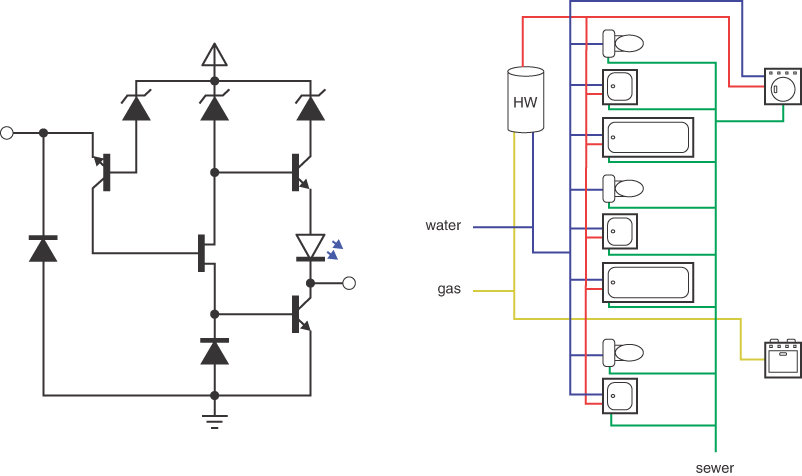
FIGURE 14-4 An electronic circuit and a plumbing network
In these kinds of networks, it’s important to find all the vertices connected to a given vertex. That defines the connected components of the graph. Each connected component must be realized in the form of electrical or plumbing connections. That’s often easy for you to see in diagrams like Figure 14-4, especially when the colors of the edges in the plumbing diagram clearly separate the kinds of pipes. It’s much less clear in the case of the road network for bicycling, especially when you must travel to an area to learn what’s connected and what’s not.
Assume that you’ve been given a graph that describes a network. Now you need an algorithm that provides a systematic way to start at a specified vertex and move along edges to other vertices in such a way that, when it’s done, you are guaranteed that it has visited every vertex that’s connected to the starting vertex. Here, as it did in Chapter 8, where we discussed binary trees, visit means to perform some operation on the vertex, such as displaying it, adding it to a collection, or updating one of its attributes.
There are two common approaches to traversing a graph: depth-first (DF) and breadth-first (BF). Both eventually reach all connected vertices but differ in the order they visit them. The depth-first traversal is implemented with a stack, whereas breadth-first is implemented with a queue. You can traverse all the connected vertices or perhaps stop when you find a particular vertex. When the goal is to stop at a particular vertex, the operation is called depth-first search (DFS) or breadth-first search (BFS) instead of traversal.
You saw in Chapter 8 that the different traversal orders of binary trees—pre-order, in-order, and post-order—had different properties and uses. The same is true of graphs. The choice of depth-first or breadth-first depends on the goal of the operation.
Depth-First
The depth-first traversal uses a stack to remember where it should go when it reaches a dead end (a vertex with no adjacent, unvisited vertices). We show an example here, encourage you to try similar examples with the Graph Visualization tool, and then finally show some code that carries out the traverse.
An Example
Let’s look at the idea behind the depth-first traversal in relation to the graph in Figure 14-5. The colored numbers and dashed arrows in this figure show the order in which the vertices are visited (which differ from the ID numbers used to identify vertices).
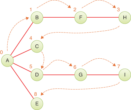
FIGURE 14-5 Depth-first traversal example
To carry out the depth-first traversal, you pick a starting point—in this case, vertex A. You then do three things: visit this vertex, push it onto a stack so that you can remember it, and mark it so that you won’t visit it again.
Next, you go to any vertex adjacent to A that hasn’t yet been visited. We’ll assume the vertices are selected in alphabetical order, so that brings up B. You visit B, mark it, and push it on the stack.
Now what? You’re at B, and you do the same thing as before: go to an adjacent vertex that hasn’t been visited. This leads you to F. We can call this process Rule 1.
Rule 1
If possible, visit an adjacent unvisited vertex, mark it, and push it on the stack.
Applying Rule 1 again leads you to H. At this point, however, you need to do something else because there are no unvisited vertices adjacent to H. Here’s where Rule 2 comes in.
Rule 2
If you can’t follow Rule 1, then, if possible, pop a vertex off the stack.
Following Rule 2, you pop H off the stack, which brings you back to F. F has no unvisited adjacent vertices, so you pop it. The same is true of vertex B. Now only A is left on the stack.
A, however, does have unvisited adjacent vertices, so you visit the next one, C. The visit to C shows that it is the end of the line again, so you pop it, and you’re back to A. You visit D, G, and I, and then pop them all when you reach the dead end at I. Now you’re back to A. You visit E, and again you’re back to A.
This time, however, A has no unvisited neighbors, so you pop it off the stack. Now there’s nothing left to pop, which brings up Rule 3.
Rule 3
If you can’t follow Rule 1 or Rule 2, you’re done.
Table 14-3 shows how the stack looks in the various stages of this process, as applied to Figure 14-5. The contents of the stack show the path you took from the starting vertex to get where you are (at the top of the stack). As you move away from the starting vertex, you push vertices as you go. As you move back toward the starting vertex, you pop them. The order in which you visit the vertices is ABFHCDGIE. Note that this is not a path, just a vertex list, because H is not adjacent to C, for example.
Table 14-3 Stack Contents During Depth-First Traversal
Event | Stack |
|---|---|
Visit A | A |
Visit B | AB |
Visit F | ABF |
Visit H | ABFH |
Pop H | ABF |
Pop F | AB |
Pop B | A |
Visit C | AC |
Pop C | A |
Visit D | AD |
Visit G | ADG |
Visit I | ADGI |
Pop I | ADG |
Pop G | AD |
Pop D | A |
Visit E | AE |
Pop E | A |
Pop A | |
Done |
You might say that the depth-first algorithm likes to get as far away from the starting point as quickly as possible and returns only when it reaches a dead end. If you use the term depth to mean the distance from the starting point, you can see where the name depth-first comes from.
An Analogy
One analogy to a depth-first search is solving a maze. The maze—perhaps one of the people-size ones made of hedges, popular in England, or corn stalks, popular in America—consists of narrow passages (think of edges) and intersections where passages meet (vertices).
Suppose that Minnie is lost in a maze. She knows there’s an exit and plans to traverse the maze systematically to find it. Fortunately, she has a ball of string and a marker pen. She starts at some intersection and goes down a randomly chosen passage, unreeling the string. At the next intersection, she goes down another randomly chosen passage, and so on, until finally she reaches a dead end.
At the dead end, she retraces her path, reeling in the string, until she reaches the previous intersection. Here she marks the path she’s been down, so she won’t take it again, and tries another path. When she’s marked all the paths leading from that intersection, she returns to the previous intersection and repeats the process.
The string represents the stack in depth-first: it “remembers” the path taken to reach a certain point. The pen represents marking vertices as visited. If Minnie didn’t have a pen, she could always choose, say, the leftmost passage to visit when arriving at an intersection. When returning along the string and coming back to an intersection, she would choose the next passage to the right to visit and continue to follow the string back if there were no more passages to the right. The critical thing is that Minnie needs to remember having visited an intersection/vertex so that she doesn’t just revisit them. The sense of left and right doesn’t exist in most graphs, and computers don’t use pens; they must use explicit marking.
The Graph Visualization Tool and Depth-First Traverse
You can try out the depth-first traversal with the Depth-First Traverse button in the Graph Visualization tool. Start the tool (as described in Appendix A, “Running the Visualizations”). At the beginning, there are no vertices or edges, just an empty shaded rectangle. You create vertices by double-clicking the desired location within the shaded box. The first vertex is automatically labeled A, the second one is B, and so on. They’re each given a different color.
To make an edge, drag the pointer from one vertex to another. Figure 14-6 shows part of the graph of Figure 14-5 as it looks while being created using the tool. The adjacency matrix appears in the lower-right corner. When the Visualization tool first starts, there are no vertices, and the matrix is empty. The matrix and the _vertices table in the upper right grow as you add vertices.
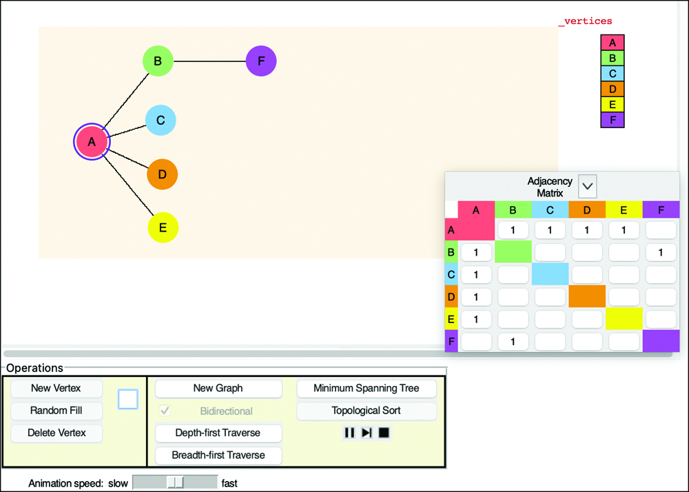
FIGURE 14-6 The Graph Visualization tool
You can edit the graph in many ways. Like the other Visualization tools, this one has buttons in the operations area that allow you to create and delete vertices by their label. Because the tool must find vertices by their label, all the names must be unique (and short enough to fit in the little circles and rectangles). When you add a vertex—say with the label V—the program will choose a random location for it within the shaded box and conveniently update the label in the text entry box to W in case you plan to add another. That allows you to click New Vertex N times to create N vertices with unique names. You can also put a number in the text entry box and select the Random Fill button to create that many more vertices.
If you want to rearrange the vertex positions, press and hold the Shift key while you click a vertex and drag it to its new position. The Visualization tool allows you to place the vertex only where it lies completely within the shaded box and does not overlap another vertex. If you want to get rid of a vertex or an edge, you can double-click it.
Another way to delete edges is by clicking the box corresponding to that edge in the adjacency matrix table. Because edges are either present or absent in this kind of graph, each click toggles the edge on or off. You can collapse the adjacency matrix by pressing the ![]() button and restore it with the
button and restore it with the ![]() button. That capability is especially useful for large graphs.
button. That capability is especially useful for large graphs.
To run the depth-first traversal algorithm, select a starting vertex by clicking it and then select the Depth-First Traverse button. When you click a vertex, the blue circle marks it as the starting vertex for the traversal, as vertex A is marked in Figure 14-6. Try it on the graph shown in Figure 14-6 or one of your own design. The animation shows the creation of a stack below the shaded box and how vertices are pushed on and popped off to traverse the graph. Of course, the traversal covers only the connected component that includes the selected vertex.
Python Code
The depth-first traversal algorithm must find the vertices that are unvisited and adjacent to a specified vertex. How should this be done? The adjacency matrix holds the answer. By going to the row for the specified vertex and stepping across the columns, you can pick out the columns with a 1; the column number is the number of an adjacent vertex. You can then check whether this vertex is unvisited by examining the value for that vertex in a separate array called visited. If that value is False, you’ve found what you want—the next vertex to visit. If no vertices on the row are simultaneously 1 (adjacent) and unvisited, there are no unvisited vertices adjacent to the specified vertex. The code for this process is made up of several parts—a generator for all vertices, a generator for getting adjacent vertices, and a generator for getting unvisited vertices—as shown in Listing 14-3.
LISTING 14-3 Code for Traversing Adjacent Vertices
class Graph(object):
…
   def vertices(self):      # Generate sequence of all vertex indices
      return range(self.nVertices()) # Same as range up to nVertices
   def adjacentVertices(    # Generate a sequence of vertex indices
         self, n):          # that are adjacent to vertex n
      self.validIndex(n)    # Check that vertex n is valid
      for j in self.vertices(): # Loop over all other vertices
         if j != n and self.hasEdge(n, j): # If other vertex connects
            yield j         # via edge, yield other vertex index

   def adjacentUnvisitedVertices( # Generate a sequence of vertex
         self, n,           # indices adjacent to vertex n that do
         visited,           # not already show up in the visited list
         markVisits=True):  # and mark visits in list, if requested
      for j in self.adjacentVertices(n): # Loop through adjacent
         if not visited[j]: # vertices, check visited
            if markVisits:  # flag, and if unvisited, optionally
               visited[j] = True # mark the visit
            yield j         # and yield the vertex index
The generator for all vertex indices is the same as Python’s range() generator for index values up to nVertices – 1. The adjacentVertices() generator takes a vertex index, n, as the starting vertex. It checks that n is within the bounds of the known vertices and then starts a loop over all the other vertex indices. For another vertex, j, that is not n but does have an edge in the adjacency matrix to n, the generator yields vertex j for processing by the caller. When all nVertices have been checked, the generator is finished, and it raises the StopIteration exception.
One way to implement the marking of vertices as visited or unvisited is to share a data structure between the caller and the generator. The simplest approach uses an array of Boolean flags indicating which of the nVertices have been visited.
The adjacentUnvisitedVertices() generator of Listing 14-3 takes a starting vertex index, n, plus a visited array and a markVisits flag as parameters. The visited array should have at least one cell for all the vertices, initially with all false values. This array can be created in Python using an expression like [False] * nVertices or [None] * nVertices. When markVisits is true, the generator will set the flag for the cells it visits to True.
By using adjacentVertices() to enumerate the vertices adjacent to vertex n, all that remains is the check for whether they have been visited. If they have not, they are optionally marked as visited before yielding them. With this kind of generator, it’s easy to define different traversal orderings like depth-first, as shown in Listing 14-4.
LISTING 14-4 Implementation of Depth-First Traversal of a Graph
class Stack(list):          # Use list to define Stack class
   def push(self, item): self.append(item) # push == append
   def peek(self): return self[-1] # Last element is top of stack
   def isEmpty(self): return len(self) == 0

class Graph(object):
…
   def depthFirst(          # Traverse the vertices in depth-first
         self, n):          # order starting at vertex n
      self.validIndex(n)    # Check that vertex n is valid
      visited = [False] * self.nVertices() # Nothing visited initially
      stack = Stack()       # Start with an empty stack
      stack.push(n)         # and push the starting vertex index on it
      visited[n] = True     # Mark vertex n as visited
      yield (n, stack)      # Yield initial vertex and initial path
      while not stack.isEmpty(): # Loop until nothing left on stack
         visit = stack.peek() # Top of stack is vertex being visited
         adj = None
         for j in self.adjacentUnvisitedVertices( # Loop over adjacent
            visit, visited): # vertices marking them as we visit them
            adj = j         # Next vertex is first adjacent unvisited
            break           # one, and the rest will be visited later
         if adj is not None: # If there's an adjacent unvisited vertex
            stack.push(adj) # Push it on stack and
            yield (adj, stack) # yield it with the path leading to it
         else:              # Otherwise we're visiting a dead end so
            stack.pop()     # pop the vertex off the stack
The depth-first algorithm needs a stack that keeps track of the path of vertices as it traverses the graph. Python’s list data type acts like a stack, including having a pop() method. Because it does not have a corresponding push() or peek() method, we define those in terms of equivalent operations in the simple Stack subclass of list. The four lines of Python code at the top of Listing 14-4 show how little needs to be changed to implement a stack with a list.
The depthFirst() generator traverses the vertices using the rule-based approach outlined previously. After checking the index for the starting vertex, it makes a visited array filled with False for each of the nVertices. After the stack is created, the starting vertex, n, is pushed on it and marked as visited. The generator can now yield the first vertex, n, in the depth-first traversal.
The depthFirst() generator yields both the vertex index being visited and the stack (path) to the vertex because different callers need one or both of those. For example, to find the connected components of the graph you would need to collect only the vertices, whereas to solve a maze you would need the path that reaches the exit.
The main while loop of the depthFirst() generator applies the three rules. The top of the stack is the last vertex visited. It uses peek() to get its index and stores it in visit. The rules need to know if there are unvisited vertices adjacent to the visit vertex. The method assumes there are none by setting adj to None and calling adjacentUnvisitedVertices() generator to find such a vertex. If one is yielded, adj is updated with its index, and the inner for loop is exited. If none are found, adj remains None. The depth-first traversal needs only to find the first unvisited neighbor. The others will be found during a later pass through the loop.
Now we can test for Rule 1: if there is an adjacent unvisited vertex, mark it as visited and push it on the stack. The marking is done by adjacentUnvisitedVertices(), and depthFirst() pushes the adjacent vertex on the stack. The new vertex and its path are yielded to the caller for processing, and the while loop continues.
If Rule 1 doesn’t apply, it now checks Rule 2: if possible, pop a vertex off the stack. At this point, the stack can’t be empty because the while loop test checked that, and no vertices have been popped off since then. A simple pop() operation accomplishes Rule 2.
If neither Rule 1 nor Rule 2 applies, then you reach Rule 3: you're done. When the outer while loop finishes, all the reachable vertices have been pushed on the stack and then popped off, following the depth-first ordering.
You can test this code on a simple graph, as shown in Figure 14-7.
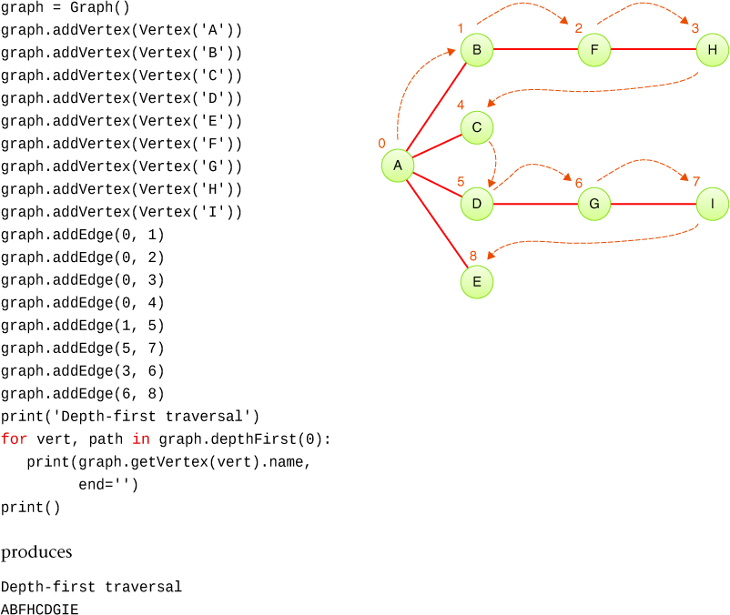
Figure 14-7 A test of depthFirst() on a small graph
Looking back on the choice to yield both the vertex and the path to that vertex in the depthFirst() generator, note the redundancy because the vertex is always the last element in the path. You could rewrite the generator to return only the path, shifting the responsibility of extracting the vertex to the caller. That’s not much of a change in Python where the caller can access the last vertex using an O(1) reference to path[-1]. If the path is returned as a linked list, however, getting the last element takes O(N) time and merits the extra return value.
Depth-First Traversal and Game Simulations
When you’re implementing game programs, depth-first traversal can simulate the sequence of moves made by players. In two-player board games like chess, checkers, and backgammon, each player chooses from among a set of possible actions on their turn. The actions at each turn depend on the state of the game, sometimes called the board state. For example, in the initial state of chess, the actions are limited to movement of the pawns or knights. Subsequent board states allow actions involving the other pieces.
This behavior can be modeled with a graph where the possible actions form edges between board states, which are the vertices in a graph. Starting from a particular board state, depth-first traversal enumerates all possible board states that could be reached from the initial state.
Let’s look at how that works for a simple game of tic-tac-toe. The first player, let’s say it is the X-player, can make one of nine possible moves. The O-player can counter with one of eight possible moves, and so on. Each move leads to another group of choices by your opponent, which leads to another series of choices for you, until the last square is filled. Figure 14-8 shows a partial graph of the board states. Only the edges connecting the topmost board state for each move are included, and symmetric board states are not drawn. That leaves only three distinct possible choices for the X-player’s first move.
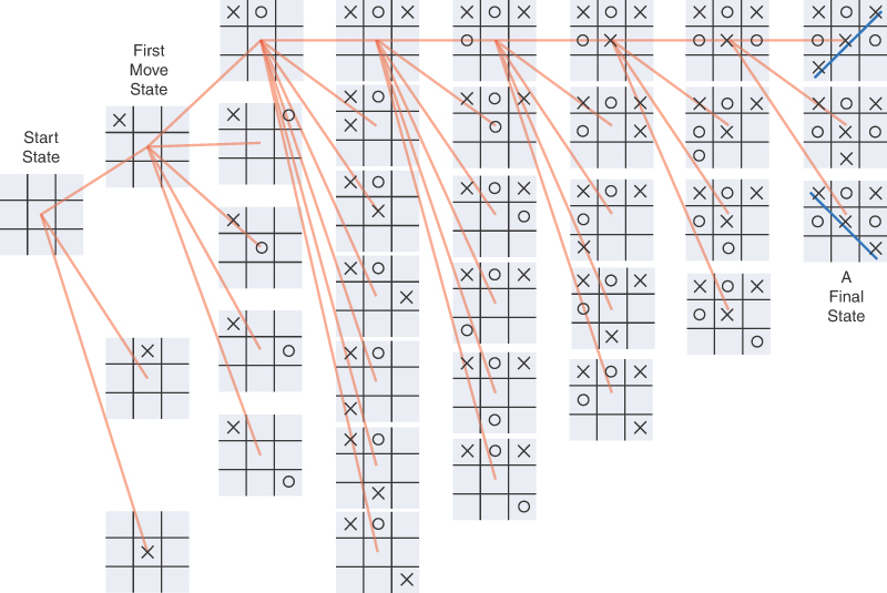
FIGURE 14-8 Tic-tac-toe board states as a graph
When you are deciding what move to make, one approach is to mentally imagine a move, then your opponent’s possible responses, then your responses, and so on. You can decide what to do by seeing which move leads to the best outcome. In simple games like tic-tac-toe, the number of possible moves is sufficiently limited that it’s possible to follow each path to the end of the game.
Analyzing these moves involves traversing the graph. As evident in Figure 14-8, even a “simple” game like tic-tac-toe can lead to a large graph. The number of edges for the first move, after eliminating symmetric moves, is three. The O-player’s first move includes four options. The next X-player move can have up to seven options after eliminating symmetry. The number of options diminishes after that.
Using depth-first traversal means the analysis drives toward the final states first. Any path that leads to an opponent’s victory could be eliminated or, at least, set aside to be further explored as a last option. That would allow you to “prune” the graph significantly. How much could pruning save? If you don’t pay attention to symmetry, there are nine possible first moves, followed by eight possible opponent moves, followed by seven possible first-player moves, and so on. That’s 9×8×7×6×5×4×3×2×1 (9 factorial or 9! or 362,880) moves, ignoring the reduction due to games ending after one player completes three in a row. Those moves are edges in the graph, and that’s a lot of edges to follow. Pruning could make a huge savings.
Although exploring 362,880 edges seems manageable for modern computers, other games have much larger graphs. Chess has 64 squares and 16 pieces for each player. The game of go has a 19-by-19 grid of points where players place either a black or white stone. Those 361 points mean there are something like 361! potential sequences of moves (and that number doesn’t account for the removal and replacement of stones). Even though some of the sequences result in the same board state, exploring the full graph is quite daunting. Most game-playing algorithms only explore the graph to a particular depth and use many techniques to eliminate as many paths as possible in analyzing move options. They may never generate the complete graph.
Breadth-First
The depth-first traversal algorithm acts as though it wants to get as far away from the starting point as quickly as possible. In the breadth-first, on the other hand, the algorithm likes to stay as close as possible to the starting point. It first visits all the vertices adjacent to the starting vertex, and only then goes further afield. This kind of traversal is implemented using a queue instead of a stack.
An Example
Figure 14-9 shows the same graph as Figure 14-5, but this time we traverse the graph breadth-first. Again, the numbers indicate the order in which the vertices are visited. Like before, A is the starting vertex. You mark it as visited and place it in an empty queue. Then you follow these rules:
Rule 1
Take the first vertex in the queue (if there is one) and insert all its adjacent unvisited vertices into the queue, marking them as visited.
Rule 2
If you can’t carry out Rule 1 because the queue is empty, you’re done.
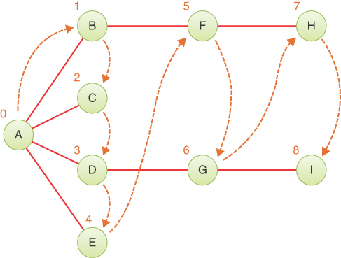
FIGURE 14-9 Breadth-first traversal example
The breadth-first traversal is slightly simpler than the depth-first traversal because there are only two rules. Walking through the example, you first visit A. Then you take all the vertices adjacent to A and insert each one into the queue as you visit and mark it. Now you’ve visited A, B, C, D, and E. At this point the queue (from front to rear) contains BCDE.
You apply Rule 1 again, removing B from the queue and looking for vertices adjacent to it. You find A and F, but A has been visited, so you visit and insert only F in the queue. Next, you remove C from the queue. It has no adjacent unvisited vertices, so nothing is visited or inserted in the queue. You remove D from the queue and find its neighbor G is unvisited, so you visit it and insert it in the queue. You remove E and find no unvisited neighbors.
At this point the queue contains FG, the only adjacent unvisited vertices found while previously visiting BCDE. You remove F and visit and insert H on the queue. Then you remove G and visit and insert I.
Now the queue contains HI. After you remove each of these and find no adjacent unvisited vertices, the queue is empty, so you’re done. Table 14-4 shows this sequence.
Table 14-4 Queue Contents During Breadth-First Traversal
Event | Queue (Front to Rear) |
|---|---|
Visit A | A |
Remove A | |
Visit B | B |
Visit C | BC |
Visit D | BCD |
Visit E | BCDE |
Remove B | CDE |
Visit F | CDEF |
Remove C | DEF |
Remove D | EF |
Visit G | EFG |
Remove E | FG |
Remove F | G |
Visit H | GH |
Remove G | H |
Visit I | HI |
Remove H | I |
Remove I | |
Done |
At each moment, the queue contains the vertices that have been visited but whose neighbors have not yet been fully explored. (Contrast this breadth-first traversal with the depth-first traversal, where the contents of the stack hold the route you took from the starting point to the current vertex.) The vertices are visited by breadth-first in the order ABCDEFGHI.
The Graph Visualization Tool and Breadth-First Traversal
Use the Graph Visualization tool to try out a breadth-first traversal using the Breadth-First Traverse button. Again, you can experiment with the graph in Figure 14-9, or you can make up your own.
Notice the similarities and the differences of the breadth-first traversal compared with the depth-first traversal.
You can think of the breadth-first traversal as proceeding like ripples widening when you drop a stone in water or—for those of you who enjoy epidemiology—as the influenza virus carried by air travelers from city to city. First, all the vertices one edge away from the starting point (plane flight) are visited, then all the vertices two edges away are visited, and so on.
Python Code
The breadthFirst() method of the Graph class is like the depthFirst() method, except that it uses a queue instead of a stack and fully explores the sequence of adjacent unvisited vertices. The implementation for both the Queue class and the traversal generator is shown in Listing 14-5.
LISTING 14-5 The breadthFirst() Traversal Generator for a Graph
class Queue(list):          # Use list to define Queue class
   def insert(self, j): self.append(j) # insert == append
   def peek(self): return self[0] # First element is front of queue
   def remove(self): return self.pop(0) # Remove first element
   def isEmpty(self): return len(self) == 0

class Graph(object):
…
   def breadthFirst(        # Traverse the vertices in breadth-first
         self, n):          # order starting at vertex n
      self.validIndex(n)    # Check that vertex n is valid
      visited = [False] * self.nVertices() # Nothing visited initially
      queue = Queue()       # Start with an empty queue and
      queue.insert(n)       # insert the starting vertex index on it
      visited[n] = True     # and mark starting vertex as visited
      while not queue.isEmpty(): # Loop until nothing left on queue
         visit = queue.remove() # Visit vertex at front of queue
         yield visit        # Yield vertex to visit it
         for j in self.adjacentUnvisitedVertices( # Loop over adjacent
               visit, visited): # unvisited vertices
            queue.insert(j) # and insert them in the queue
Here, we define the Queue class as a subclass of list. Inserting an item in the queue uses the list’s append() method. This means the back (or end) of the queue is at the highest index of the list. That means, peek() and remove() operate on the first element of the list at index 0. The Python list.pop() method takes an optional parameter for the index of the item to remove.
The beginning of the traversal starts off just as it did for depth-first, checking the validity of the starting vertex and creating a visited array for all the vertices. Then the visited array is created and seeded with the starting vertex index, and that index is marked as visited. The implementation in Listing 14-5 deviates slightly from the rules shown earlier in that the visit of the first vertex doesn’t happen until inside the while loop where the rules are applied. Also note that marking vertices in the visited array happens before they are yielded to the caller. The overall breadthFirst() generator “visits” a vertex by yielding it to the caller for processing while keeping the internal visited array to track which vertices it has already put in its queue to process.
The while loop test determines whether Rule 1 or Rule 2 will apply. If it’s Rule 1, the loop body removes a vertex from the front of the queue and immediately visits it by yielding it. The method visits the starting vertex in the same way all the others are visited. Note that we no longer have the stack to provide the path taken to reach this vertex. As a consequence, the breadthFirst() generator yields only a vertex index. It’s possible and useful to provide the path, and we leave that as a programming project.
After breadthFirst() removes a vertex from the queue and visits it, the next thing to do is insert all the adjacent unvisited vertices in the queue. That process is handled by looping through the adjacentUnvisitedVertices() generator (shown in Listing 14-3) and inserting the vertices in the queue. That completes the implementation of Rule 1. Rule 2 is also done because no more processing is needed when the queue is empty.
Let’s test the breadthFirst() traversal on nearly the same graph used for depth-first, but let’s add one edge between C and H to see what effect it has. Figure 14-10 shows the code used to construct the graph and traverse the vertices in breadth-first order. The extra edge is highlighted in the code. Note that the vertex ID numbers used to create the edges are different from the visit numbers next to the vertices in the figure.
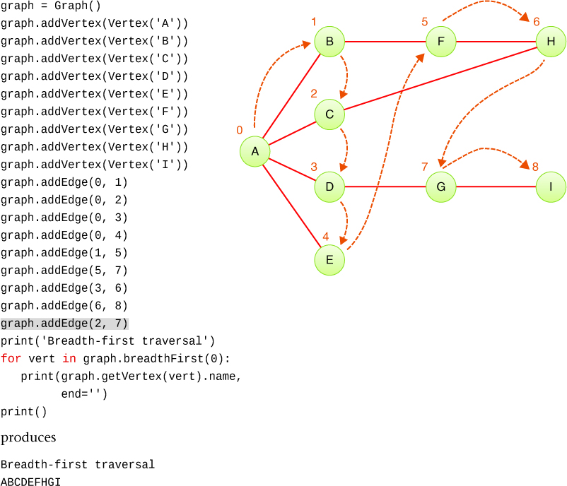
FIGURE 14-10 A test of breadthFirst() on a small graph
In the test example, after visiting ABCDE, the queue contains the unvisited adjacent vertices, FHG. Without the edge from C to H, the queue would have been FG, like in the graph of Figure 14-9. With the edge CH, H is marked as visited and inserted on the queue when C is removed. Then F is removed, and its neighbors searched for unvisited vertices. H has not yet been visited (yielded by the generator that starts at F), but it was marked as visited as it was added to the queue. So, H does not show up as a vertex to add to the queue. The next pass through the while loop removes H from the front of the queue and visits it. Because it, too, has no adjacent unvisited neighbors, nothing is put on the queue. The next pass removes G from the queue, finds I as unvisited, and inserts that final vertex.
This example illustrates an interesting property of breadth-first traversal and search: it first finds all the vertices that are one edge away from the starting point, then all the vertices that are two edges away, and so on. This capability is useful if you’re trying to find the shortest path from the starting vertex to a given vertex (see Project 14.3). You start a breadth-first traversal, and when you visit a particular vertex, you know the path you’ve traced so far is the shortest path to it. If there were a shorter path, the breadth-first traversal would have visited it already. In Figure 14-10, there are two paths from A to H: ABFH and ACH. The fact that breadth-first visits H before G is due to having a two-edge path using the added edge. In Figure 14-9, the absence of edge CH means G is visited before H because both G and H can only be reached through three-edge paths.
Minimum Spanning Trees
Suppose you’re designing a large apartment building and need to decide where the hot water pipes should go. The example shown in Figure 14-4 shows a completed plumbing network for a two-and-a-half-bathroom house, but let’s imagine you have hundreds of sinks, bathtubs, showers, washing machines, and hot water heaters to connect. For the water supply, you could connect every fixture to every other one with a pipe. That would certainly provide the shortest possible path between every pair of fixtures. That would also cost a lot, and any plumber asked to do the installation would probably laugh.
After you get over your embarrassment, you realize that you only really need to connect every sink, bathtub, shower, and washing machine to a water heater. You want those pipes to be short so that the hot water can reach the faucets quickly and to minimize the length of pipe needing insulation. You can’t run the pipes through the rooms of the building; they must be hidden inside the walls, floors, and ceilings. Not every wall will allow pipes to go through it, such as a wall made of glass. So, you must take some twisted paths to hook everything together. How do you find which paths to hook up so that all the fixtures are connected but the amount of pipe is the shortest?
It would be nice to have an algorithm that, for any connected set of fixtures and pipes (vertices and edges, in graph terminology), would find the minimum set of pipes needed to connect all the fixtures. Even if it didn’t find the absolute minimum pipe length overall or the minimum total distance to the water heater, you wouldn’t want any extra pipes connecting two fixtures if there was another path between them. For instance, you wouldn’t want a loop of pipes (edges) like the path ABFHCA in Figure 14-10 or the fully connected graph on the left of Figure 14-11 (although there are cases where plumbing loops are desirable). The result of such an algorithm would be a graph with the minimum number of edges necessary to connect the vertices. The graph on the left of Figure 14-11 has the maximum number of edges, 10, for a five-vertex graph. The graph on the right has the same five vertices but with the minimum number of edges necessary to connect them, four. This constitutes a minimum spanning tree (MST) for the graph.
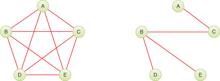
FIGURE 14-11 A fully connected graph and a minimum spanning tree
There are many possible minimum spanning trees for a given graph. The MST of Figure 14-11 shows edges AC, BC, BD, and BE, but edges AC, CE, ED, and DB would do just as well. The arithmetically inclined will note that the number of edges in a minimum spanning tree is always one fewer than the number of vertices. Removing any edge from a minimum spanning tree would create multiple connected components.
For now, don’t worry about the length of the edges. You’re not trying to find a minimum physical length, just the minimum number of edges. (Your plumber might have a different opinion.) We discuss more about this when we talk about weighted graphs in the next chapter.
The algorithm for creating the minimum spanning tree is almost identical to that used for traversing. It can be based on either the depth-first or the breadth-first traversal. This example uses the depth-first traversal.
Perhaps surprisingly, by executing the depth-first traversal and recording the edges you’ve traveled to reach a vertex, you automatically create a minimum spanning tree. It’s also somewhat counterintuitive because breadth-first traversal finds the shortest path to each vertex. The only difference between the minimum spanning tree method, which you see in a moment, and the depth-first traversal, which you saw earlier, is that it must somehow record and return a tree-like structure.
Minimum Spanning Trees in the Graph Visualization Tool
The Graph Visualization tool runs the minimum spanning tree algorithm after you select a starting vertex and select the corresponding button. You see the depthFirst() generator run in the code window to yield results to a method we explore shortly.
As the depth-first traversal yields vertices and their paths from the starting vertex, the Visualization tool highlights them, as shown in Figure 14-12. In the example, the algorithm adds vertex E and its path from the starting vertex, C, to the tree it is building. The vertices that have been added have brown circles around them (B, C, D, and E) and the edges forming the path returned by depthFirst() are highlighted in blue. Edges added in earlier steps (for example, edge BD) are highlighted in brown.
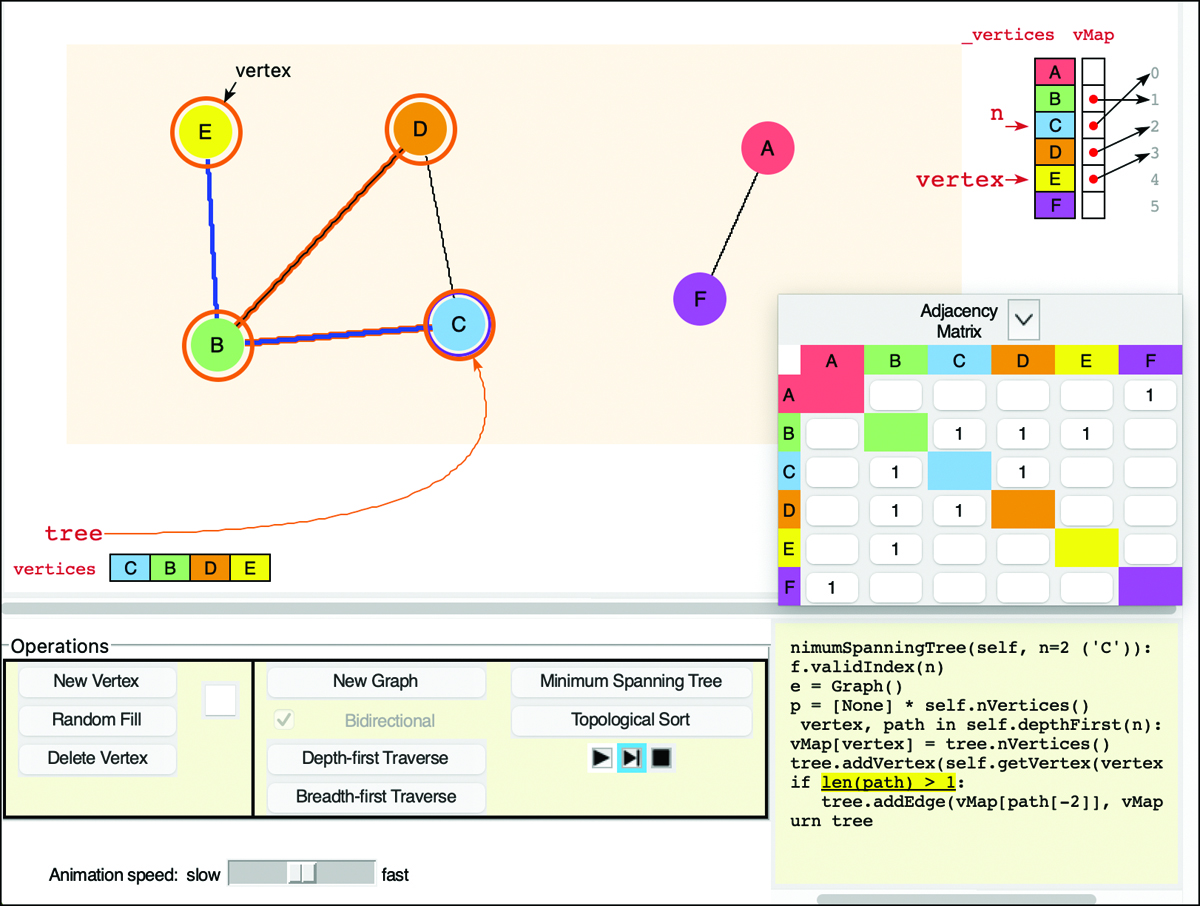
FIGURE 14-12 The Graph Visualization tool adding a path to a minimum spanning tree
As you can see, the minimum spanning tree implementation must track many things as it runs. We explore the detailed implementation in Python, but first we need to revisit a structure that we discussed in detail in several preceding chapters: trees.
Trees Within a Graph
What does a minimum spanning tree “look” like? Is it a binary tree? No, because the number of vertices connected to a given vertex could be one, two, three, and so on. For example, in the minimum spanning tree on the right of Figure 14-13, there is no way to arrange the vertices and edges into a binary tree form. Even though the trees for both Figure 14-11 and Figure 14-13 come from the same starting graph, it’s not possible to know whether the resulting tree will have edges that could form a binary tree.
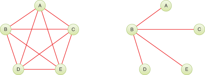
FIGURE 14-13 Another minimum spanning tree from a fully connected five-vertex graph
So, what structure should be used to represent the minimum spanning tree? You could try to make a tree structure with an arbitrary number of children for each node, something like the 2-3-4 tree but with any number of children. That could be a good solution, but there’s an easier one: use the Graph class itself.
A minimum spanning tree is a subgraph—a subset of the original graph’s vertices and edges. The spanning part means that all the vertices in a connected component are still connected, and the tree means there is a single, unique path between every pair of vertices. The trees you’ve seen so far all share those properties. There was a unique path from the root to every node in the tree, and all of them were reachable from the root.
It’s possible for the minimum spanning tree to include every vertex and edge of the input graph. Typically, however, the tree is a proper subset of the vertices and edges forming a connected component.
Python Code for the Minimum Spanning Tree
Our minimumSpanningTree() method returns a new graph with a subset of the vertices and edges in the starting graph. We create the MST using a depth-first traversal from a starting vertex. All the vertices in the connected component that includes the starting vertex will go in the MST. Any nonconnected vertices, like A and F in Figure 14-12, are left out. Listing 14-6 shows the code.
Because the result contains a subset of the original vertices, the vertex indices could be different in the two graphs. For instance, a 10-vertex graph might be composed of two connected components: one with six vertices and the other with four. If you ask for an MST starting from a vertex in the six-vertex component, the MST will have exactly six vertices with indices 0 through 5. Those vertices could have indices up to 9 in the original graph, so you need a way to track the correspondence of vertices in the original graph to those in the MST.
LISTING 14-6 The minimumSpanningTree() Method of Graph
class Graph(object):
…
   def minimumSpanningTree( # Compute a minimum spanning tree
         self, n):          # starting at vertex n
      self.validIndex(n)    # Check that vertex n is valid
      tree = Graph()        # Initial MST is an empty graph
      vMap = [None] * self.nVertices() # Array to map vertex indices
      for vertex, path in self.depthFirst(n):
         vMap[vertex] = tree.nVertices() # DF visited vertex will be
         tree.addVertex(    # last vertex in MST as we add it
            self.getVertex(vertex))
         if len(path) > 1:  # If the path has more than one vertex,
            tree.addEdge(   # add last edge in path to MST, mapping
               vMap[path[-2]], vMap[path[-1]]) # vertex indices
      return tree
The minimumSpanningTree() method starts with an empty graph—called tree—to hold the MST. As we add vertices to it, we note the translation between old and new vertices in an array called vMap. The array needs a cell for every possible vertex. Just before we add a vertex to the MST, we know what index it will get because it’s placed at the end of the existing vertices. That means the old vertex index maps to the number of the vertices added to the MST so far.
To see how the mapping works, look at the sample vMap in Figure 14-12. The vMap appears in the upper right of the display as an array aligned with input vertices whose values point to indices in the new tree (vertex indices). As the starting point, vertex C was visited first and becomes the first vertex in the output tree, so the vMap shows C mapping to index 0. The next vertex added to the tree is vertex B, so it maps to index 1, and so on. Only the vertices included in the minimum spanning tree will have entries in vMap mapping them to their new indices. In Figure 14-12, vertices A and F are not in vMap because they are not connected to C.
In the code after setting up the empty tree and vMap, minimumSpanningTree() uses the depthFirst() traversal over the graph to visit all the vertices in the connected component. The depthFirst() traversal yields both a vertex and the path to the vertex for each visit (in the form of a stack). The first vertex visited will always be the starting vertex, and the path will contain just that one vertex on the visit.
In the depth-first loop body, we first store the mapping from the vertex being visited to its index in the MST. The number of vertices already in the tree provides the index to store in vMap. The next call adds the vertex being visited to the MST. Then, if the path to the visited vertex has at least one edge in it, we add the last edge to the MST as well. We get the vertices forming that edge from the last two vertices in the path: path[-2] and path[-1]. We must translate those vertex indices using the vMap array. We’re guaranteed that the indices in the path were set in vMap because the path contains only vertices that were previously visited by depthFirst().
Does this code handle everything? What about the edges? We add one edge for each vertex added to the MST other than the starting vertex. Is that enough? Yes, adding one edge per vertex means we get exactly the N–1 edges from the N vertex connected component. Each added edge is the last edge in the unique path that leads to that vertex. So, the algorithm covers all the vertices and edges of the connected component that belongs in the MST.
When the depth-first traversal is complete, tree contains the full minimum spanning tree, so it is returned to the caller. To help with development and see the detailed contents of the various arrays, you can define some print methods for the Graph class, as shown in Listing 14-7.
LISTING 14-7 Methods for Summarizing and Printing Graphs
class Graph(object):
…
   def __str__(self):       # Summarize the graph in a string
      nVertices = self.nVertices()
      nEdges = self.nEdges()
      return '<Graph of {} vert{} and {} edge{}>'.format(
         nVertices, 'ex' if nVertices == 1 else 'ices',
         nEdges, '' if nEdges == 1 else 's')

   def print(self,          # Print all the graph's vertices and edges
             prefix=''):    # Prefix each line with the given string
      print('{}{}'.format(prefix, self)) # Print summary form of graph
      for vertex in self.vertices(): # Loop over all vertex indices
         print('{}{}:'.format(prefix, vertex), # Print vertex index
               self.getVertex(vertex)) # and string form of vertex
         for k in range(vertex + 1, self.nVertices()): # Loop over
            if self.hasEdge(vertex, k): # higher vertex indices, if
               print(prefix, # there's an edge to it, print edge
                     self._vertices[vertex].name,
                     '<->',
                     self._vertices[k].name)
These printing methods use some of Python’s string formatting features, which we don’t describe here. Instead, we show what they produce on a small example.
For this example, we use a small graph with six vertices, two of which are not connected to the other four. Figure 14-14 shows the original graph on the left along with the depth-first traversal starting at vertex A. The minimum spanning tree is on the right. Vertices C and F do not appear in the minimum spanning tree because they are not connected by an edge to the other vertices. The output of the print() method appears below each graph. Note that edges are printed once next to their “first” (lower index) vertex and not repeated next to their “second” (higher index) vertex.
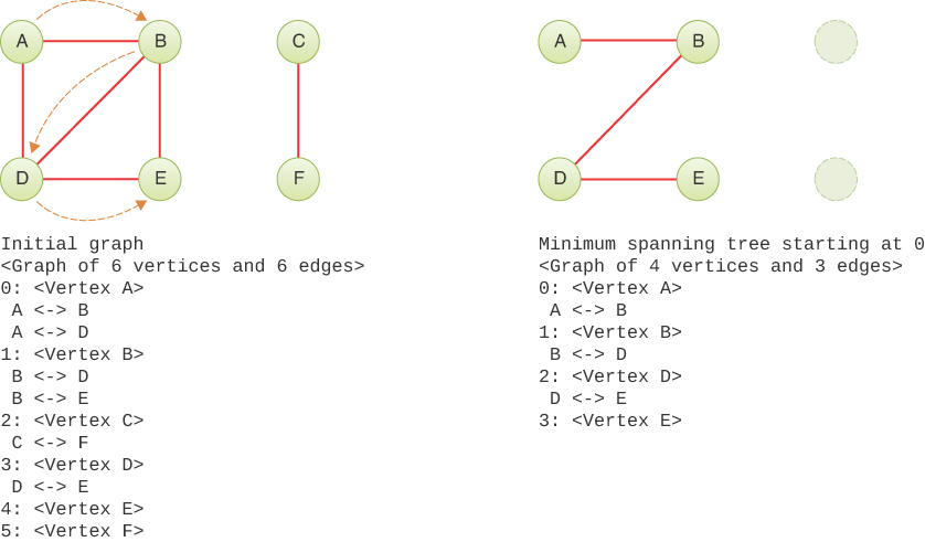
FIGURE 14-14 Printed descriptions of a graph and a minimum spanning tree
The minimum spanning tree algorithm follows the depth-first traversal to get all the vertices in the connected component of the starting vertex. The vertices of other components are ignored. The resulting subgraph will always have N–1 edges for the N vertices in the connected component.
How much time does it take to build the minimum spanning tree? Well, it’s at least O(N) to go through all the N vertices. The depthFirst() traversal method seems as though it should be O(N), as was the case for all the traversal algorithms you’ve seen for other data structures. A closer inspection, however, shows that for each vertex visited, the depthFirst() generator starts up its own internal loop over all vertices to find the first adjacent unvisited one. If there are few edges, that inner loop could go through most of the vertices before finding the next adjacent one. That means it could take O(N) just to find the next adjacent vertex, and depthFirst() traversal could take O(N2). The breadth-first traversal always completes its inner loop, so it’s definitely O(N2). That’s not always going to happen for depth-first, as we discuss in the next chapter, but for now you can assume that worst case and that means the minimum spanning tree takes O(N2) too.
Topological Sorting
Topological sorting is another operation that can be modeled with graphs. It’s useful in situations where items or events must be arranged in a specific order. Let’s look at an example.
Dependency Relationships
In school, students find (sometimes to their dismay) that they can’t take just any course they want. Some courses have prerequisites—other courses that must be taken first. The course sequence usually models a hierarchy where some concepts cannot be mastered without first understanding another set of concepts. These are dependency relationships. They occur everywhere. Algebra depends on understanding arithmetic; linear algebra depends on understanding algebra. In programming, a source file can import or include other source files, which makes one file dependent on another. In cooking, each step depends on completing the previous preparations. For example, baking bread depends on mixing the dough and heating an oven.
Dependency relationships can be described with a graph—specifically a directed graph. Figure 14-15 shows a simplified recipe for baking bread.
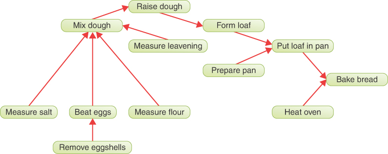
FIGURE 14-15 A dependency graph for baking bread
To bake bread, you need to have a heated oven and a loaf of dough in a pan. To have a loaf, it should be shaped from dough. That dough should be raised first, and so on. Most of the steps must be done in a particular order. Removing the eggshells after beating the eggs would be problematic (removing them after raising the dough would be even worse). Some pairs of steps, however, can be done in either order. It doesn’t matter which order you measure the flour and the salt; and heating the oven and mixing the dough can be done in either order, even simultaneously. The dependency relations shown by the arrows capture this partial ordering.
Analyzing the different tasks and their relative order may seem trivial to anyone who has baked bread before, but they are anything but trivial to a robot. Imagine a robot that could a read a cookbook recipe and figure out all the steps. Assuming it could understand the meaning of the words, it would still need to determine the ordering of tasks. Recipes are usually written in chronological order of the steps, so it could simply follow that sequence. That, however, would probably lengthen the preparation time because steps that could be done at the same time would be done sequentially. Ideally, it would analyze all the possible orderings of the steps and find the most efficient one.
Directed Graphs
Dependency relationships expose a graph feature we haven’t discussed yet: the edges need to have a direction. When this is the case, the graph is called a directed graph or a digraph. In a directed graph you can proceed only one way along an edge. The arrows in Figure 14-16 show the direction of the edges.
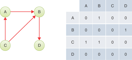
FIGURE 14-16 A small directed graph and its adjacency matrix
In a program, the difference between an undirected graph and a directed graph is that an edge in a directed graph has only one entry in the adjacency matrix. Figure 14-16 shows a small directed graph and its adjacency matrix.
Each 1 in the matrix represents a single edge. The row labels show where the edge starts, and the column labels show where it ends. Thus, the edge from A to B is represented by a single 1 at row A column B. If the directed edge were reversed so that it went from B to A, there would be a 1 at row B column A instead.
For an undirected graph, as noted earlier, half of the adjacency matrix mirrors the other half, so half the cells are redundant. For directed graphs, however, every cell in the adjacency matrix conveys unique information. The halves are not mirror images.
For a directed graph, the method that adds an edge thus needs only a single statement
self._adjMat[A, B] = 1
instead of the two statements required in an undirected graph. If you use the adjacency-list approach to represent your graph, then A has B in its list, but—unlike an undirected graph—B does not have A in its list.
Sorting Directed Graphs
Imagine that you make a list of all the actions needed to bake bread, using Figure 14-15 as your input data. You then arrange the actions in the order you need to take them. The final Bake bread step (Bb) is the last item on the list, which might look like this using two initials for each vertex:
Mf,Ms,Ml,Re,Be,Md,Rd,Fl,Pp,Pl,Ho,Bb
Arranged this way, the graph vertices are said to be topologically sorted. Any action you must take before some other action occurs before it in the list.
Many possible orderings would satisfy the dependency relationships. You could heat the oven and prepare the pan first as in
Ho,Pp,Mf,Ms,Ml,Re,Be,Md,Rd,Fl,Pl,Bb
This approach also satisfies all the relationships (although the similarity to chemical symbols might be a bit unsettling when thinking about bread). There are many other possible orderings as well. When you use an algorithm to generate a topological sort, the approach you take determines which of various valid sortings are generated. The specific constraint that must be followed in graph terminology is as follows. For it to be a valid sorting of a directed graph, if there is a path from vertex A to vertex B, vertex A must precede vertex B in the topological sort.
Directed graphs can model other situations besides recipe steps and course prerequisites. Many industrial projects are managed by breaking down the overall project into smaller jobs or tasks. Each task might depend on outputs of other tasks and might require some time to elapse between the end of one task and the start of another. Take building a house as an example. The person who wants the house constructed must identify a site, find a builder, obtain permits, and get financing. The actual construction work depends on having all those tasks done. There could be a delay between completing all the preparation tasks and commencing construction as the builder finds crewmembers available to start the new work. These delays are somewhat predictable, but rarely with any precision.
Modeling job schedules with graphs is called critical path analysis. Although we don’t show it here, a weighted, directed graph (discussed in the next chapter) can be used, which allows the graph to include the time necessary to complete different tasks in a project. The graph can then tell you such things as the minimum time necessary to complete the entire project and overall costs by looking at different possible topological sorts.
The Graph Visualization Tool
The Graph Visualization tool can model directed graphs too. When the graph has no edges, you can select or clear the Bidirectional checkbox. The checkbox is disabled when any edges exist. You can select New Graph to clear all the vertices and edges and uncheck the Bidirectional box.
The vertices and edges are edited in the same way for directed graphs. The differences are that edges are drawn as a curve with arrow heads; dragging the pointer from one vertex to another only creates the edge from the first one to the second, and clicking a cell in the adjacency matrix only creates the edge from the corresponding row to the corresponding column. Figure 14-17 shows the same directed graph as the bread baking example from Figure 14-15 using the two-letter abbreviations for the operations. The vertices have been rearranged but the edges connecting them remain the same. The adjacency matrix is large and obscures the table of vertices. Use the collapse and uncollapse button to switch the view of the matrix.
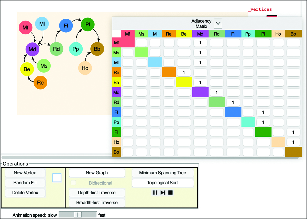
FIGURE 14-17 A directed graph in the Graph Visualization tool.
You can use the tool to run depth and breadth-first traversals and minimum spanning trees of directed graphs. The results are different than for the undirected graphs because the edges are now directional.
The Topological Sorting Algorithm
Let’s look at how to sort the vertices topologically. Here, we start with a basic algorithm and then improve it. For the basic algorithm, we need at least two steps.
Step 1
Find an unvisited vertex that has no (unvisited) predecessors.
The predecessors to a vertex, V, are those vertices that are directly “upstream” from it—that is, connected to it by an edge that points to V. If an edge points from A to B, then A is a predecessor to B (and B is a successor to A). In Figure 14-16, the only vertex with no predecessors is C. In the bread baking example of Figure 14-17, six vertices have no predecessors: Mf, Ms, Ml, Re, Pp, and Ho. These vertices can be found by looking for columns in the adjacency matrix with no edges.
Step 2
Mark the vertex found in Step 1 as visited and add it at the end of the result list.
Steps 1 and 2 are repeated until all the vertices are gone. At this point, the result list holds the vertices arranged in topological order.
You can see the process at work by using the Graph Visualization tool. Construct the graph in Figure 14-16 (or any other graph, if you prefer). Then select the Topological Sort button. There’s no need to select a starting vertex because the algorithm doesn’t need one.
The animation in the Visualization tool proceeds in two phases. It’s a bit fancier than the two-step algorithm shown earlier, but those same steps are used. We look at a couple of different implementations later to see how to sort the vertices efficiently.
Note that this topological sorting algorithm works on unconnected graphs as well as connected graphs. This models the situation in which you have two unrelated goals, such as getting a degree in mathematics and at the same time taking a hiking trip in the mountains. Some graphs, however, cause problems.
Cycles and Trees
One kind of graph that this basic algorithm cannot handle is a graph with cycles. We mentioned how the minimum spanning tree of a graph never creates a loop connecting a vertex to itself by a path of two or more edges. The formal name for such a loop is a cycle.
If a path ends up at the vertex where it started by following directed edges, the graph has at least one cycle. In Figure 14-18 the path BDCB forms a cycle. In addition, ABDCA forms a cycle. Notice that ABCA is not a cycle because you can’t go from B to C in this directed graph.
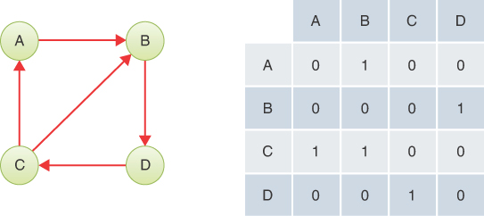
FIGURE 14-18 Directed graph with cycles.
A cycle models the paradox (which some students claim to have encountered at certain institutions), in which course B is a prerequisite for course D, D is a prerequisite for C, and C is a prerequisite for B. Fortunately, such paradoxes are rare.
Cycles can occur in undirected graphs too, but you must be more specific about them. You can typically ignore the cycle formed by following an edge and returning immediately back along the same edge. Cycles must be formed by paths of two or more distinct undirected edges. Multigraphs allow a pair of vertices to be connected by multiple edges, so a cycle could form with as few as two edges. In non-multigraphs, you need at least three undirected edges to form a cycle.
It’s easy to figure out whether some kinds of undirected graphs have cycles. If a graph with N vertices has more than N–1 edges, it must have cycles. You can make this point clear to yourself by trying to draw a graph with N vertices and N edges that does not have any cycles. On the other hand, detecting cycles in directed graphs and graphs with fewer edges can be hard to do. In Chapter 15, “Weighted Graphs,” the section on efficiency discusses the complexity of finding certain kinds of cycles.
An undirected graph with no cycles is always a tree. It’s the presence of cycles that allows two vertices to be connected by distinct paths.
The binary and multiway trees you saw in earlier chapters of this book are types of directed graphs because the edges always link a parent node to a child node. We never allowed those trees to create cycles. Doing so would cause problems like those described for circular lists in Chapter 5.
Topological sorts succeed only on directed graphs with no cycles. Such a graph is called a directed acyclic graph, often abbreviated DAG. The basic topological sorting algorithm doesn’t have a step for what to do if Step 1 fails—when there is no vertex that has no unvisited predecessors. For example, if you ask it to process the graph in Figure 14-18, Step 1 will see that all vertices have at least one predecessor and fail. Thus, we need to add a final step:
Step 3
After Step 1 fails, if the result list has fewer vertices than the graph, the graph must have a cycle.
This three-step algorithm can handle all directed graphs with and without cycles.
Python Code for the Basic Topological Sort
We introduce some new methods in the Graph class to work on predecessors and use them to implement the three steps of the basic topological sorting algorithm in Listing 14-8. The first method, predecessorVertices(), is a generator like adjacentVertices(), which yields all the predecessor vertices of a given vertex, n. It validates the vertex index and then loops over all possible indices, yielding only those with an edge pointing to n.
To implement Step 1, we need a test to find an unvisited vertex with no unvisited predecessors. In other words, the algorithm seeks a vertex where all its predecessors, if any, are among the visited vertices. The onlyVisitedPredecessors() method takes a vertex index, n, as a parameter and uses Python’s all() function to test whether all of n’s predecessors satisfy the condition. The arguments to the all() function are the values of the visited array for each predecessor index. If one or more of those predecessors have a visited value of None or False, then vertex n fails the test. Notably, if n has no predecessors, the argument list to the all() function is empty and it returns True.
LISTING 14-8 Code for the Basic Topological Sort of Vertices
class Graph(object):
…
   def predecessorVertices( # Generate a sequence of vertex indices
         self, n):          # that are adjacent predecessors to n
      self.validIndex(n)    # Check that vertex index n is valid
      for j in self.vertices(): # Loop over all other vertices
         if j != n and self.hasEdge(j, n): # If other vertex connects
            yield j         # via edge, yield other vertex index

   def onlyVisitedPredecessors( # Test whether vertex n's predecessors
         self, n, visited): # have all been visited, if any
      return all(visited[j] # All predecessors must have been set in
                 for j in self.predecessorVertices(n)) # visited array

   def findUnvisitedWithoutPredecessor( # Find a vertex without
         self, visited):    # unvisited predecessor vertices, if any
      for vertex in self.vertices(): # Loop over all vertices
         if (not visited[vertex] and # If vertex is unvisited and has
             self.onlyVisitedPredecessors( # only visited
                vertex, visited)): # predecessors,
            return vertex   # then return it
      return None           # Otherwise there's a cycle or no vertices

   def sortVerticesTopologically( # Return a sequence of all vertex
         self):             # indices sorted topologically
      result = []           # Result list of vertices
      nVertices = self.nVertices() # Number of vertices
      visited = [None] * nVertices # Array to mark visited vertices
      while len(result) < nVertices: # Loop until all vertices handled
         vertex = self.findUnvisitedWithoutPredecessor( # Find an
               visited)     # unvisited vertex without predecessors
         if vertex is None: # If no such vertex exists, then raise an
            raise Exception('Cycle in graph, cannot sort') # exception
         result.append(vertex) # Append unvisited vertex and
         visited[vertex] = True # mark it as visited
      return result
The findUnvisitedWithoutPredecessor() method performs Step 1, looping over all possible vertices, skipping visited vertices, and returning the first unvisited one that satisfies onlyVisitedPredecessors(). If it completes the loop without finding an unvisited vertex without predecessors, it returns None, signaling that there must be a cycle.
The sortVerticesTopologically() method performs Steps 1, 2, and 3. It sets up an empty result list to hold the sorted vertices. Next it creates a visited array, like the ones used in the traversal methods, marking all the vertices as unvisited. The main work begins with the while loop. On each pass of the loop, it tries Step 1 to find a vertex with no predecessors. If that comes back as None, it raises an exception to signal the detection of a cycle. Otherwise, it adds the vertex to the end of the result and marks it as visited, which implements Step 2. If the loop finishes, then there are nVertices in the result list, and it is returned, handling Step 3.
The basic topological sort algorithm is easy to understand, but let’s look at its efficiency. Figure 14-19 shows the different levels of the algorithm. Each level represents one of the methods being called. Let’s look at the innermost level first. Every loop through the vertices() sequence is, of course, O(N). Thus, one call to the onlyVisitedPredecessors() test for a particular vertex looks at all the other vertices, so it takes O(N) time too. At the next level, outward, the findUnvisitedWithoutPredecessor() method calls the inner test on every vertex until it finds one that matches. Although that middle level does quit when it finds such a vertex, it still has to scan some fraction of the vertices, so the combined worst-case complexity of the middle level is O(N2) (to be thorough, we would need to determine the average number of tries needed to find the vertex, but we can assume it’s proportional to N without knowing anything about the graph’s edges).
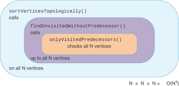
FIGURE 14-19 Complexity of the basic topological sort algorithm
The outermost routine, sortVerticesTopologically(), calls the middle level until all nVerticies have been copied. That’s another O(N) factor, so each level of the algorithm contributes O(N) as shown. Overall, the algorithm is O(N3). Can we do better than that?
Improving the Topological Sort
Yes, we can reduce that complexity to at least O(N2), but it will take a more complicated organization of the data. While this transformation is complicated, learning from examples of how others have improved algorithm performance will help you analyze and improve your own programs. It’s another case study in how to select and use the data structures most appropriate for a task.
The key concept that we’re interested in is the number of edges for each vertex. If we organize the vertices by the number of inbound edges, we can quickly find the ones with no predecessors. In graphs, the number of inbound and outbound edges are called the inbound degree and the outbound degree, or indegree and outdegree, for short.
The first thing we need is a method to get the inbound and outbound degree of a vertex. The degree() method in Listing 14-9 takes a vertex as a parameter, counts both kinds of edges at that vertex, and returns the counts as a tuple.
After we know the inbound degree for all the vertices, we can put all the vertices with degree 0 in one place, so they are easy to find. In fact, if we keep an array indexed by degree, we can put each vertex in the cell of the array for its inbound degree. We need some structure in each array cell that can hold a group of vertices. Should that structure be a stack? A queue? A tree? The answer depends on how we process the vertices, so let’s look at the remaining steps.
After we take a vertex out of the cell for degree 0, we can put it in the sorted result list. The successors of that vertex now have one fewer inbound edge, effectively. A successor that had only one inbound edge from the vertex that was put in the result list can now be considered to have degree 0. So instead of tracking which vertices have been visited, we can simply change the degree for each successor vertex, moving it to the proper cell in the array for its new degree. As we process vertices and their successors, every vertex will eventually be moved down to degree 0 (if there are no cycles).
Knowing that we want to move vertices between cells in the array, it becomes clear that we need a structure that enables fast insertion and deletion. Stacks and queues have O(1) insert and delete complexity, but only for specific orders (LIFO and FIFO). For this algorithm we would need to, say, remove vertex 27 from one cell and add it to another.
If we want to insert and delete items by a key, such as their vertex index, the best data structures would be an array or a hash table. Both have O(1) insert and delete times (assuming we don’t need to shift items in the array to eliminate holes). The hash table has the added advantage of only needing memory proportional to the items in it; an array would need N cells to hold any of the N vertices.
Figure 14-20 illustrates the relations of structures we need. The left side shows a simple four-vertex graph. Next on its right is the Graph object that holds the _vertices array and _adjMat adjacency matrix to represent it. Next to that is a four-element array that shows the inbound degree for each of the four vertices. For example, vertex A has inbound degree 1 while vertex B has inbound degree 2.
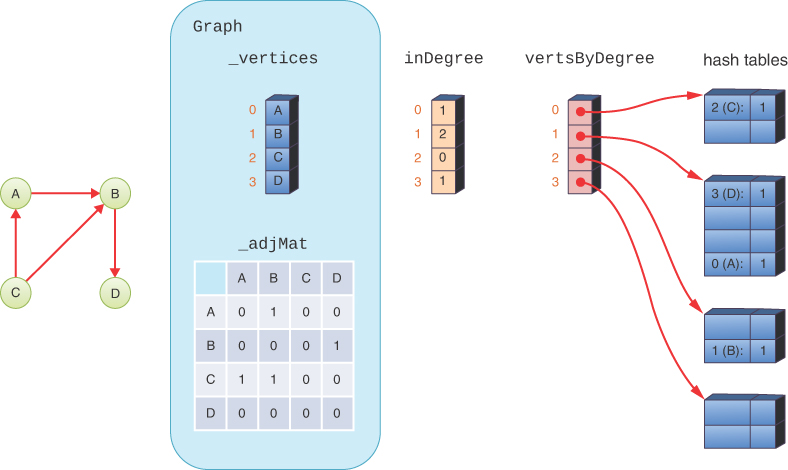
FIGURE 14-20 Structures used for topological sort
The vertsByDegree array groups together the vertices by their inbound degree. Each cell in this array references a hash table that holds the keys for the vertices with a particular inbound degree. For example, vertsByDegree[1] references a hash table holding two keys. The keys are the vertex indices of vertices of inbound degree one: 0 (A) and 3 (D). The hash table for degree three is empty because none of the vertices have inbound degree three. The hash tables have extra cells to maintain a 50 percent load factor.
The sortVertsTopologically() method in Listing 14-9 starts by creating the vertsByDegree array. The maximum inbound degree any vertex could ever have is the number of vertices minus one. For a graph with E edges, the highest inbound edge count could be E. To account for vertices with indegree 0, we need to add 1 to E. The size of the array is the minimum of these values: nVertices and nEdges+1. The vertsByDegree array is built using a list comprehension [{} for j in range(min(self.nVertices(), self.nEdges() + 1))]. As you saw for building the adjacency matrix, using the list comprehension ensures that N distinct empty hash tables are made to fill the array cells.
The sorting algorithm creates an inDegree array to hold the inbound degree of every vertex. Initially, these are filled with 0s.
Now we can populate the new data structures. The next section is a for loop over all the vertices. It calculates the degree of the vertex by calling self.degree() and extracts the first element of the returned tuple using [0] to get the inbound degree.
The sorting algorithm now inserts the vertex in the vertsByDegree array based on its inbound degree. It finds the appropriate hash table by referencing vertsByDegree[inDegree[vertex]]. This kind of nested reference looks a little complicated, but it really is only two array lookups. The vertex variable indexes the inDegree array to get a numeric degree for the vertex. That numeric degree indexes the vertsByDegree array. The content of that array cell is a hash table. To enter a key in a hash table, ht, you could write ht[key] = 1. That’s what’s being done by writing vertsByDegree[inDegree[vertex]][vertex] = 1; it sets the vertex key in the hash table retrieved from vertsByDegree. These strings of references can be tricky to understand when you first look; try working from inner to outer references as well as outer to inner.
LISTING 14-9 The Improved Topological Sort of Vertices
class Graph(object):
…
   def degree(self, n):     # Get degree of vertex as (in, out) pair
      self.validIndex(n)    # Validate vertex index
      inb, outb = 0, 0      # Count inbound and outbound edges
      for j in self.vertices(): # Loop over all vertices
         if j != n:         # other than target vertex
            if self.hasEdge(j, n): # If other vertex precedes
               inb += 1            # increase inbound degree
            if self.hasEdge(n, j): # If other vertex succeeds n
               outb += 1           # increase outbound degree
      return (inb, outb)    # Return inbound and outbound degree

   def sortVertsTopologically( # Return sequence of all vertex indices
         self):             # sorted topologically more efficiently
      vertsByDegree = [     # Make an empty hash table for every
         {} for j in range( # possible degree, max = nVerts – 1 or
            min(self.nVertices(), self.nEdges() + 1))] # nEdges
      inDegree = [0] * self.nVertices() # Allocate indegree array
      for vertex in self.vertices(): # Loop over all vertices, record
         inDegree[vertex] = self.degree(vertex)[0] # inbound degree
         vertsByDegree[     # In hash table for this inbound degree
            inDegree[vertex]][vertex] = 1 # insert vertex
      result = []           # Result list is initially empty
      while len(            # While there are vertices with inbound
            vertsByDegree[0]) > 0: # degree of 0
         vertex, _ = vertsByDegree[0].popitem() # take vertex out of
         result.append(vertex) # hash table & add it to end of result
         for s in self.adjacentVertices( # Loop over vertex's
               vertex):     # successors; move them to lower degree
            vertsByDegree[ # In hash table holding successor vertex
               inDegree[s]].pop(s) # delete the successor
            inDegree[s] -= 1 # Decrease inbound degree of successor
            vertsByDegree[ # In hash table for lowered inbound degree
               inDegree[s]][s] = 1 # insert modified successor
      if len(result) == self.nVertices(): # All vertices in result?
         return result      # Yes, then return it, otherwise cycle
      raise Exception('Cycle in graph, cannot sort')
After the vertsByDegree array is populated with all the vertices and an empty result list/array created, the algorithm can now process the vertices in a while loop. The loop condition tests whether the hash table for inbound degree 0 vertices has any keys in it. If there are no degree 0 vertices, then we’re either done, or the graph has at least one cycle in it.
Inside the while loop body, we pop one of the degree 0 vertices out of its hash table. Python has several methods for removing items from hash tables. The popitem() method removes and returns a key and its value from the hash table. In this case, the sorting algorithm doesn’t care which key is removed, nor what value it has, so it puts the value in the underscore (_) variable. (Python’s popitem() always removes the last key inserted, making it behave like a stack.) Another way to remove a key from a hash table is to use the pop() method, which requires a specific key.
Next, the algorithm appends the degree 0 vertex to the result list. Because the vertex has no predecessors, it can be the next vertex in the output sequence. That allows each of the vertex’s successors to reduce their inbound degree by one. The inner for loop goes through the adjacent vertices of vertex, which are the same as the successors for directed graphs. Each successor vertex, s, is removed from the hash table holding s based on its current degree. The vertsByDegree[inDegree[s]] looks up the hash table and the .pop(s) removes the successor’s key. Next, the algorithm lowers the degree for s by one, and s is inserted in the hash table for that lower degree. After all the successors have been lowered by one degree, the algorithm continues the outer while loop, popping vertices out of the degree 0 hash table.
When the degree 0 hash table is empty, we check the length of the result list against the number of vertices. If the result contains all the vertices, it can be returned as the sorted vertex list. If not, a cycle prevented finding a vertex without predecessors.
Try looking at the details of a topological sort using the Graph Visualization tool. It implements this improved algorithm and shows how the inDegree and vertsByDegree arrays are constructed and updated. As the sortVertsTopologically() method executes, try to figure out what will happen next at each step. The hash tables are shown as simple lists rather than as arrays with empty cells that would illustrate their load factors, but that is not critical to understanding the overall algorithm.
Efficiency of the Topological Sort
Does this new structure—an array of hash tables—improve the efficiency? Let’s review. Building the initial, empty vertsByDegree array takes O(N) time. The first for loop will also take at least O(N) time because it goes through all the vertices. Now we must look at what happens inside that loop.
The call to self.degree(vertex) takes O(N) time because it has to check all N vertices to see whether they have inbound or outbound edges to the given vertex. Thus, populating the inDegree array makes the overall for loop take O(N2) time because it covers the entire two-dimensional adjacency matrix to compute all of these.
We also must examine the statement that puts the vertices in their appropriate hash table inside the vertsByDegree array. It does two array lookups (one inside inDegree and the other inside vertsByDegree) and a hash table access for every vertex. The lookups and the hash table access are all O(1), so this doesn’t add more complexity to the first for loop; overall it takes O(N2) time.
The main while loop of the sortVertsTopologically() method executes N times (if there are no cycles, and fewer if there are any). Inside the loop, the act of popping an item and inserting it at the end of the result list is O(1). The inner for loop must process each of the successors. Finding the (adjacent) successors takes O(N) time, so the inner for loop is at least O(N). Some subset of those N vertices will be successors, and each gets popped from a hash table, decremented in degree, and inserted in another hash table, which are all O(1) operations. The inner for loop takes O(N) time; thus, the outer, main while loop combined with it, takes O(N2) time.
Both preparing the array of hash tables in the first for loop and processing the result in the main while loop take O(N2) time. The extra memory needed for the vertsByDegree and inDegree arrays has made an improvement over the O(N3) time of the basic algorithm. That might seem small, but it can be huge when N grows large.
Connectivity in Directed Graphs
You’ve seen how, in a undirected graph, you can find all the vertices that are connected by doing a depth-first or breadth-first traversal. When you try to find all the connected vertices in a directed graph, things get more complicated. You can’t just start from a randomly selected vertex and expect to reach all the other connected vertices.
Consider the small, directed graph in Figure 14-16 and Figure 14-20. If you start on A, you can get to B and D but not to C. If you start on B, you can get only to D, and if you start on D, you can’t get anywhere. The meaningful question about connectivity is: What vertices can you reach if you start on a particular vertex?
The Connectivity Matrix
You can easily use the depthFirst() method (Listing 14-4) to traverse part of the graph starting from each vertex in turn. For the graph of Figure 14-16, the output will look something like this:
ABD
BD
CABD
D
This is the connectivity table for the directed graph. The first letter is the starting vertex, and subsequent letters show the vertices that can be reached (either directly or via other vertices) from the starting vertex.
Transitive Closure and Warshall’s Algorithm
In some applications it’s important to find out quickly whether one vertex is reachable from another vertex. This is the essential question in genealogy: Who are my ancestors? Another example is a celebrity connection game such as the “six degrees of Kevin Bacon,” where people try to find a path through acquaintances to reach a particular person. Some people hypothesize that you need at most a path length of six acquaintances to reach a celebrity. In many applications the path length doesn’t matter. Perhaps you want to take a trip by train from Athens to Kamchatka, and you don’t care how many intermediate stops you need to make. Is this trip possible? Graphs are ideal for answering these questions. The trip won’t be possible unless the vertices are part of the same connected component.
You could examine the connectivity table, but then you would need to look through all the entries on a given row, which would take O(N) time (where N is the average number of vertices reachable from a given vertex). But you’re in a hurry. Is there a faster way?
It’s possible to construct a table that will tell you quickly (that is, in O(1) time) whether one vertex connects to another. Such a table can be obtained by systematically modifying a graph’s adjacency matrix. The graph represented by this revised adjacency matrix is called the transitive closure of the original graph. Such a revised matrix can be called the connectivity matrix.
Remember that in an ordinary adjacency matrix the row number indicates where an edge starts, and the column number indicates where it ends. The connectivity matrix has a similar arrangement, except the path length between the two vertices may be more than one. In the adjacency matrix, a 1 or True at the intersection of row C and column D means there’s an edge from vertex C to vertex D, and you can get from one vertex to the other in one step. Of course, in a directed graph it does not follow that you can go the other way, from D to C.
You can use Warshall’s algorithm named for Stephen Warshall to find the transitive closure of the graph. It changes the adjacency matrix into a connectivity matrix. This algorithm does a lot in a few lines of code. It’s based on a simple idea:
If you can get from vertex L to vertex M, and you can get from M to N, then you can get from L to N.
A two-step path is thus derived from two one-step paths. The adjacency matrix shows all possible one-step paths, so it’s a good starting place to apply this rule.
You might wonder whether this algorithm can find paths of more than two edges. After all, the rule only talks about combining two one-edge paths into one two-edge path. As it turns out, the algorithm can build on previously discovered multiedge paths to create paths of arbitrary length. The basic idea is: if you can build the connectivity matrix for one and two edge paths, then you could apply the same algorithm to that table to build all the three-edge and fewer paths. If you keep reapplying the algorithm, you will eventually discover all the possible paths.
Here’s how it works. Let’s use the adjacency matrix of Figure 14-21 as an example. For this example, you examine every cell in the adjacency matrix, one row at a time.
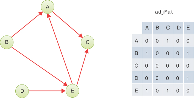
FIGURE 14-21 A five-vertex directed graph and its adjacency matrix
Row A
Let’s start with row A. There’s nothing (0) in columns A and B of that row, but there’s a 1 at column C, so you can stop there.
Now the 1 at this location says there is a path from A to C. If you knew there was a path from some other vertex, X, to A, then you would know there was a path from X to C. Where are the edges (if any) that end at A? They’re in column A. So, you examine all the cells in column A. In the _adjMat of Figure 14-21, there’s only one 1 in column A: at row B. It says there’s an edge from B to A. So, you know there’s an edge from B to A, and another (the one you started with when examining row A) from A to C. From this, you infer that you can get from B to C in two steps. You can verify this is true by looking at the graph.
To record this result, you put a 1 at the intersection of row B and column C. The result is shown in the second matrix in Figure 14-22. The highlighted cell shows where the value changed to 1.
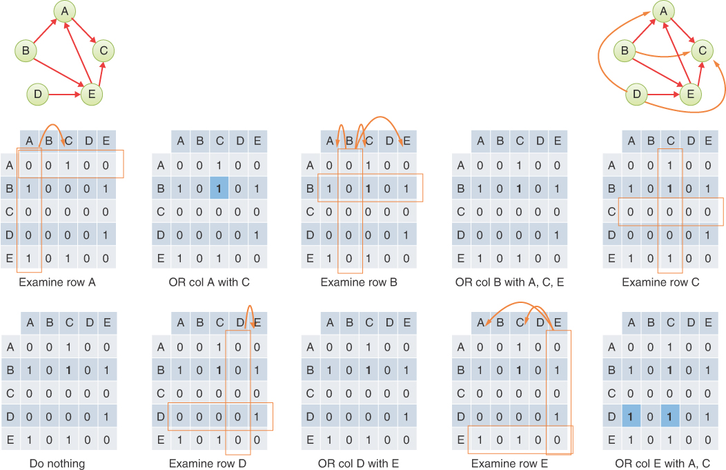
FIGURE 14-22 Steps in Warshall's algorithm
The remaining cells of row A are blank. You only need to copy the contents of column A to columns that have a 1 in row A. In other words, you perform an operation akin to a bitwise OR of column A and column C for this first “bit” that you find turned “on”. Note that column A also has a 1 for vertex E. Column C already had a 1 for vertex E, so the bitwise OR operation doesn’t change it.
Rows B, C, and D
Next, you go to row B. The first cell, at column A, has a 1, indicating an edge from B to A. Do any edges end at B? You look in column B, but it’s empty, so you know that none of the 1s you find in row B will result in finding longer paths because no edges end at B. You could perform the bitwise OR of column B with the three columns that have a 1 in row B, but a bitwise OR with 0s doesn’t change anything, as shown in the fourth panel of Figure 14-22.
Row C has no 1s at all, so you go to row D. Here, you find an edge from D to E. Column D is empty, however, so no edges end on D and the OR changes nothing.
Row E
In row E you see there are edges from E to A and from E to C. Looking in column E, you see the first entry is for the edge B to E, so with B to E and E to A, you infer there’s a path from B to A. That path, however, has already been discovered, as indicated by the 1 at that location.
There’s another 1 in column E, at row D. This edge from D to E plus the ones from E to A and E to C imply paths from D to A and C, so you insert a 1 in both of those cells. The result is shown in last matrix of Figure 14-22.
Warshall’s algorithm is now complete. You’ve added three 1s to the adjacency matrix, which now shows which vertices are reachable from another vertex in any number of steps. The graph at the top right of Figure 14-22 shows the edges added to the graph by the transitive closure as curved arrows in a different color.
Long Paths
Can Warshall’s algorithm find long paths in the graph and build the full closure? It seems as though going row by row once through the matrix might not find long, complicated chains of edges. Figure 14-23 shows a longer example.
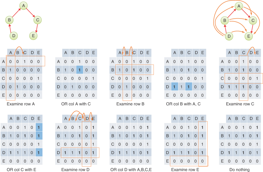
FIGURE 14-23 Warshall's algorithm on a long path
In this graph, the five vertices are connected by four edges to form a long chain. Each step of Warshall’s algorithm adds new edges to the matrix. First, one edge is added for row A, then two edges when it examines row B, and then three edges for row C. The new entries sometimes line up in a column and sometimes in a row. The six edges are all that are needed to build the final connectivity matrix; rows D and E contribute nothing because either the row or its corresponding column contains all 0s.
Cycles
If D were connected to E in the graph of Figure 14-23, it could form a cycle, assuming the direction of the edge went from E to D. What happens in the connectivity matrix if there’s a cycle? Does Warshall’s algorithm still work?
In fact, Warshall’s algorithm can be used to detect cycles. Consider the example shown in Figure 14-24. Vertices A, B, C, and D form a cycle with vertex E dangling from vertex C. In the initial adjacency matrix, which is the upper-left matrix in the figure, the identity diagonal where the row index is the same as the column index has all 0s. That’s what you expect in adjacency matrices because only pseudographs to allow vertices to have edges to themselves.
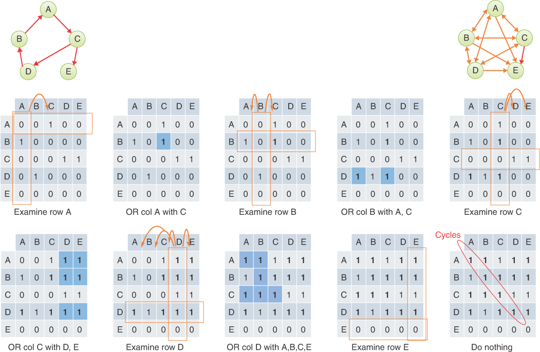
FIGURE 14-24 Warshall's algorithm applied to a graph with a cycle
If you go through the steps of Warshall’s algorithm, the final connectivity matrix shows all 1s along the diagonal except for vertex E (as circled in the matrix at the bottom right of Figure 14-24). That means vertices A, B, C, and D must be part of at least one cycle. There is some path starting from each vertex that leads back to itself.
The presence of 1s along the diagonal tells you that cycles must exist, but not how many there are nor which vertices are in which cycles. Those are harder problems to solve. Nevertheless, it’s useful to have methods that identify the presence (and absence) of cycles. The 0 in the diagonal entry for vertex E in Figure 14-24 tells you that it is not part of a cycle. (Perhaps schools should be required to check for 0s by applying this to the dependency relationship graph of all their course prerequisites.)
Implementation of Warshall’s Algorithm
One way to implement Warshall’s algorithm is with three nested loops (as suggested by Sedgewick; see Appendix B, “Further Reading”). The outer loop looks at each row; let’s call its variable R. The loop inside that looks at each cell (column) in the row; it uses variable C. If a 1 is found in matrix cell (R, C), there’s an edge from R to C, and then a third (innermost) loop is activated.
The third loop performs the OR operation between column R and column C. It has to loop over each of the cells (vertices) in those columns using its own variable and perform the OR between their values. We leave the details as an exercise.
Because there are three loops over all N vertices, the overall complexity is O(N3). That’s a lot of computation to build the connectivity matrix. If you only want to find the answer to the problem “Is there a sequence of train trips that go from Athens to Kamchatka?” you could find the answer in O(N2) time with a depth-first or breadth-first search. Building the full connectivity matrix first, however, can make a huge difference in other, advanced graph algorithms. It could also be used to test for the presence of cycles, possibly returning as soon as any diagonal is set to one. That would still take O(N3) time (in the worst case and average case), so it’s not very fast. We discuss the complexity of this and other graph algorithms in the next chapter.
Summary
 Graphs consist of vertices connected by edges.
- Graphs can represent many real-world entities such as transportation routes, electrical circuits, and job scheduling.
- Vertices are adjacent if a single edge connects them.
- The adjacency of vertices is usually represented by either an adjacency matrix or adjacency lists.
- Adjacency matrices can be represented using two-dimensional arrays or hash tables.
- Traversal algorithms allow you to visit each vertex in a graph in a systematic way and are the basis of several other activities such as searches.
- The two main traversal algorithms are depth-first (DF) and breadth-first (BF).
- The depth-first traversal can be based on a stack; the breadth-first traversal can be based on a queue.
- A breadth-first search finds the shortest path between two vertices (in terms of number of edges), if one exists.
- Depth-first search explores parts of the graph furthest away from the starting vertex early in the traversal, which can be useful in move analysis of games.
- A minimum spanning tree (MST) is a subgraph with the minimum number of edges necessary to connect all an undirected graph’s vertices.
- Minimum spanning trees are useful in finding layouts of networks with the fewest number of interconnections.
- A minimum spanning tree can be determined using depth-first traversal on an unweighted, undirected graph.
- Trees are a type of undirected graph where a unique path connects any two vertices.
- In a directed graph, edges have a direction (often indicated by an arrow).
- Directed graphs can represent situations such as dependency relationships, river flows, and one-way road networks.
- The adjacency matrices of undirected graphs always have mirror image symmetry, but those of directed graphs do not.
- In a topological sort of directed graph vertices, if there is a path from vertex A to vertex B, vertex A precedes B in the result list. Vertex pairs not connected by a path can appear in either order.
- Topological sorting can be done only on directed acyclic graphs (DAG)—graphs without cycles.
- Topological sorting is typically used for scheduling complex projects that consist of tasks contingent on other tasks.
- Topological sorting can be done in O(N2) time, where N is the number of vertices, by computing the inbound degree of each vertex and holding the vertices in hash tables for each degree.
- Warshall’s transitive closure algorithm finds whether there is a connection, of either one or multiple edges, from any vertex to any other vertex.
- Warshall’s algorithm transforms an adjacency matrix into a connectivity matrix, and that matrix can be used to detect the existence of cycles.
- The basic implementation of Warshall’s algorithm could take O(N3) time.
Questions
These questions are intended as a self-test for readers. Answers may be found in Appendix C.
1. In a graph, a(n) _______ connects two _________.
2. How do you tell, by looking at its adjacency matrix, how many edges there are in an undirected graph?
3. In a game simulation using a graph, a(n) _______ corresponds to a game board state and a(n) _______ corresponds to a player’s move.
4. A directed graph is one in which
a. you must follow the minimum spanning tree.
b. you must go between vertices in topologically sorted order.
c. you can go in only one direction from one given vertex to another.
d. you can go in only one direction on any valid path.
5. If a graph’s adjacency matrix has rows [0,1,0,0], [1,0,1,1], [0,1,0,0], and [0,1,1,0], what is the corresponding adjacency list for vertices A, B, C, and D?
6. A minimum spanning tree is a graph in which
a. the number of edges connecting all the vertices is as small as possible.
b. the number of edges is equal to the number of vertices.
c. all unnecessary vertices have been removed.
d. every combination of two vertices is connected by the minimum number of edges.
7. How many different minimum spanning trees are there in a undirected graph of three vertices and three edges?
8. Choose the fastest way to check whether a path exists from vertex A to vertex Z in a directed graph among these options.
a. Get the minimumSpanningTree(A), and then find the path from the root of that tree to Z.
b. Loop over the vertices returned by calling depthFirst(A) until Z shows up.
c. Loop over the vertices returned by calling breadthFirst(Z) until A shows up.
d. Apply Warshall’s algorithm to the graph and then check the connectivity matrix to see if A can reach Z.
9. An undirected graph must have a cycle if
a. any vertex can be reached from some other vertex.
b. the number of connected components is more than one.
c. the number of edges is equal to the number of vertices.
d. the number of paths is fewer than the number of edges.
10. A(n) ______ is a graph with no cycles.
11. The degree of a vertex
a. is the number of edges in the path linking it to a starting vertex.
b. is the number of edges that connect it to other vertices.
c. is the number of vertices in its connected component of the graph.
d. is half the number of edges in its row of the adjacency matrix.
12. Can a minimum spanning tree for an undirected graph have cycles?
13. True or False: There may be many correct topological sorts for a given directed graph.
14. Topological sorting results in
a. edges being directed so vertices are in ascending order.
b. vertices listed in order of increasing number of edges from the beginning vertex.
c. vertices arranged in ascending order, so F precedes G, which precedes H, and so on.
d. vertices listed so the ones later in the list are downstream from the ones earlier.
15. If a graph’s adjacency matrix has rows [0,1,0,0], [0,0,0,1], [1,0,0,0], and [1,0,0,0] with vertices A, B, C, and D, could it be passed as an argument to sortVertsTopologically()? If so, what would the result be?
16. What’s a DAG?
17. Warshall’s algorithm
a. finds the largest cycle in a graph, if there is one.
b. changes the adjacency matrix into a connectivity matrix.
c. sorts the vertices in ascending order but not topologically.
d. finds the fewest number of edges needed to perform closure.
18. Under what conditions does it make sense to perform a topological sort on a undirected graph?
19. If graph G1 has 100 vertices and G2 has 10 vertices, what’s the computing time ratio between calling sortVertsTopologically() on G1 and G2?
20. Which algorithm solves the bridges of Königsberg problem?
a. Warshall’s algorithm
b. the minimum spanning tree algorithm
c. the topological sort algorithm
d. the breadth-first traversal algorithm
Experiments
Carrying out these experiments will help to provide insights into the topics covered in the chapter. No programming is involved.
14-A You saw how depth-first traversal is used to determine the minimum spanning tree of a particular graph. Could you use breadth-first traversal instead? If not, why not? If so, what would be different between the two methods? Experiment with the sample graphs shown in this chapter.
14-B Think about representing the bridges of Königsberg network (see Figure 14-3) in the computer. Would using an adjacency matrix work? How about an adjacency list? Does it matter if the bridges need distinct labels (like those in the figure) or if all that needs to be stored is the number of edges between two vertices? If either representation won’t work, explain why not, and propose a way to make it work.
14-C Using the Graph Visualization tool, start with a new (empty graph) and collapse the Adjacency Matrix window. Then randomly fill in 5 vertices and add 7 edges. Without exposing the Adjacency Matrix, write down the adjacency matrix for the graph. When you’re done, expand the matrix view to see if you got it right. Repeat this exercise with a directed graph of 5 vertices and 10 edges.
14-D On paper, create a five-by-five matrix. Put Xs along the diagonal. Then randomly fill some of the cells with 1s, leaving the rest blank (or filled with 0s) to make a five-vertex adjacency matrix. Don’t worry about symmetry around the diagonal. Now, with the Adjacency Matrix of the Graph Visualization tool hidden, create the corresponding directed graph from your paper matrix. When you’re done, show the matrix in the tool to see if the graph corresponds to your adjacency matrix.
14-E In the Graph Visualization tool, see whether you can create a directed graph with a cycle that the Topological Sort operation cannot identify.
Programming Projects
Writing programs to solve the Programming Projects helps to solidify your understanding of the material and demonstrates how the chapter’s concepts are applied. (As noted in the Introduction, qualified instructors may obtain completed solutions to the Programming Projects on the publisher’s website.)
14.1 Change the Graph class to be able to create both kinds of graphs: undirected or directed. Add an optional directed parameter to the constructor that is False by default. Change all the methods that have different behavior for directed graphs than undirected graphs based on whether the directed flag is set, including the print() method to show -> (instead of <->) for directed edges. Construct both kinds of graphs using 10 vertices (A, B, C, D, E, F, G, H, I, and J) and the 12 edges (AG, AI, CF, DA, DI, HD, HE, HF, HG, IH, JC, and JH). Show the output of the print() method on both graphs and the depthFirst() traversal vertices and paths starting from vertex J.
14.2 Make a recursive traversal generator, depthFirstR(). The method shown in Listing 14-4 uses a stack to track the path to the current vertex. Your method should make use of the call stack and values passed in the recursive calls to determine the order of visiting the vertices and the paths to yield. Demonstrate the output of your generator on the graph in Project 14.1 and on the graph used in the second breadth-first example in Figure 14-10. Show the order of the vertices and the paths to each one.
14.3 Modify the breadthFirst() generator to return the path to each vertex as well as the vertex being visited. Use it to write a shortestPath() method that finds the shortest path between two vertices, if such a path exists. Demonstrate its output searching for the shortest path from vertex A to H in the second breadth-first example of Figure 14-10, and from vertex F to A in the initial graph of Figure 14-14. Include a full breadth-first traversal starting from vertices A and F, respectively, in those graphs.
14.4 Implement Warshall’s algorithm to compute the connectivity matrix from the adjacency matrix of a graph. Instead of updating the adjacency matrix, write a new method, connectivityMatrix(), that returns a new matrix. The result can start out as a copy of the internal _adjMat (using the Python dict’s copy() method). Use your directed graph implementation from Project 14.1. Write a second method, hasCycles(), that tests for the presence of cycles in the graph. Demonstrate your methods on the graphs of Figure 14-22, Figure 14-23, and Figure 14-24.
14.5 A clique is a graph or subgraph of N vertices where every vertex is adjacent to all the N–1 other vertices. In graphs of communication patterns, cliques can indicate interconnected and influential groups. They represent groups of people or organizations that communicate with one another—more so than with others in the graph. That tendency to interact only with members of the group leads to the feeling of exclusion felt by people outside a social clique.
Add a method to the Graph class that returns all the subgraph cliques with N vertices. The parameter, N, should be between 2 and the total number of vertices in the graph to be meaningful. Every pair of adjacent vertices forms a clique of size 2 (in a undirected graph), so there is exactly one subgraph clique of size 2 per edge. Larger cliques can be formed by adding a single vertex to a smaller one, if that vertex has edges to all the vertices in the smaller clique.
Your method should return the cliques as subgraphs with N vertices. Demonstrate your method’s output when seeking cliques of size 3, 4, and 5 in at least the following two graphs:
- A 10-vertex graph where five of the vertices are fully interconnected and the other five are not connected to more than one other vertex.
- A 10-vertex graph with three overlapping cliques of size 4. The cliques overlap by sharing one vertex. This pattern can be generated using the following expression for vertex index pairs:
 [(a, b) for c in range(0, 9, 3)
 for a in range(c, c + 4) for b in range(a + 1, c + 4)]
Note: Finding cliques in graphs can be quite computationally complex, especially when searching for all of them. Running your method on large graphs could take a long time to process, as we discuss in the next chapter.
14.6 The Knight’s Tour is an ancient and famous chess puzzle. The object is to move a knight from one square to another on an otherwise empty chess board until it has visited every square exactly once. Write a program that solves this puzzle using a depth-first search. It’s best to make the board size variable so that you can attempt solutions for smaller, square boards (K×K). The regular 8×8 board could take years to solve on small computers, but a 5×5 board should take less than a minute. We have more to say about the complexity of this problem in the next chapter.
Refer to the “Depth-First Traversal and Game Simulations” section in this chapter, keeping in mind that a puzzle is like a one-player game. It may be easier to think of a new knight being created and remaining on the new square when a move is made (rather than moving a single knight around). This way, a sequence of added knights represents the game board state, and the occupied squares can be deduced from the knights’ positions. When the board is completely filled with knights (the sequence of knights equals the size of the board), you win.
When looking for its next move, a knight must not only make a legal knight’s move (two spaces in one direction and one space in the other), but it must also not move off the board or onto an already-occupied (visited) square. If you make the program display the board and wait for a keypress after every move, you can watch the progress of the algorithm as it places more and more knights on the board. When it gets boxed in, you can see it backtrack by removing some knights and trying a different series of moves.
This problem has some complexities that might not seem obvious. One of the most important is what the vertices in the graph represent. Looking at the tic-tac-toe boards in Figure 14-8 would suggest using vertices to represent the board states: where each of the nine squares is either blank, an X, or an O. To use the depthFirst() traversal method shown in Listing 14-4, you would need to first create a Graph with a vertex for every possible board state. In tic-tac-toe there are 39 = 19,683 possible ways of placing blank, X, or O in the nine squares. Even though many of those would be impossible in a real game (for example, where the number of Xs and Os differ by more than 1), creating all those vertices and then adding edges between them would be time-consuming. For an 8×8 chessboard where every square is either empty or occupied by a knight, there are 264, or over 4 billion, board states. That is not likely to be an efficient way to solve this problem.
For many game simulations, the graph is not fully created at the beginning. As moves are made and potential counter moves are explored, new vertices are added to the graph based on the legal moves from the last board state. Thus, the graph is only partially represented throughout the game. That means that the depth-first traversal methods we implemented won’t work to solve the Knight’s tour because neither the adjacency matrix nor the list of vertices is complete.
Another approach is to create one vertex per square on the board. Edges between vertices could then represent legal knight moves in chess. In this way the graph represents legal board moves, not board states. The state of the board is implicit in the path taken by the search, which is a sequence of squares where the knights are placed. The number of vertices for the graph would be K×K, with approximately 4×K×K edges. If you use the depthFirst() traversal method on this legal board move graph, would you solve the puzzle? This method would certainly provide a path of all legal moves and avoid revisiting vertices (squares) previously visited on the path. The problem, however, is that it is designed to visit every vertex exactly once.
In the case of the Knight’s Tour, you need to explore every possible path to a vertex. To see why, imagine that after visiting 24 of the 25 squares in a 5×5 board, you find that the last empty square cannot be reached from the last square visited. So, you must backtrack in the depth-first search. Let’s say you return to the 20th knight and try a new path through the remaining 5 squares. If you had marked 4 of those last 5 squares in the visited array used by the depthFirst() traversal method, they wouldn’t be searched again. You need a different way of marking what has already been searched.
If you use a legal board move graph, you will need to write a depth-first traversal that explores all potential paths in the graph, not just all vertices. If you create game board state vertices as you search, then you must ensure that you visit those vertices in depth-first order.