
CHAPTER 15
Graphs, Trees, and Networks
There are many situations in which we want to study the relationship between objects. For example, in Facebook, the objects are individuals and the relationship is based on friendship. In a curriculum, the objects are courses and the relationship is based on prerequisites. In airline travel, the objects are cities; two cities are related if there is a flight between them. It is visually appealing to describe such situations graphically, with points (called vertices) representing the objects and lines (called edges) representing the relationships. In this chapter, we will introduce several collections based on vertices and edges. Finally, we will design, test, and implement one of those collections in a class, Network, from which the other structures can be defined as subclasses. That class uses several classes— TreeMap, PriorityQueue, and LinkedList —that are in the Java Collections Framework. But neither the Network class nor the subclasses are currently part of the Java Collections Framework.
CHAPTER OBJECTIVES
- Define the terms graph and tree for both directed/undirected and weighted/unweighted collections.
- Compare breadth-first iterators and depth-first iterators.
- Understand Prim's greedy algorithm for finding a minimum-cost spanning tree and Dijkstra's greedy algorithm for finding the minimum-cost path between vertices.
- Be able to find critical paths in a project network.
- Be able to utilize, expand, and extend the Network class.
15.1 Undirected Graphs
An undirected graph consists of a collection of distinct elements called vertices, connected to other elements by distinct vertex-pairs called edges. Here is an example of an undirected graph:
Vertices:A, B, C, D, E
Edges: (A, B), (A, C), (B, D), (C, D), (C, E)
The vertex pair in an edge is enclosed in parentheses to indicate the pair of vertices is unordered. For example, to say there is an edge from A to B is the same as saying there is an edge from B to A. That's why "undirected" is part of the term defined. Figure 15.1 depicts this undirected graph, with each edge represented as a line connecting its vertex pair.
From the illustration in Figure 15.1 we could obtain the original formulation of the undirected graph as a collection of vertices and edges. And furthermore, Figure 15.1 gives us a better grasp of the undirected graph than the original formulation. From now on we will use illustrations such as Figure 15.1 instead of the formulations.
FIGURE 15.1A visual representation of an undirected graph
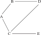
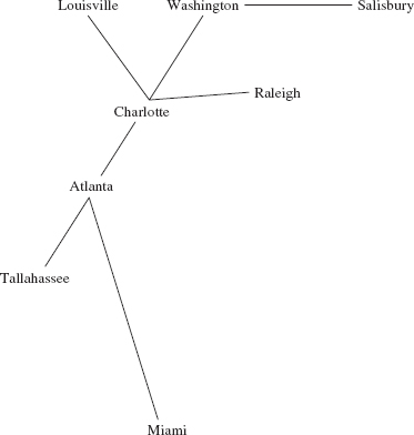
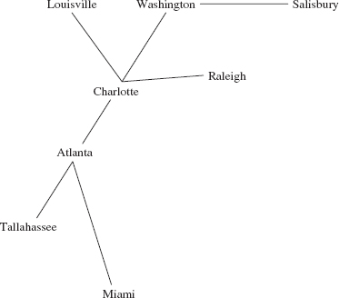
Figure 15.2a contains several additional undirected graphs. Notice that the number of edges can be fewer than the number of vertices (Figures 15.2a and b), equal to the number of vertices (Figure 15.1) or greater than the number of vertices (Figure 15.2c).
FIGURE 15.2a An undirected graph with six vertices and five edges
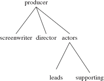
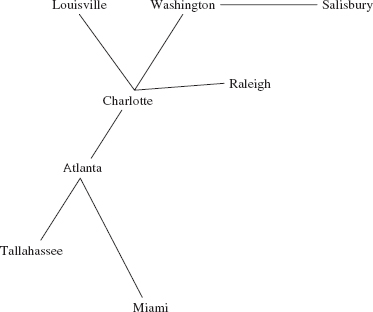
FIGURE 15.2b An undirected graph with eight vertices and seven edges

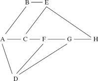
FIGURE 15.2c An undirected graph with eight vertices and eleven edges
An undirected graph is complete if it has as many edges as possible. What is the number of edges in a complete undirected graph? Let n represent the number of vertices. Figure 15.3 shows that when n = 6, the maximum number of edges is 15.
FIGURE 15.3 An undirected graph with 6 vertices and the maximum number (15) of edges for any undirected graph with 6 vertices
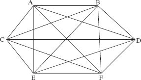
Can you determine a formula that holds for any positive integer n? In general, start with any one of the n vertices, and construct an edge to each of the remaining n – 1 vertices. Then from any one of those n – 1 vertices, construct an edge to each of the remaining n – 2 vertices (the edge to the first vertex was constructed in the previous step). Then from any one of those n – 2 vertices, construct an edge to each of the remaining n – 3 vertices. This process continues until, at step n – 1, a final edge is constructed. The total number of edges constructed is:
This last equality can either be proved directly by induction on n or can be derived from the proof—in Example A2.1 of Appendix 2—that the sum of the first n positive integers is equal to n (n + 1)/2.
Two vertices are adjacent if they form an edge. For example, in Figure 15.2b, Charlotte and Atlanta are adjacent, but Atlanta and Raleigh are not adjacent. Adjacent vertices are called neighbors.
A path is a sequence of vertices in which each successive pair is an edge. For example, in Figure 15.2c,
A, B, E, H
is a path from A to H because (A, B), (B, E), and (E, H) are edges. Another path from A to H is
A, C, F, D, G, H
For a path of k vertices, the length of the path is k – 1. In other words, the path length is the number of edges in the path. For example, in Figure 15.2c the following path from C to A has a length of 3:
C, F, D, A
There is, in fact, a path with fewer edges from C to A, namely,
C, A
In general, there may be several paths with fewest edges between two vertices. For example, in Figure 15.2c,
A, B, E
and
A, C, E
are both paths with fewest edges from A to E.
A cycle is a path in which the first and last vertices are the same and there are no repeated edges. For example, in Figure 15.1,
A, B, D, C, A
is a cycle. In Figure 15.2c,
B, E, H, G, D, A, B
is a cycle, as is
E, C, A, B, E
The undirected graph in Figures 15.2a and b are acyclic, that is, they do not contain any cycles. In Figure 15.2a,
producer, director, producer
is not a cycle since the edge (producer, director) is repeated—recall that an edge in an undirected graph is an unordered pair.
An undirected graph is connected if, for any given vertex, there is a path from that vertex to any other vertex in the graph. Informally, an undirected graph is connected if it is "all one piece." For example, all of the graphs in the previous figures are connected. The following undirected graph, with six vertices and five edges, is not connected:

15.2 Directed Graphs
Up to now we have not concerned ourselves with the direction of edges. If we could go from vertex V to vertex W, we could also go from vertex W to vertex V. In many situations this assumption may be unrealistic. For example suppose the edges represent streets and the vertices represent intersections. If the street connecting vertex V to vertex W is one-way going from V to W, there would be no edge connecting W to V.
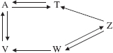
A directed graph—sometimes called a digraph—is a collection of vertices and edges in which the edges are ordered pairs of vertices. For example, here is a directed graph, with edges in angle brackets to indicate an ordered pair:
Vertices:A, T, V, W, Z
Edges: (A, T), (A, V), (T, A), (V, A), (V, W), (W, Z), (Z, W>, (Z, T)
Pictorially, these edges are represented by arrows, with the arrow's direction going from the first vertex in the ordered pair to the second vertex. For example, Figure 15.4 contains the directed graph just defined.
A path in a directed graph must follow the direction of the arrows. Formally a path in a directed graph is a sequence of k > 1 vertices V0, V1,..., Vk-1 such that (V0, V1), (V1, V2),..., (Vk-2, Vk-1) are edges in the directed graph. For example, in Figure 15.4,
A, V, W, Z
is a path from A to Z because (A, V), (V, W), and (W, Z) are edges in the directed graph. But
A, T, Z, W
is not a path because there is no edge from T to Z, (In other words, Z is not a neighbor of T, although T is a neighbor of Z.) A few minutes checking should convince you that for any two vertices in Figure 15.4, there is a path from the first vertex to the second.
Adigraph D isconnected if, for any pair of distinct vertices x and y, there is a path from x to y. Figure 15.4 is a connected digraph, but the digraph in Figure 15.5 is not connected (try to figure out why):
From these examples, you can see that we actually could have defined the term "undirected graph" from "directed graph": an undirected graph is a directed graph in which, for any two vertices V and W,

FIGURE 15.5 A digraph that is not connected
if there is an edge from V to W, there is also an edge from W to V. This observation will come in handy when we get to developing Java classes.
In the next two sections, we will look at specializations of graphs: trees and networks.
15.3 Trees
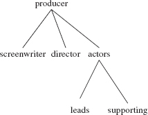
An undirected tree is a connected, acyclic, undirected graph with one element designated as the root element. Note that any element in the graph can be designated as the root element. For example, here is the undirected tree from Figure 15.2a; producer is designated as the root element.
On most occasions, we are interested in directed trees, that is, trees that have arrows from a parent to its children. A tree, sometimes called a directed tree, is a directed graph that either is empty or has an element, called the root element such that:
- there are no edges coming into the root element;
- every non-root element has exactly one edge coming into it;
- there is a path from the root to every other element.
For example, Figure 15.6 shows that we can easily re-draw the undirected tree as a directed tree:
Many of the binary-tree terms from Chapter 9—such as "child", "leaf", "branch"—can be extended to apply to arbitrary trees. For example, the tree in Figure 15.6 has four leaves and height 2. But "full" does not apply to trees in general because there is no limit to the number of children a parent can have. In fact, we cannot simply define a binary tree to be a tree in which each element has at most two children. Why not? Figure 15.7 has two distinct binary trees that are equivalent as trees.
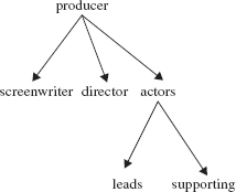
FIGURE 15.7 Two distinct binary trees, one with an empty right subtree and one with an empty left subtree
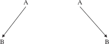
We can define a binary tree to be a (directed) tree in which each vertex has at most two children, labeled the "left" child and the "right" child of that vertex.
Trees allow us to study hierarchical relationships such as parent-child and supervisor-supervisee. With arbitrary trees, we are not subject to the at-most-two-children restriction of binary trees.
15.4 Networks
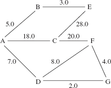
Sometimes we associate a non-negative number with each edge in a graph (which can be directed or undirected). The non-negative numbers are called weights, and the resulting structure is called a weighted graph or network. For example, Figure 15.8 has an undirected network in which each weight represents the distance between cities for the graph of Figure 15.2b.
Of what value is a weighted digraph, that is, why might the direction of a weighted edge be significant? Even if one can travel in either direction on an edge, the weight for going in one direction may be different from the weight going in the other direction. For example, suppose the weights represent the time for a plane flight between two cities. Due to the prevailing westerly winds, the time to fly from New York to Los Angeles is usually longer than the time to fly from Los Angeles to New York.
FIGURE 15.8 An undirected network in which vertices represent cities, and each edge's weight represents the distance between the two cities in the edge
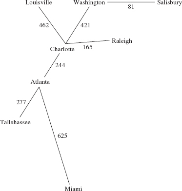
FIGURE 15.9 A weighted digraph with 8 vertices and 11 edges

Figure 15.9 shows a weighted digraph in which the weight of the edge from vertex D to vertex F is different from the weight of the edge going in the other direction.
With each path between two vertices in a network, we can calculate the total weight of the path. For example, in Figure 15.9, the path A, C, D, E has a total weight of 10.0. Can you find a shorter path from A to E, that is, a path with smaller total weight1? The shortest path from A to E is A, B, D, E with total weight 8.0. Later in this chapter we will develop an algorithm to find a shortest path (there may be several of them) between two vertices in a network.
The weighted digraph in Figure 15.9 is not connected because, for example, there is no path from B to C. Recall that a path in a digraph must follow the direction of the arrows.
Now that we have seen how to define a graph or tree (directed or undirected, weighted or unweighted), we can outline some well-known algorithms. The implementation of those algorithms, and their analysis, will be handled in Section 15.6.3.
15.5 Graph Algorithms
A prerequisite to other graph algorithms is being able to iterate through a graph, so we start by looking at iterators in general. We focus on two kinds of iterators: breadth-first and depth-first. These terms may ring a bell; in Chapter 9, we studied breadth-first and depth-first (also known as pre-order) traversals of a binary tree.
15.5.1 Iterators
There are several kinds of iterators associated with directed or undirected graphs, and these iterators can also be applied to trees and networks (directed or undirected). First, we can simply iterate over all of the vertices in the graph. The iteration need not be in any particular order. For example, here is an iteration over the vertices in the weighted digraph of Figure 15.9:
A, B, D, F, G, C, E, H
In addition to iterating over all of the vertices in a graph, we are sometimes interested in iterating over all vertices reachable from a given vertex. For example, in the weighted digraph of Figure 15.9, we might want to iterate over all vertices reachable from A, that is, over all vertices that are in some path that starts at A. Here is one such iteration:
A, B, C, D, E, F, H
The vertex G is not reachable from A, so G will not be in any iteration from A.
15.5.1.1 Breadth-First Iterators
A breadth-first iterator, similar to a breadth-first traversal in Chapter 9, visits vertices in order, beginning with some vertex identified as the "start vertex." What is the order? Roughly, it can be described as "neighbors first." As soon as a vertex has been visited, each neighbor of that vertex is marked as "reachable," and vertices are visited in the order in which they are marked as reachable. The first vertex marked as reachable and visited is the start vertex, then the neighbors of the start vertex are marked as reachable, so they are visited, then the neighbors of those neighbors, and so on.
No vertex is visited more than once, and any vertex that is not on some path from the start vertex will not be visited at all. For example, assume that the vertices in the following graph—from Figure 15.2b—were entered in alphabetical order:
We will perform a breadth-first iteration starting at Atlanta and visit neighbors in alphabetical order. So we start with
r, v
Atlanta
The r and v above Atlanta indicate that Atlanta has been marked as reachable and visited. The neighbors of Atlanta are now marked as reachable:
r,v r r r
Atlanta, Charlotte, Miami, Tallahassee
Each of those neighbors of Atlanta is then visited in turn, and when a city is visited, each of its neighbors is marked as reachable—unless that neighbor was marked as reachable previously. When we visit Charlotte, we have
r,v r,v r r r r r
Atlanta, Charlotte, Miami, Tallahassee, Louisville, Raleigh, Washington
Notice that the first neighbor of Charlotte, Atlanta, is ignored because we have already marked as reachable (and visited) Atlanta. Then Miami is visited (its only neighbor has already been marked as reachable), Tallahassee (its only neighbor has already been marked as reachable), Louisville (its only neighbor has already been marked as reachable), Raleigh (its only neighbor has already been marked as reachable), and Washington, whose neighbor Salisbury is now marked as reachable. We now have
r,v r,v r,v r,v r,v r,v r,v r
Atlanta, Charlotte, Miami, Tallahassee, Louisville, Raleigh, Washington Salisbury
When we visit Salisbury we are done because Salisbury has no not-yet-reached neighbors marked as not reachable. In other words, we have iterated through all cities reachable from Atlanta, starting at Atlanta:
Atlanta, Charlotte, Miami, Tallahassee, Louisville, Raleigh, Washington, Salisbury
The order of visiting cities would be different if we started a breadth-first iteration at Louisville:
Louisville, Charlotte, Atlanta, Raleigh, Washington, Miami, Tallahassee, Salisbury
Let's do some preliminary work on the design of the BreadthFirstiterator class. When a vertex has been marked as reachable, that vertex will, eventually, be visited. To make sure that vertex is not re-visited, we will keep track of which vertices have already been marked as reachable. To do this, we will store the marked-as-reachable vertices in some kind of collection. Specifically, we want to visit the neighbors of the current vertex in the order in which those neighbors were initially stored in the collection. Because we want the vertices removed from the collection in the order in which they were added to the collection, a queue is the appropriate collection. And we will also want to keep track of the current vertex.
We can now develop high-level algorithms for the BreadthFirstiterator methods—the details will have to be postponed until we create a class—such as Network, in which BreadthFirstiterator will be embedded. The constructor enqueues the start vertex and marks all other vertices as not reachable:
public BreadthFirstIterator (Vertex start)
{
     for every vertex in the graph:
            mark that vertex as not reachable.
     mark start as reachable.
     queue.enqueue (start);
} // algorithm for constructor
The hasNext() method returns !queue.isEmpty(). The next() method removes the front vertex from the queue, makes that vertex the current vertex, and enqueues each neighbor of the current vertex that has not yet been marked as reachable:
public Vertex next()
{
       current = queue.dequeue();

for each vertex that is a neighbor of current:
             if that vertex has not yet been marked as reachable
             {
                   mark that vertex as reachable;
                   enqueue that vertex;
             } // if
       return current;
} // algorithm for method next
The analysis of this algorithm is postponed until Section 15.6.3, when we will have all of the details associated with the BreadthFirstIterator class.
The remove() method deletes from the graph the current vertex, that is, the vertex most recently returned by a call to the next() method. All edges going into or out of that current vertex are also deleted from the graph.
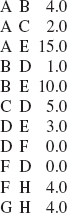
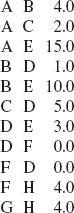
For an example of how the queue and the next() method work together in a breadth-first iteration, suppose we create a weighted digraph by entering the sequence of edges and weights in Figure 15.10.
FIGURE 15.10 A sequence of edges and weights to generate the weighted digraph in Figure 15.9
The weighted digraph created is the same one shown in Figure 15.9:

To conduct a breadth-first iteration starting at A, for example, we first enqueue A in the constructor. The first call to next() dequeues A, enqueues B, C and E, and returns A. The second call to next() dequeues B, enqueues D, and returns B. Figure 15.11 shows the entire queue generated by a breadth-first iteration starting at A.
FIGURE 15.11 A breadth-first iteration of the vertices starting at A. The vertices are enqueued—and therefore dequeued—in the same order in which they were entered in Figure 15.10
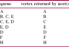
Notice that vertex G is missing from Figure 15.11. The reason is that G is not reachable from A, that is, there is no path from A to G. If we performed a breadth-first iteration from any other vertex, there would be even fewer vertices visited than in Figure 15.11. For example, a breadth-first iteration starting at vertex B would visit
B, D, E, F, H
in that order.
Breadth-first iterators are especially useful in iterating over a (directed) tree. The start vertex is the root and, as we saw in Chapter 9, the vertices are visited level-by-level: the root, the root's children, the root's grandchildren, and so on.
15.5.1.2 Depth-First Iterators
The other specialized iterator is a depth-first iterator. A depth-first iterator is a generalization of the pre-order traversal of Chapter 9. To refresh your memory, here is the algorithm for a pre-order traversal of a binary tree t:
preOrder (t)
{
     if (t is not empty)
     {
             access the root element of t;
             preOrder (leftTree (t));
             preOrder (rightTree (t));
     } // if
} // preOrder traversal
To further help you recall how a pre-order traversal works, Figure 15.12 shows a binary tree and a pre-order traversal of its elements.
We can describe a pre-order traversal of a binary tree as follows: start with a leftward path from the root. Once the end of a path is reached, the algorithm backtracks to an element that has an as-yet-unreachable right child. Another leftward path is begun, starting with that right child.
A depth-first iteration of a graph proceeds similarly to a breadth-first iteration. We first mark as not reachable each vertex, then mark as reachable, and visit, the start vertex. Then we mark as reachable each neighbor of the start vertex. Next, we visit the most recently marked as reachable vertex of those neighbors, and mark as reachable each not-yet-marked-as-reachable neighbor of that vertex. Another path is begun starting with that unvisited vertex. This continues as long as there are vertices reachable from the start vertex that have not yet been found to be reachable.
FIGURE 15.12 A binary tree and the order in which its elements would be visited during a pre-order traversal

For example, let's perform a depth-first iteration of the following graph, starting at Atlanta—we assume that the vertices were initially entered in alphabetical order:
We first visit the start vertex:
r, v
Atlanta
Then we mark as reachable the neighbors of Atlanta:
r,v r r r
Atlanta, Charlotte, Miami, Tallahassee
We then visit the most recently marked as reachable vertex, namely Tennessee, not Charlotte. Tallahassee's only neighbor has already been marked as reachable, so we visit the next-most-recently marked-as-reachable vertex: Miami. Miami's only neighbor has already been marked as reachable, so we visit Charlotte, and mark as reachable Louisville, Raleigh and Washington, in that order. We now have
r,v r,v r,v r,v r r r
Atlanta, Charlotte, Miami, Tallahassee, Louisville, Raleigh, Washington
Washington, the most recently marked-as-reachable vertex, is visited, and its only not yet marked-as-reachable neighbor, Salisbury, is marked as reachable. We now have
r,v r,v r,v r,v r r r,v r
Atlanta, Charlotte, Miami, Tallahassee, Louisville, Raleigh, Washington Salisbury
Now Salisbury is the most recently marked-as-reachable vertex, so Salisbury is visited. Finally, Raleigh and then Louisville are visited. The order in which vertices are visited is as follows:
Atlanta, Tallahassee, Miami, Charlotte, Washington, Salisbury, Raleigh, Louisville
For a depth-first iteration starting at Charlotte, the order in which vertices are visited is:
Charlotte, Washington, Salisbury, Raleigh, Louisville, Atlanta, Tallahassee, Miami
With a breadth-first iteration, we saved vertices in a queue so that the vertices were visited in the order in which they were saved. With a depth-first iteration, the next vertex to be visited is the most recently reached vertex. So the vertices will be stacked instead of queued. Other than that, the basic strategy of a depth-first iterator is exactly the same as the basic strategy of a breadth-first iterator. Here is the high-level algorithm for next():
public Vertex next()
{
       current = stack.pop();


       for each vertex that is a neighbor of current:
             if that vertex has not yet been marked as reachable
             {
                   mark that vertex as reachable;
                   push that vertex onto stack;
             } // if
       return current;
} // algorithm for method next
The analysis of this algorithm is the same as that of the next() method in the BreadthFirstIterator class: see Section 15.6.3.
Suppose, as we did above, we create a weighted digraph from the following input, in the order given:
The weighted digraph created is the same one shown in Figure 15.9:
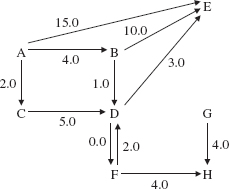
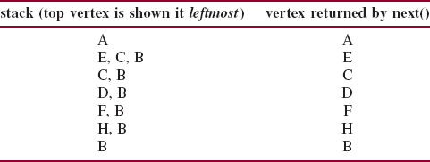
Figure 15.13 shows the sequence of stack states and the vertices returned by next() for a depth-first iteration of the weighted digraph in Figure 15.9, as generated from the input in Figure 15.10.
We could have developed a backtrack version of the next() method. The vertices would be visited in the same order, but recursion would be utilized instead of an explicit stack.
When should you use a breadth-first iterator and when should you use a depth-first iterator? If you are looping through all vertices reachable from the start vertex, there's not much reason to pick. The only difference is the order in which the vertices will be visited. But if you are at some start vertex and you are searching for a specific vertex reachable from that start vertex, there can be a difference. If, somehow, you know that there is a short path from the start vertex to the vertex sought, a breadth-first iterator is preferable: the vertices on a path of length 1 from the start vertex are visited, then the vertices on a path of length 2, and so on. On the other hand, if you know that the vertex sought may be very far from the start vertex, a depth-first search will probably be quicker (see Figure 15.12).
FIGURE 15.13 A depth-first iteration of the vertices reachable from A. We assume the vertices were entered as in Figure 15.10
15.5.2 Connectedness
In Section 15.1, we defined an undirected graph to be connected if, for any given vertex, there is a path from that vertex to any other vertex in the graph. For example, the following is a connected, undirected graph:
For a digraph, that is, a directed graph, connectedness means that for any two distinct vertices, there is a path—that follows the directions of the arrows—between them. A breadth-first or depth-first iteration over all vertices in a graph can be performed only if the graph is connected. In fact, we can use the ability to iterate between any two vertices as a test for connectedness of a digraph.
Given a digraph, let itr be an iterator over the digraph. For each vertex v returned by itr.next(), let bfitr be a breadth-first iterator starting at v. We check to make sure that the number of vertices reachable from v (including v itself) is equal to the number of vertices in the digraph.
Here is a high-level algorithm to determine connectedness in a digraph:
public boolean isConnected()
{
    for each Vertex v in this digraph
    {
      // Count the number of vertices reachable from v.
      Construct a BreadthFirstIterator, bfItr, starting at v.
      int count = 0;
      while (bfItr.hasNext())

      {
             bfItr.next();
             count++;
      } // while
      if (count < number of vertices in this digraph)
        return false;
    } // for
    return true;
} // algorithm for isConnected
For an undirected graph, the isConnected() algorithm is somewhat simpler: there is no need for an outer loop to iterate through the entire graph. See Concept Exercise 15.4.
In the next two sections, we outline the development of two important network algorithms. Each algorithm is sufficiently complex that it is named after the person (Prim, Dijkstra) who invented the algorithm.
15.5.3 Generating a Minimum Spanning Tree
Suppose a cable company has to connect a number of houses in a community. Given the costs, in hundreds of dollars, to lay cable between the houses, determine the minimum cost of connecting the houses to the cable system. This can be cast as a connected network problem; each weight represents the cost to lay cable between two neighbors. Figure 15.14 gives a sample layout. Some house-to-house distances are not given because they represent infeasible connections (over a mountain, for example).
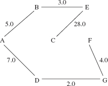
In a connected, undirected network, a spanning tree is a weighted tree that consists of all of the vertices and some of the edges (and their weights) from the network. Because a tree must be connected, a spanning tree connects all of the vertices of the original graph. For example, Figures 15.15 and 15.16 show two spanning trees for the network in Figure 15.14. For the sake of specificity, we designate vertex A as the root of each tree, but any other vertex would serve equally well.
A minimum spanning tree is a spanning tree in which the sum of all the weights is no greater than the sum of all the weights in any other spanning tree. The original problem about laying cable can be re-stated in the form of constructing a minimum spanning tree for a connected network. To give you an idea of how difficult it is to solve this problem, try to construct a minimum spanning tree for the network in Figure 15.14. How difficult would it be to "scale up" your solution to a community with 1,000 houses?
FIGURE 15.14 A connected network in which the vertices represent houses and the weights represent the cost, in hundreds of dollars, to connect the two houses
An algorithm to construct a minimum spanning tree is due to R. C. Prim [1957]. Here is the basic strategy. Start with an empty tree T and pick any vertex v in the network. Add v to T. For each vertex w such that (v, w) is an edge with weight wweight, save the ordered triple (v, w, wweight} in a collection—we'll see what kind of collection shortly. Then loop until T has as many vertices as the original network. During each loop iteration, remove from the collection the triple (x, y, yweight} for which yweight is the smallest weight of all triples in the collection; if y is not already in T, add y and the edge (x, y) to T and save in the collection every triple (y, z, zweight} such that z is not already in T and (y, z) is an edge with weight zweight.
FIGURE 15.15 A spanning tree for the network in Figure 15.14
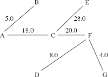
FIGURE 15.16 Another spanning tree for the network in Figure 15.14
What kind of collection should we have? The collection should be ordered by weights; we need to be able to add an element, that is, a triple, to the collection and to remove the triple with lowest weight. A priority queue will perform these tasks quickly. Recall from Chapter 13 that for the PriorityQueue class, averageTime(n) for the add (E element) method is constant, and averageTime(n) for the remove() method is logarithmic in n.
To see how Prim's algorithm works, let's start with the network in Figure 15.14, repeated here:

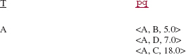
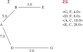
Initially, the tree T and the priority queue pq are both empty. Add A to T, and add to pq each triple of the form (A, w, wweight} where (A, w) is an edge with weight wweight. Figure 15.17 shows the contents of T and pq at this point. For the sake of readability, the triples in pq are shown in increasing order of weights; strictly speaking, all we know for sure is that the element() and remove() methods return the triple with smallest weight.
FIGURE 15.17 The contents of T and pq at the start of Prim's algorithm as applied to the network in Figure 15.14
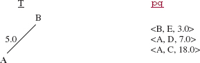
When the lowest-weighted triple, (A, B, 5.0) is removed from pq, the vertex B and the edge (A, B) are added to T, and the triple (B, E, 3.0) is added to pq. See Figure 15.18.
FIGURE 15.18 The contents of T and pq during the application of Prim's algorithm to the network in Figure 15.14
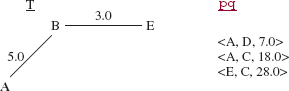
During the next iteration, the triple (B, E, 3.0) is removed from pq, the vertex E and edge (B, E) are added to T, and the triple (E, C, 28.0) is added to pq. See Figure 15.19.
FIGURE 15.19 The contents of T and pq during the application of Prim's algorithm to the network in Figure 15.14
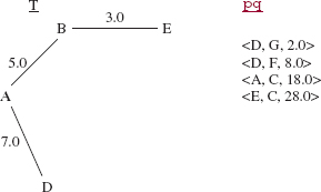
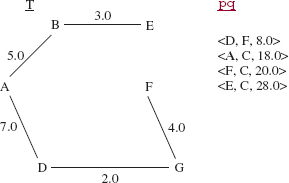
During the next iteration, the triple (A, D, 7.0) is removed from pq, the vertex D and the edge (A, D) are added to T, and the triples (D, F, 8.0) and (D, G, 2.0) are added to pq. See Figure 15.20.
FIGURE 15.20 The contents of T and pq during the application of Prim's algorithm to the network in Figure 15.14
During the next iteration, the triple (D, G, 2.0} is removed from pq, the vertex G and the edge (D, G) are added to T, and the triple (G, F, 4.0} is added to pq. See Figure 15.21.
FIGURE 15.21 The contents of T and pq during the application of Prim's algorithm to the network in Figure 15.14
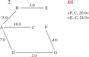
During the next iteration, the triple (G, F, 4.0} is removed from pq, the vertex F and the edge (G, F) are added to T, and the triple (F, C, 20.0} is added to pq. See Figure 15.22.
FIGURE 15.22 The contents of T and pq during the application of Prim's algorithm to the network in Figure 15.14
During the next iteration, the triple (D, F, 8.0} is removed from pq. But nothing is added to T or pq because F is already in T!
During the next iteration, the triple (A, C, 18.0} is removed from pq, the vertex C and the edge (A, C) are added to T, and nothing is added to pq. The reason nothing is added to pq is that, for all of C's edges, (C, A), (C, E) and (C, F), the second element in the pair is already in T. See Figure 15.23.
Even though pq is not empty, we are finished because every vertex in the original network is also in T.
From the way T is constructed, we know that T is a spanning tree. We can show, by contradiction, that T is a minimum spanning tree. In general, a proof by contradiction assumes some statement to be false, and shows that some other statement—known to be true—must also be false. We then conclude that the original statement must have been true.
FIGURE 15.23 The contents of T and pq after the last iteration in the application of Prim's algorithm to the network in Figure 15.14
Assume that T is not a minimum spanning tree. Then during some iteration, a triple ( x, y, yweight) is removed from pq and the edge (x, y) is added to T, but there is some vertex v, already in T, and w, not in T, such that edge (v, w) has lower weight than edge (x, y). Pictorially:
Note that since v is already in T, the triple starting with (v, w, ?) must have been added to pq earlier. But the edge (v, w) could not have a lower weight than the edge (x, y) because the triple (x, y, y weight) was removed from pq, not the triple starting with (v, w, ?). This contradicts the claim that (v, w) had lower edge weight than (x, y). So T, with edge (x, y) added, must still be minimum.
Can Prim's algorithm be applied to a connected, directed network? Consider the following network: (<a, b, 8.0>, <b, c, 5.0>, <c, a, 10.0>). Prim's algorithm would give a different result depending on which vertex was chosen as the root. We can—and will—apply Prim's algorithm to a connected directed network provided it is equivalent to its undirected counterpart. That is, for any pair of vertices u and v, if v is a neighbor of u then u is a neighbor of v, and the weights of the two edges are the same.
Prim's algorithm is another example of the greedy-algorithm design pattern (the Huffman encoding algorithm in Chapter 13 is also a greedy algorithm). During each loop iteration, the locally optimal choice is made: the edge with lowest weight is added to T. This sequence of locally optimal—that is, greedy—choices leads to a globally optimal solution: T is a minimum spanning tree.
Another greedy algorithm appears in Section 15.5.4. Concept Exercise 15.7 and Lab 23 show that greed does not always succeed.
15.5.4 Finding the Shortest Path through a Network
In Section 15.4.3, we developed a strategy for constructing a minimum spanning tree in a network. A similar strategy applies to finding a shortest path in a network (directed or undirected) from some vertex v1 to some other vertex v2. In this context, "shortest" means having the lowest total weight. Both algorithms are greedy, and both use a priority queue. The shortest-path algorithm, due to Edsgar Dijkstra [1959], is essentially a breadth-first iteration that starts at v1 and stops as soon as v2's pair is removed from the priority queue pq. (Dijkstra's algorithm actually finds a shortest path from v1 to every other vertex in the network.) Each pair consists of a vertex w and the sum of the weights of all edges on the shortest path so far from v1 to w.
The priority queue is ordered by lowest total weights. To keep track of total weights, we have a map, weightSum, in which each key is a vertex w and each value is the sum of the weights of all the edges on the shortest path so far from v1 to w. To enable us to re-construct the shortest path when we are through, there is another map, predecessor, in which each key is a vertex w, and each value is the vertex that is the immediate predecessor of w on the shortest path so far from v1 to w.
Basically, weightSum maps each given vertex to the minimum total weight, so far, of the path from v1 to the given vertex. Initially, pq consists of vertex v1 and its weight, 0.0. On each iteration we greedily choose the vertex-weight pair (x, total weight} in pq that has the minimum total weight among all vertex-weight pairs in pq. If there is a neighbor y of x whose total weight can be reduced by the path (v1,..., x, y}, then y's path and minimum weight are altered, and y (and its new total weight) is added to pq. For example, we might have the partial network shown in Figure 15.24.
FIGURE 15.24 The minimum-weight path from vertex v1 to vertex y had been 15, but the path from vertex v1 through vertex x to vertex y has a lower total weight
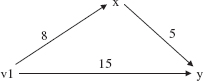
Then the total weight between v1 and y is reduced to 13, the pair (y, 13} is added to pq and y's predecessor becomes x. Eventually, this yields the shortest path from v1 to v2, if there is a path between those vertices.
To start, weightSum associates with each vertex a very large total weight, and predecessor associates with each vertex the value null. We then refine those initializations by mapping v1's weightSum to 0, mapping v1's predecessor to v1 itself, and adding (v1, 0.0) to pq. This completes the initialization phase.
Suppose we want to find the shortest path from A to E in the network from Figure 15.9, repeated here:

For simplicity, we ignore G because, in fact, G is not reachable from A. Initially, we have
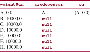
After initializing, we keep looping until E is removed from pq (that is, until the shortest path is found) or pq is empty (that is, there is no path from A to E). During the first iteration of this loop, the minimum (and only) pair, (A, 0.0), is removed from pq. Since that pair's weight, 0.0, is less than or equal to A's weightSum value, we iterate, in an inner loop, over the neighbors of A. For each neighbor of A, if A's weightSum value plus that neighbor's weight is less than the neighbor's weightSum value, weightSum, and predecessor are updated, and the neighbor and its total weight (so far) are added to pq. The effects are shown in Figure 15.25.
FIGURE 15.25 Dijkstra's shortest-path algorithm, after the first iteration of the outer loop
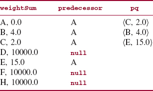
After the processing shown in Figure 15.25, the outer loop is executed for a second time: the pair (C, 2.0) is removed from pq and we iterate (the inner loop) over the neighbors of C. The only vertex on an edge from C is D, and the weight of that edge is 5.0. This weight plus 2.0 (C's weight sum) is 7.0, which is less than D's weight sum, 10000.0). So in weightSum, D's weight sum is upgraded to 7.0. Figure 15.26 shows the effect on weightSum, predecessor, and pq.
Figure 15.26 indicates that at this point, the lowest-weight path from A to D has a total weight of 7.0. During the third iteration of the outer loop, (B, 4.0) is removed from pq and we iterate over the neighbors of B, namely, D and E. The effects are shown in Figure 15.27.
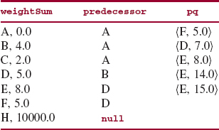
At this point, the lowest-weight path to D has a total weight of 5.0 and the lowest-weight path to E has a total weight of 14.0. During the fourth iteration of the outer loop, (D, 5.0) is removed from pq, and we iterate over the neighbors of D, namely, F and E. Figure 15.28 shows the effects of this iteration.
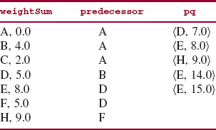
During the fifth outer-loop iteration, (F, 5.0) is removed from pq, the neighbors of F, namely D and H are examined, and the collections are updated. See Figure 15.29.
FIGURE 15.26 The state of the application of Dijkstra's shortest-path algorithm after the second iteration of the outer loop
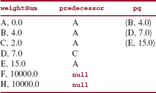
FIGURE 15.27 The state of the application of Dijkstra's shortest-path algorithm after the third iteration of the outer loop
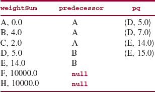
FIGURE 15.28 The state of the application of Dijkstra's shortest-path algorithm after the fourth iteration of the outer loop
During the sixth iteration of the outer loop, (D, 7.0} is removed from pq. The minimum total weight, so far, from A to D is recorded in weightSum as 5.0. So there is no inner-loop iteration.
During the seventh iteration of the outer loop, (E, 8.0} is removed from pq. Because E is the vertex we want to find the shortest path to, we are done. How can we be sure there are no shorter paths to E? If there were another path to E with total weight t less than 8.0, then the pair (E, t} would have been removed from pq before the pair (E, 8.0}.
FIGURE 15.29 The state of the application of Dijkstra's shortest-path algorithm after the fifth iteration of the outer loop
We construct the shortest path, as a LinkedList of vertices, from predecessor: starting with an empty LinkedList object, we prepend E; then prepend D, the predecessor of E; then prepend B, the predecessor of D; finally, prepend A, the predecessor of B. The final contents of the LinkedList object are, in order,
A, B, D, E
There are a few details that are missing in the above description of Dijkstra's algorithm. For example, how will the vertices, edges, and neighbors be stored? What are worstTime(n) and averageTime(n)?To answer these questions, we will develop a class in Section 15.6.3, and fill in the missing details, not only of Dijkstra's algorithm, but of all our graph-related work.
15.5.5 Finding the Longest Path through a Network?
Interestingly, it is often important to be able to find a longest path through a network. A project network is an acyclic, directed network with a single source (no arrows coming into it) and a single sink (no arrows going out from it). The source and sink are usually labeled S (for start) and T (for terminus), respectively. Figure 15.30 shows a project network.
We can interpret the edges in a project network as activities to be performed, the weights as the time in days (or cost in dollars) required for the activities, and the vertices as events that indicate the completion of all activities coming into the event. With that interpretation, the project length, that is, the length of a longest path, represents the number of days required to complete the project. For example, in Figure 15.30, there are two longest paths:
FIGURE 15.30 A project network
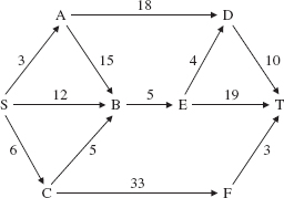
S, A, B, E, T
and
S, C, F, T
Each of those paths has a length of 42, so the project, as scheduled, will take 42 days. Dijkstra's algorithm can easily be modified to find a longest path in an acyclic network. The next section, on topological sorting, can be used to determine if a network is acyclic.
In a project network, some activities can occur concurrently, and some activities can be delayed without affecting the project length. A project manager may want to know which activities can be delayed without delaying the entire project. First, we need to make some calculations.
For each event w, we can calculate ET(w), the earliest time that event w can be completed. For event S, ET(S) is 0. For any other event w, ET(w) is the maximum of {ET(v) + weight (v, w)} for any event v such that (v, w} forms an edge. For example, in Figure 15.30, ET(C) = 6, ET (B) = max {12, 18, 11}= 18, ET(E) = 23, ET (D) = max {21, 27} = 27, and so on.
For each event w, we can also calculate LT(w), the latest time by which w must be completed to avoid delaying the entire project. For event T, LT(T) is the project length; for any other event w, LT(w) is the minimum of {LT(x) – weight(w, x)} for any event x such that (w, x} forms an edge. For example, in Figure 15.30, LT(T) = 42, LT(D) = 32, LT(E) = min {28, 23} = 23, LT(B) = 18, LT (C) = min {6, 13}=6, and so on.
Finally, ST(y, z), the slack time of activity (y, z}, is calculated as follows:
ST(y, z) = LT(z) − ET(y) − weight(y, z)
For example, in Figure 15.30,
ST(S, C) = LT(C) − ET(S) − weight(S, C) = 6 − 0 − 6 = 0
ST(A, B) = LT(B) − ET(A) − weight(A, B) = 18−3 −15 = 0
ST(A, D) = LT(D) − ET(A) −weight(A, D) = 32 −3 −18= 11
An activity with a slack time of zero is called a critical activity, and any path that consists only of critical activities is called a critical path. The idea is that special attention should be given to any critical activity because any delay in that activity will increase the project length.
Activities that are not on a critical path are less constrained: They may be delayed or take longer than scheduled without affecting the length of the entire project. For example, in Figure 15.30, the activity ( A, D} has a slack time of 11 days: That activity can be delayed or take longer than scheduled, as long as the activity is completed by day 32. The significance of this is that resources allocated to activity (A, D} can be diverted to a critical task, and thereby speed up the completion of the entire project.
Programming Project 15.3 entails finding the slack time for each project in a project network. In order to calculate the earliest times for each event, the events must be ordered so that for example, when ET(w) is to be calculated for some vertex w, the value of ET(v) must already be available for each vertex v such that (v, w} forms an edge. Section 15.5.5.1 describes that kind of ordering.
15.5.5.1 Topological Sorting
A network with a cycle cannot have a longest path because we could continuously loop through the cycle to create a path whose total weight is arbitrarily large. We will soon see how to determine if a network is acyclic.
The calculation of earliest times and latest times for the project network in Section 15.5.5 requires that the events be in order. Specifically, to calculate ET(w) for some vertex w, we need to know ET(v), for any vertex v such that ( v, w) forms an edge. If the project network is small and the calculations are being done by hand, this ordering can be made implicitly. But for a large project, or for a program to perform the calculations, the ordering must be explicit. To calculate LT(w) for any vertex w, the reverse of this ordering is needed.
The ordering is not, necessarily, the one provided by a breadth-first iterator, a depth-first iterator, or an iterator over the entire network. The ordering is called a "topological ordering." The vertices v1, v2,... of a digraph are in topological order if vi precedes vj in the ordering whenever ( vi, vj) forms an edge in the digraph. The arranging of vertices into a topological ordering is called topological sorting. For example, for the digraph in Figure 15.30, here is a topological order:
S, A, C, B, E, F, D, T
Notice that D had to come after both A and E because (A, D) and (E, D) are edges in the digraph. Another topological order is
S, A, C, F, B, E, D, T
Any network that can be put into topological order must be acyclic. Concept Exercise 15.12 has more information about topological order, and Programming Exercise 15.5 suggests how to perform a topological sort.
15.6 A Network Class
In this chapter, we have introduced eight different data types: a graph and a tree, each of which can be directed or undirected, and weighted or unweighted. We would like to develop classes for these collections with a maximum amount of code sharing. The object-oriented solution is to utilize inheritance, but exactly how should this be done? If we make the Digraph class a subclass of UndirectedGraph, then virtually all of the code relating to edges will have to be overridden. That's because in an undirected graph, each edge A, B represents two links: from A to B and from B to A. Similarly, code written for graphs would have to be re-written for networks.
A better approach is to define the (directed) Network class, and make the other classes subclasses of that class. For example, we can view an undirected network as a directed network in which all edges are two-way. So to add an edge A, B in an undirected network, the method definition is:
/**
 * Ensures that a given edge with a given weight is in this UndirectedNetwork
 * object.
 *
 * @param v1 - the first vertex of the edge.
 * @param v2 - the second vertex of the edge (the neighbor of v1).
 * @param weight - the weight of the edge (v1, v2).
 *

 * @return true - if this UndirectedNetwork object changed as a result of this call.
 *
 */
public boolean addEdge (Vertex v1, Vertex v2, double weight)
{
     return super.addEdge (v1, v2, weight) && super.addEdge (v2, v1, weight);
} // method addEdge in UndirectedNetwork class, a subclass of Network
Furthermore, we can view a digraph as a network in which all weights have the value of 1.0. The Digraph class will have the following method definition:
/**
 * Ensures that a given edge with a given weight is in this UndirectedNetwork
 * object.
 *
 *  @param v1 - the first vertex of the edge.
 * @param v2 - the second vertex of the edge (the neighbor of v1).
 *
 * @return true - if this UndirectedNetwork object changed as a result of this call.
 *
 */
public boolean addEdge (Vertex v1, Vertex v2)
{
     return super.addEdge (v1, v2, 1.0);
} // method addEdge in DiGraph class, a subclass of Network
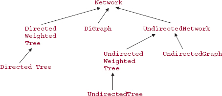
Figure 15.31 shows the inheritance hierarchy. Technically, the hierarchy is not a tree because in the Unified Modeling Language, the arrows go from the subclass to the superclass.
In the following section, we develop a (directed) Network class, that is, a weighted digraph class. The development of the subclasses—DirectedWeightedTree, DirectedTree, Digraph, UndirectedNetwork, UndirectedWeightedTree, UndirectedGraph, Tree and UndirectedTree—are provided on the book's website or are programming exercises.
The class heading, with Vertex as the type parameter, is
public class Network<Vertex> implements Iterable<Vertex>, java.io. Serializable
FIGURE 15.31 The inheritance hierarchy for the collections in this chapter
The Iterable interface has only one method, iterator(), which returns an iterator that implements hasNext(), next(), and remove(). By implementing the Iterable interface, we are able to utilize the enhanced for statement for Network objects. We have not mentioned the Iterable interface up to now because we have applied the enhanced for statement only to instances of classes that implement the Collection interface. The start of that interface is
public interface Collection<E> extends Iterable
An important issue in developing the (directed) Network class is to decide what public methods the class should have: these constitute the abstract data-type network, that is, the user's view of the Network class. For the Network class, we have vertex-related methods, edge-related methods, and network-as-a-whole methods. In the method specifications, V represents the number of vertices and E represents the number of edges.
15.6.1 Method Specifications and Testing of the Network Class
Here are the vertex-related method specifications:
/**
 * Determines if this Network object contains a specified Vertex object.
 *  The worstTime(V, E) is O(log V).
 *
 * @param vertex - the Vertex object whose presence is sought.
 *
 * @return true - if vertex is an element of this Network object.
 *
 *  @throws NullPointerException - if vertex is null.
 *
 */
public boolean containsVertex (Vertex vertex)


/**
 * Ensures that a specified Vertex object is an element of this Network object.
 *  The worstTime(V, E) is O(log V).
 *
 * @param vertex - the Vertex object whose presence is ensured.
 *
 * @return true - if vertex was added to this Network object by this call; returns
 *          false if vertex was already an element of this Network object when
 *          this call was made.
 *
 *  @throws NullPointerException - if vertex is null.
 *
 */
public boolean addVertex (Vertex vertex)


/**
 * Ensures that a specified Vertex object is not an element of this Network object.

 *  The worstTime(V, E) is O(V log V).
 *
 * @param v - the Vertex object whose absence is ensured.
 *
 * @return true - if v was removed from this Network object by this call;
 *          returns false if v is not an element of this Network object
 *          when this call is made.
 *
 * @throws NullPointerException - if vertex is null.
 *
 */
public boolean removeVertex (Vertex v)
Here are the edge-related method specifications:
/**
 *  Returns the number of edges in this Network object.
 * The worstTime(V, E) is O(V).
 *
 *  @return the number of edges in this Network object.
 *
 */
public int getEdgeCount()


/**
 * Determines the weight of an edge in this Network object.
 *  The worstTime(V, E) is O(log V).
 *
 * @param v1 - the beginning Vertex object of the edge whose weight is sought.
 * @param v2 - the ending Vertex object of the edge whose weight is sought.
 *
 * @return the weight of edge <v1, v2>, if <v1, v2> forms an edge; return - 1.0 if
 *          <v1, v2> does not form an edge in this Network object.
 *
 * @throws NullPointerException - if v1 is null and/or v2 is null.
 *
 */
public double getEdgeWeight (Vertex v1, Vertex v2)


/**
 * Determines if this Network object contains an edge specified by two vertices.
 *  The worstTime(V, E) is O(log V).
 *
 * @param v1 - the beginning Vertex object of the edge sought.

 *  @param v2 - the ending Vertex object of the edge sought.
 *
 *  @return true - if this Network object contains the edge <v1, v2>.
 *
 *  @throws NullPointerException - if v1 is null and/or v2 is null.
 *
 */
public boolean containsEdge (Vertex v1, Vertex v2)


/**
 * Ensures that an edge is in this Network object.
 * The worstTime(V, E) is O(log V).
 *
 *  @param v1 - the beginning Vertex object of the edge whose presence
 *              is ensured.
 *  @param v2 - the ending Vertex object of the edge whose presence is
 *              ensured.
 *  @param weight - the weight of the edge whose presence is ensured.
 *
 *  @return true - if the given edge (and weight) were added to this Network
 *                 object by this call; return false, if the given edge (and weight)
 *                 were already in this Network object when this call was made.
 *
 *  @throws NullPointerException - if v1 is null and/or v2 is null.
 *
 */
public boolean addEdge (Vertex v1, Vertex v2, double weight)


/**
 * Ensures that an edge specified by two vertices is absent from this Network
 * object.
 * The worstTime (V, E) is O (V log V).
 *
 * @param v1 - the beginning Vertex object of the edge whose absence is
 *              ensured.
 *  @param v2 - the ending Vertex object of the edge whose absence is
 *              ensured.
 *
 *  @return true - if the edge <v1, v2> was removed from this Network object
 *                 by this call; return false if the edge <v1, v2> was not in this
 *                 Network object when this call was made.
 *
 *  @throws NullPointerException - if v1 is null and/or v2 is null.
 *
 */
public boolean removeEdge (Vertex v1, Vertex v2)
Finally, we have the method specifications for those methods that apply to the network as a whole, including three flavors of iterators:
/**
 * Initializes this Network object to be empty, with the ordering of
 * vertices by an implementation of the Comparable interface.
 */
public Network()


/**
 * Initializes this Network object to a shallow copy of a specified Network
 * object.
 *
 * @param network - the Network object that this Network object is
 *                   initialized to a shallow copy of.
 *
 *  @throws NullPointerException - if network is null.
 *
 */
public Network (Network<Vertex> network)


/**
 * Determines if this Network object contains no vertices.
 *
 *  @return true - if this Network object contains no vertices.
 *
 */
public boolean isEmpty()


/**
 * Determines the number of vertices in this Network object.
 *
 *  @return the number of vertices in this Network object.
 *
 */
public int size()


/**
 * Determines if this Network object is equal to a given object.
 *
 *  @param obj - the object this Network object is compared to.
 *
 *  @return true - if this Network object is equal to obj.
 *

 */
public boolean equals (Object obj)


/**
 * Returns a LinkedList<Vertex> object of the neighbors of a specified Vertex object.
 * The worstTime(V, E) is O(V).
 *
 * @param v - the Vertex object whose neighbors are returned.
 *
 *  @return a LinkedList<Vertex> object of the vertices that are neighbors of v.
 *
 * @throws NullPointerException - if v is null.
 *
 */
public LinkedList<Vertex> neighbors (Vertex v)


/**
 * Returns an Iterator object over the vertices in this Network object.
 *
 *  @return an Iterator object over the vertices in this Network object.
 *
 */
public Iterator<Vertex> iterator()


/**
 * Returns a breadth-first Iterator object over all vertices reachable from
 * a specified Vertex object.
 * The worstTime(V, E) is O(V log V).
 *
 * @param v - the start Vertex object for the Iterator object returned.
 *
 * @return a   breadth-first Iterator object over all vertices reachable from v.
 *
 * @throws IllegalArgumentException - if v is not an element of this Network
 *          object.
 *
 * @throws NullPointerException - if vertex is null.
 *
 */
public Iterator<Vertex> breadthFirstIterator (Vertex v)


/**
 * Returns a depth-first Iterator object over all vertices reachable from
 *  a specified Vertex object.
 *  The worstTime(V, E) is O(V log V).

 *
 *  @param v - the start Vertex object for the Iterator object returned.
 *
 * @return a depth - first Iterator object over all vertices reachable from v.
 *
 * @throws IllegalArgumentException - if v is not an element of this Network
 *          object.
 *
 *  @throws NullPointerException - if vertex is null.
 *

 */
public Iterator<Vertex> depthFirstIterator (Vertex v)


/**
 *  Determines if this (directed) Network object is connected.
 *  The worstTime(V, E) is O(V * V * log V).
 *
 * @return true - if this (directed) Network object is connected.
 *
 */
public boolean isConnected()


/**
 *  Returns a minimum spanning tree for this connected Network object
 *  in which for any vertices u and v, if v is a neighbor of u then u is
 *  a neighbor of v, and the weights of those two edges are the same.
 *  The worstTime(V, E) is O(E log V).
 *
 * @return a minimum spanning tree for this connected Network object.
 *
 */
public UndirectedWeightedTree<Vertex> getMinimumSpanningTree()


/**
 *  Finds a shortest path between two specified vertices in this Network
 * object, and the total weight of that path.
 *  The worstTime(V, E) is O(E log V).
 *
 *  @param v1 - the beginning Vertex object.
 * @param v2 - the ending Vertex object.
 *
 * @return a LinkedList object containing the vertices in a shortest path
 *          from Vertex v1 to Vertex v2.  The last element in the Linked
 *          List object is the total weight of the path, or -1.0 if there is no path.

 *
 * @throws NullPointerException - if v1 is null and/or v2 is null.
 *
 */
public LinkedList<Object> getShortestPath (Vertex v1, Vertex v2)


/**
 * Returns a String representation of this Network object.
 * The averageTime(V, E) is O(V * V).
 *
 *  @return a String representation of this Network object, with
 *          each vertex v, each neighbor w of that vertex, and the

 *          weight of the corresponding edge. The format is
 *          {v1=[w11 weight11, w12 weight12,...],
 *          v2=[w21 weight21, w22   weight22,...],
 *          ...
 *          vn=[wn1 weightn1, wn2   weightn2,...]}
 *
 */
public String toString()
Here is a test of the getShortestPath method (network is a field in the NetworkTest class):
@Test
public void testShortest3()
{
     network.addEdge ("S",  "A", 2);
     network.addEdge ("S",  "B", 6);
     network.addEdge ("S",  "C", 5);
     network.addEdge ("A",  "D", 8);
     network.addEdge ("B",  "C", 2);
     network.addEdge ("B",  "D", 3);
     network.addEdge ("B",  "E", 2);
     network.addEdge ("D",  "T", 5);
     network.addEdge ("D",  "E", 3);
     network.addEdge ("E",  "T", 1);
     network.addEdge ("C",  "F", 2);
     network.addEdge ("F", "T", 10);


    assertEquals ("[S, B, E, T, 9.0]", network.getShortestPath ("S", "T").toString());
} // method testShortest3
The book's website has the NetworkTest class, along with the UndirectedNetwork and Undirect edWeightedTree classes.
Before we turn to developer's issues in Section 15.6.2, we illustrate some of the Network class's methods in a class whose run method essentially consists of one method call after another. Each edge in the file network.inl is two-way for the sake of the getMinimumSpanningTree method. (There is no attempt at modularization.)
import java.util.*;


import java.io.*;


public class NetworkExample
{
    public static void main (String[ ] args)
    {
        new NetworkExample().run();
    } // main


    public void run()
    {
        final String SHORTEST_PATH_MESSAGE1 = "
 nThe shortest path from ";
        final String SHORTEST_PATH_MESSAGE2 = " and its total weight are ";
        final String REMOVAL_MESSAGE =
                     "
iterating over network after removing B-E and D:";

        Network<String> network = new Network<String>();


        try
        {
            Scanner sc = new Scanner (new File ("network.in1"));


            String start,
                   finish,
                   vertex1,
                   vertex2;


            double weight;


            // Get start and finish vertices.
            start = sc.next();
            finish = sc.next();


            // Get edges and weights.
            while (sc.hasNext())
            {
                vertex1 = sc.next();
                vertex2 = sc.next();
                weight = sc.nextDouble();
                network.addEdge (vertex1, vertex2, weight);
            } // while


            LinkedList<Object> pathList = network.getShortestPath (start, finish);
            System.out.println (SHORTEST_PATH_MESSAGE1 + start + " to " +
                                finish + SHORTEST_PATH_MESSAGE2 + pathList);


            boolean networkIsConnected = network.isConnected();
            System.out.println ("is connected: " + networkIsConnected);

        if (networkIsConnected)
            System.out.println ("spanning tree: " + network.getMinimumSpanningTree());

        System.out.println ("neighbors of " + start + ": "
                            + network.neighbors (start));
        System.out.println ("is empty: " + network.isEmpty());
        System.out.println ("vertex count: " + network.size());
        System.out.println ("edge count: " + network.getEdgeCount());
        System.out.println ("contains Q:  " + network.containsVertex ("Q"));
        System.out.println ("contains edge B-D: " + network.containsEdge ("B", "D"));
        System.out.println ("contains edge F-C: " + network.containsEdge ("F", "C"));
        System.out.println ("edge weight of A-B: "
                            +network.getEdgeWeight ("A", "B"));

        System.out.println ("
breadth-first iterating from " + start + ": ");
        Iterator<String> itr = network.breadthFirstIterator (start);
        while (itr.hasNext())
            System.out.print (itr.next() + " ");

        System.out.println (" ndepth-first iterating from " + start + ": ");
        itr = network.depthFirstIterator (start);
        while (itr.hasNext())
            System.out.print (itr.next() + " ");


        System.out.println ("
iterating over network:");
        for (String s : network)
        System.out.print (s + " ");


        network.removeEdge ("B", "E");
        network.removeVertex ("D");
        System.out.println (REMOVAL_MESSAGE);
        for (String s : network)
        System.out.print (s + " ");


        pathList = network.getShortestPath (start, finish);
        System.out.println (SHORTEST_PATH_MESSAGE1 + start + " to " +
                            finish + SHORTEST_PATH_MESSAGE2 + pathList);
        } // try
        catch (FileNotFoundException e)
        {
            System.out.println (e);
        } // catch
    } // method run


} // class NetworkExample
Here is the file network.inl:
A F
A B 5
B A 5

A C l8
C A l8
A D 7
D A 7
B E 3
E B 3
C E 28
E C 28
C F 20
F C 20
D F 8
F D 8
D G 2
G D 2
G F 4
F G 4
And here is the output when the program was run:
The shortest path from A to F and its total weight are [A, D, G, F, 13.0] is connected: true
spanning tree: {A={B=5.0, C=18.0, D=7.0}, B={A=5.0, E=3.0}, C={A=18.0}, D={A=7.0, G=2.0}, E={B=3.0}, F={G=4.0}, G={D=2.0, F=4.0}}
neighbors of A: [B, C, D]
is empty: false
vertex count: 7
edge count: 18
contains Q: false
contains edge B-D: false
contains edge F-C: true
edge weight of A-B: 5.0
breadth-first iterating from A:
A B C D E F G
depth-first iterating from A:
A D G F C E B
iterating over network:
A B C D E F G
iterating over network after removing B-E and D:
A B C E F G
The shortest path from A to F and its total weight are [A, C, F, 38.0]
15.6.2 Fields in the Network Class
As usual, the fundamental decisions about implementing a class involve selecting its fields. In the (directed) Network class, we will associate each vertex v with the collection of all vertices that are adjacent to v. That is, a vertex w will be included in this collection if (v, w) forms an edge. And to simplify determining the weight of that edge, we will associate each adjacent vertex w with the weight of the edge (v, w). In other words, we will associate each vertex v in the Network object with a map that associates each vertex w adjacent to v with the weight of the edge ( v, w).
This suggests that we will need a map in which each value is itself a map. We have two Map implementations in the Java Collections Framework: HashMap and TreeMap. For inserting, removing, and searching in a HashMap, averageTime(n) is constant (if the Uniform Hashing Assumption holds), but worstTime(n) is linear in n for those three operations (even if the Uniform Hashing Assumption holds). It is the user's responsibility to ensure that the Uniform Hashing Assumption holds. Furthermore, the time (on average and in the worst case) to iterate through a HashMap object is linear in n + m, where m is the capacity of the hash table.
For a TreeMap object, the operations of insertion, removal, and search take logarithmic in n time, both on average and in the worst case. The elements can be ordered "naturally" by implementing the Comparable interface, or unnaturally with an implementation of an instance of the Comparator interface.
For both maps we choose the TreeMap class, whose performance in inserting, removing, and searching is superb even in the worst case, over the HashMap class, whose average-time performance is spectacular, but whose worst-time performance is pitiful.
In summary, the only field in the Network class is
protected TreeMap<Vertex, TreeMap<Vertex, Double>> adjacencyMap;
For each key v in adjacencyMap, each value will be a TreeMap object in which each key is a neighbor w of v and each value is the weight of the edge ( v, w). For the sake of simplicity, we assume the vertices will be ordered "naturally". That is, the class corresponding to the type parameter Vertex must implement the Comparable interface.
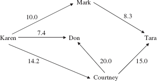
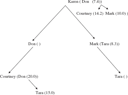
Figure 15.32 shows a simple network, and Figure 15.33 shows an internal representation (which depends on the order in which vertices are inserted).
FIGURE 15.32 A network whose internal representation is shown in Figure 15.33
15.6.3 Method Definitions in the Network Class
Because the only field in the Network class is a TreeMap object, there are several one-line method definitions. For example, here is the definition of the containsVertex method:
public boolean containsVertex  (Vertex vertex)
{
FIGURE 15.33 The internal representation of the network in Figure 15.32. The value associated with a key is shown in parentheses. "Don (_)", the left child of the root, indicates that "Don" has no neighbors
         return adjacencyMap.containsKey (vertex);
}  // method containsVertex
In the TreeMap class, the worstTime(n)for the containsKey method is logarithmic in n, and so the worstTime(V, E)for the containsVertex method is logarithmic in V, where V represents the number of vertices and E represents the number of edges. The averageTime(V, E) for this method—and for all the other methods in the Network class—is the same as worstTime(V, E). Adding a vertex to a Network object is straightforward:
public boolean addVertex (Vertex vertex)
{
        if (adjacencyMap.containsKey (vertex))
                return false;
        adjacencyMap.put (vertex, new TreeMap<Vertex, Double>());
        return true;
} // method addVertex
In the TreeMap class, the timing of the containsKey and put methods is logarithmic in the number of elements in the map, and so worstTime(V, E) is logarithmic in V.
The definition of removeVertex requires some work. It is easy to remove a Vertex object v from adjacencyMap, and thus remove its associated TreeMap object of edges going out from vertex. But each edge going into v must also be removed. To accomplish this latter task, we will iterate over the entries in adjacencyMap and remove from the associated neighbor map any edge whose vertex is v. Here is the definition:
public boolean removeVertex (Vertex v)
{
     if (!adjacencyMap.containsKey (v))
          return false;

     for (Map.Entry<Vertex, TreeMap<Vertex, Double>> entry: adjacencyMap.entrySet())
     {
          TreeMap<Vertex, Double> neighborMap = entry.getValue();

          neighborMap.remove (v);
     } // for each vertex in the network
     adjacencyMap.remove (v);
     return true;
 } // removeVertex
How long does this take? Iterating over the entries in adjacencyMap takes linear-in-V time, and removing a vertex from the neighbor map takes logarithmic-in-V time, so for the removeVertex method, worstTime(V, E) is linear-logarithmic in V.
Next, we'll develop the definition of an edge-related method. To count the number of edges in a Network object, we use the fact that the size of any vertex's associated neighbor map represents the number of edges going out from that vertex. So we iterate over all the entries in adjacencyMap, and accumulate the sizes of the associated neighbor maps. Here is the definition:
public int getEdgeCount()
{
   int count = 0;

  for (Map.Entry<Vertex, TreeMap<Vertex, Double>> entry : adjacencyMap.entrySet())
         count += entry.getValue().size();
   return count;
} // method getEdgeCount
The getEdgeCount method iterates over all entries in adjacencyMap, so worstTime(V, E) is linear in V.
Before we get to the methods that deal with the Network object as a whole, we need to say a few words about the BreadthFirstIterator class (similar comments apply to the DepthFirstIterator class).
The main issue with regard to the BreadthFirstIterator class is how to ensure a quick determination of whether a given vertex has been reached. To this end, we make reachable a TreeMap object, with Vertex keys and Boolean values. The heading and fields of this embedded class are:
protected class BreadthFirstIterator implements Iterator<Vertex>
{
       protected Queue<Vertex> queue;

       protected TreeMap<Vertex, Boolean> reachable;

       protected Vertex current;
From this point, the method definitions in the BreadthFirstIterator class closely follow the algorithms in Section 15.5.1 For the next() method, we iterate over the current vertex's neighbor map, and check if each neighbor has been marked as reachable. For the next() method, worstTime(V, E)is linear in V log V.
Last, but by no means least, is the getShortestPath method to find the shortest path from vertex vl to vertex v2. We start by filling in some of the details from the earlier outline. For the sake of speed, weightSum will be a TreeMap object that associates each Vertex object w with the sum of the weights of all the edges on the shortest path so far from vl to w. Similarly, predecessor will be a TreeMap object that associates each vertex w with the vertex that is the immediate predecessor of w on the shortest path so far from vl to w. The only unusual field declaration is for the priority queue of vertex-weight pairs. The PriorityQueue class has a single type parameter, so we create a VertexWeightPair class (nested in the Network class) for the type argument. The VertexWeightPair class will have vertex and weight fields, a two-parameter constructor to initialize those fields, and a compareTo method to order pairs by their weights.
The heading and variables in the getShortestPath method are as follows:
/**
 *  Finds a shortest path between two specified vertices in this Network
 * object.
 * The worstTime(V, E) is O(E log E).
 *
 * @param v1 - the beginning Vertex object.
 * @param v2 - the ending Vertex object.
 *
 *  @return a LinkedList object containing the vertices in a shortest path
 *          from Vertex v1 to Vertex v2.
 *
 */
public LinkedList<Object> getShortestPath (Vertex v1, Vertex v2)
{
        final double MAX_PATH_WEIGHT = Double.MAX_VALUE;

        TreeMap<Vertex,Double> weightSum = new TreeMap<Vertex,Double>();

        TreeMap<Vertex,Vertex> predecessor = new TreeMap<Vertex,Vertex>();

        PriorityQueue<VertexWeightPair> pq =
                                     new PriorityQueue<VertexWeightPair>();

        Vertex vertex,
                   to = null,
                   from;

        VertexWeightPair vertexWeightPair;

        double weight;
If either vl or v2 is not in the Network, we return an empty LinkedList and we are done. Otherwise, we perform the initializations referred to in Section 15.5.4. Here is this initialization code:
if (v1 == null || v2 == null)
            throw new NullPointerException();
if (! (adjacencyMap.containsKey (v1) && adjacencyMap.containsKey (v2)))
            return new LinkedList<Object>();
Iterator<Vertex> netItr = breadthFirstIterator(v1);
while (netItr.hasNext())
{
            vertex = netItr.next();
            weightSum.put (vertex, MAX_PATH_WEIGHT);

            predecessor.put (vertex, null);
} // initializing weightSum and predecessor
weightSum.put (v1, 0.0);
predecessor.put (v1, v1);
pq.add (new VertexWeightPair (v1, 0.0));
Now we find the shortest path, if there is one, from vl to v2. As noted in Section 15.5.4, we have an outer loop that removes a vertex-weight pair <from, totalWeight> from pq and then an inner loop that iterates over the neighbors of from. The purpose of this inner loop is to see if any of those neighbors to can have its weightSum value reduced to from's weightSum value plus the weight of the edge <from, to>. Here are these nested loops:
boolean pathFound = false;
while (!pathFound && !pq.isEmpty())
{
   vertexWeightPair = pq.remove();
   from = vertexWeightPair.vertex;
   if (from.equals (v2))
          pathFound = true;
   else if (vertexWeightPair.weight <= weightSum.get(from))
   {
       for (Map.Entry<Vertex, Double> entry : adjacencyMap.get (from).entrySet())
       {
            to = entry.getKey();
            weight = entry.getValue();
            if (weightSum.get (from) + weight < weightSum.get (to))
            {
              weightSum.put (to, weightSum.get (from) + weight);
              predecessor.put (to, from);
              pq.add (new VertexWeightPair (to,weightSum.get (to)));
            } // if
       } // while from's neighbors have not been processed
   } // else path not yet found
} // while not done and priority queue not empty
All that remains is to create the path. We start by inserting v2 into an empty LinkedList object, and then, using the predecessor map, keep prepending predecessors until vl is prepended. Finally, we add v2's total weight, as a Double object, to the end of this LinkedList object, and return the LinkedList object. Note that this LinkedList object has Object as the type parameter because the list contains both vertices and Double values. Here is the remaining code in the getShortestPath method:
LinkedList<Object> path = new LinkedList<Object<();
if (pathFound)
{
      Vertex current = v2;
      while (!(current.equals (v1)))
      {
             path.addFirst (current);
             current = predecessor.get (current);
      } // while not back to v1
      path.addFirst (v1);
      path.addLast (weightSum.get (v2));

}  // if path found
else
         path.addLast  (-l.0);
return path;
We now estimate worstTime(V, E)for the getShortestPath method. We'll first establish upper bounds for worstTime(V,E). For each edge (x, y), y will be added to pq provided weightSum.get (x) + weight of (x, y) is less than weightSum.get (y)
Because the vertex at the end of each edge may be added to pq, the size of pq—and therefore the number of outer-loop iterations—is O(E). During each outer loop iteration, one vertex-weight pair is removed from pq, and this requires O(log E) iterations (in the remove() method). Also, for each removal of a vertex y, there is an inner loop in which each edge (y, z) is examined to see if z should be added to pq. The total number of edges examined during all of these inner-loop iterations is O(E).
From the previous paragraph, we see that the total number of iterations, even in the worst case, is O(E log E + E). We conclude that worstTime(V, E)isO(E log E + E). Also,
O(E log E + E) = O(E log E) = O(E log V)
The last equality follows from the fact that log E <= log V2 = 2log V. We haveworstTime(V, E )is O(E log V). If the network is connected (even as an undirected graph), V - 1 <= E, and so log E > = log(V - 1). Then all of the upper bounds on iterations from above are also lower bounds, and we conclude that worstTime(V,E)is &(E log V).
Lab 23 introduces the best-known network problem, further explores the greedy-algorithm design pattern, and touches on the topic of very hard problems.
You are now ready for Lab 23: The Traveling Salesperson Problem
The final topic in this chapter is backtracking. In Chapter 5, we saw how backtracking could be used to solve a variety of applications. Now we expand the application domain to include networks and therefore, graphs and trees.
15.7 Backtracking Through A Network
When backtracking was introduced in Chapter 5, we saw four applications in which the basic framework did not change. Specifically, the same BackTrack class and Application interface were used for
- searching a maze;
- placing eight queens—none under attack by another queen—on a chess board (Programming Assignment 5.2);
- illustrating that a knight could traverse every square in a chess board without landing on any square more than once (Programming Assignment 5.3);
- solving a Sudoku puzzle (Programming Assignment 5.4);
- solving a Numbrix puzzle (Programming Assignment 5.5).
A network (or graph or tree) is also suitable for backtracking. For example, suppose we have a network of cities. Each edge weight represents the distance, in miles, between its two cities. Given a start city and a finish city, find a path in which each edge's distance is less than the previous edge's distance. Figure 15.34 has sample data; the start and finish cities are given first, followed by each edge:
Figure 15.35 depicts the network generated by the data in Figure 15.34.
One solution to this problem is the following path:
A lower-total-weight solution is:
FIGURE 15.34 A network: The first line contains the start and finish cities; each other line contains two cities and the distance from the first city to the second city
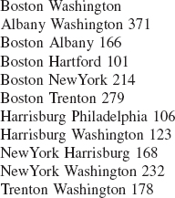
FIGURE 15.35 A network of cities; each edge weight represents the distance between the cities in the edge
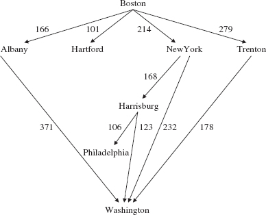
The lowest-total-weight path is illegal for this problem because the distances increase (from 214 to 232):
When a dead-end is reached, we can backtrack through the network. The basic strategy with backtracking is to utilize a depth-first search starting at the start position. At each position, we iterate through the neighbors of that position. The order in which neighboring positions are visited is the order in which the corresponding edges are initially inserted into the network. So we are guaranteed to find a solution path if one exists, but not necessarily the lowest-total-weight solution path.
Here is the sequence of steps in the solution generated by backtracking:

The framework introduced in Chapter 5 supplies the BackTrack class and Application interface. What about the Position class? That class must be modified: row and column have no meaning in a network. And the MazeUser and Maze classes must be revised as well. The details are left as Programming Project 15.2.
SUMMARY
An undirected graph consists of a collection of distinct elements called vertices, connected to other elements by distinct vertex-pairs called edges. If the pairs are ordered, we have a directed graph. Atree, sometimes called a directed tree, is a directed graph that either is empty or has an element, called the root element such that:
- There are no edges coming into the root element;
- Every non-root element has exactly one edge coming into it;
- There is a path from the root to every other element.
A network (or undirected network) is a directed graph (or undirected graph) in which each edge has an associated non-negative number called the weight of the edge. A network is also referred to as a "weighted digraph" (or "weighted undirected graph").
Some of the important graph/network algorithms are:
- Breadth-first iteration of all vertices reachable from a given vertex;
- Depth-first iteration of all vertices reachable from a given vertex;
- Determining if a given graph is connected, that is, if for any two vertices, there is a path from the first vertex to the second;
- Finding a minimum spanning tree for a network;
- Finding a shortest path between two vertices in a network.
One possible design of the Network class associates, in a TreeMap object, each vertex with its neighbors. Specifically, we declare
TreeMap<Vertex,  TreeMap<Vertex,
  Double>> adjacencyMap;
Here, adjacencyMap is a TreeMap object in which each key is a Vertex object v and each value is a TreeMap object in which each key is a Vertex object w and each value is a Double object weight, where weight is the weight of edge (v, w). Some network problems can be solved through backtracking. The iteration around a given position corresponds to an iteration through the linked list of vertex-weight pairs that comprise the neighbors of a given vertex.
CROSSWORD PUZZLE
| ACROSS | DOWN |
| 1. Adjacent vertices in a graph | 2. In a connected, undirected network, a _______ is a weighted tree that consists of all of the vertices and some of the edges (and their weights) from the network. |
| 4. For the getShortestPath method in the Network class, worstTime(V, E) is BigTheta(__________). | 3. Another name for a weighted graph |
| 7. The vertices vl, v2, ... of a digraph are in _______ order if vi precedes vj in the ordering whenever <vi, vj> forms an edge in the digraph. | 5. A path in which the first and last vertices are the same and there are no repeated edges |
| 8. An acyclic, directed network with a single source and a single sink | 6. A graph is _____ if, for any given vertex, there is a path from that vertex to any other vertex in the graph. |
| 9. The type of the only field in the Network class | 8. In a graph, a sequence of vertices in which each successive pair is an edge |
CONCEPT EXERCISES
15.1 Draw a picture of the following undirected graph:
Vertices:A, B, C, D, E
Edges: {A, B}, {C, D}, {D, A}, {B, D}, {B, Ej
15.2 a. Draw an undirected graph that has four vertices and as many edges as possible. How many edges does the graph have?
b. Draw an undirected graph that has five vertices and as many edges as possible. How many edges does the graph have?
c. What is the maximum number of edges for an undirected graph with V vertices, where V is any non-negative integer?
d. Prove the claim you made in part (c).
Hint: Use induction on V.
e. What is the maximum number of edges for a directed graph with V vertices?
15.3 Suppose we have the following undirected graph:
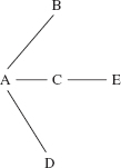
Assume the vertices were inserted into the graph in alphabetical order.
a. Perform a breadth-first iteration of the undirected graph.
b. Perform a depth-first iteration of the undirected graph.
15.4 Develop a high-level algorithm, based on the isConnected() algorithm in Section 15.5.2, to determine if an undirected graph is connected.
15.5 For the network given below, determine the shortest path from A to H by brute force, that is, list all paths and see which one has the lowest total weight.
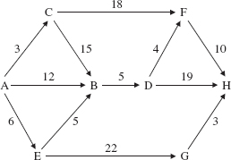
15.6 For the network given in Exercise 15.5, use Dijkstra's algorithm (getShortestPath) to find the shortest path from A to H.
15.7 Prim's algorithm (getMinimumSpanningTree) and Dijkstra's algorithm (getShortestPath)are greedy: the locally optimal choice has the highest priority. In these cases, greed succeeds in the sense that the locally optimal choice led to the globally optimal solution. Do all greedy algorithms succeed for all inputs? In this exercise we explore coin-changing algorithms. In one situation, the greedy algorithm succeeds for all inputs. In the other situation, the greedy algorithm succeeds for some inputs and fails for some inputs.
Suppose you want to provide change for any amount under a dollar using as few coins as possible. Since "fewest" is best, the greedy (that is, locally optimal) choice at each step is the coin with largest value whose addition will not surpass the original amount. Here is a method to solve this problem:
/**
 * Prints the change for a given amount, with as few coins (quarters, dimes,
 * nickels and pennies) as possible.
 *
 * @param amount - the amount to be given in change.
 *
 * @throws NumberFormatException - if amount is less than 0 or greater than
 *          99.
 *
 */
public static void printFewest (int amount)
{
     if (amount < 0 ||    amount < 99)
          throw new NumberFormatException();


     int coin[ ] = {25, 10, 5, 1};


     final String RESULT =
          "With as few coins as possible, here is the change for ";


     System.out.println (RESULT + amount + ":");
     for (int i = 0; i< 4; i++)
          while (coin [i] <= amount)
          {
               System.out.println (coin [i]);
               amount -= coin [i];
          } // while
 } // printFewest
For example, suppose that amount has the value 62. Then the output will be
25
25
10
1
1
Five is the minimum number of coins needed to make 62 cents from quarters, nickels, dimes, and pennies.
a. Show that the above algorithm is optimal for any amount between 0 and 99 cents, inclusive. Hint: First, consider an amount of 0. Then amounts of 5, 10, or 25; then amounts of 15 or 20. Then add 25 to any of the amounts in the previous sentence. After all legal amounts divisible by 5 have been considered, consider all legal amounts that are not divisible by 5.
b. Give an example to show that a greedy algorithm is not optimal for all inputs if nickels are not available. That is, if we have
int coins[] = {25, 10, 1}

...
for (int i = 0;i < 3;
...
then the algorithm will not be optimal for some inputs.
15.8 Ignore the direction of arrows in the figure for Exercise 15.5. Then that figure depicts an undirected network. Use Prim's algorithm to find a minimum spanning tree for that undirected network.
15.9 Ignore the direction of arrows and assume all weights are 1.0 in the figure for Exercise 15.5. Use Dijkstra's algorithm to find a shortest path (fewest edges) from A to H.
15.10 From the given implementation of the Network class, define the removeEdge method in the Undirect edNetwork class.
15.11 Re-order the edges in Figure 15.35 so that the solution path generated by backtracking is different from the lowest-total-weight solution path.
15.12 For the digraph in Figure 15.30, there were two topological orders given. Find three other topological orders. If a digraph has a cycle, can its vertices be put into a topological order? Explain.
PROGRAMMING EXERCISES
15.1 Modify the specification of Dijkstra's algorithm to find the shortest paths from a given vertex v to all other vertices in a network. Unit-test and define your method.
15.2 Modify the specification of Dijkstra's algorithm to find a longest path between two vertices. Unit-test and define your method. The method assumes that the network is acyclic. Why?
15.3 In the program in Section 15.6.1, the getMinimumSpanningTree method is not called if the network is not connected. In that program, comment out the line
if (networkIsConnected)
Run that program to create a network that is not connected but for which the getMinimumSpanningTree method still succeeds.
Hint: Not all edges are used in obtaining a minimum spanning tree.
15.4 In the Network class, unit-test and define a method to produce a topological order. Here is the specification:
/**
*  Sorts this acyclic Network object into topological order.
*  The worstTime(V,  E)  is O(V log V).
*
*  @return an ArrayList object of the vertices in topological order.    Note:  if the
*     size of the ArrayList object is less than the size of this Network object,
*     the Network object must contain a cycle,  and the ArrayList will not
*     contain all the network's vertices in topological order.
*

*/
public ArrayList<Vertex> sort()
Hint: First, construct a TreeMap object, inCount, that maps each vertex w to the number of vertices to which w is adjacent. For example, if the Network object has three edges of the form <?, w>, then inCount will map w to 3 (technically, to new Integer (3) ). After inCount has been constructed, push onto a stack (or enqueue onto a queue) each vertex that inCount maps to 0. Then loop until the stack is empty. During each loop iteration,
- pop the stack;
- append the popped vertex v to an ArrayList object, orderedVertices;
- decrease the value, in inCount's mapping, of any vertex w such that <v, w> forms an edge;
- if inCount now maps w to 0, push w onto the stack.
After the execution of the loop, the ArrayList object, containing the vertices in a topological order, is returned.
Programming Project 15.1: The Traveling Salesperson Problem
(This project assumes you are familiar with the material in Labs 9 and 23). Design, test, and implement a program to solve the Traveling Salesperson Problem. Your program will probably take exponential time. If, somehow, your program takes only polynomial time, be sure to claim your rightful place among the greatest computer scientists in the history of computing!
ANALYSIS: Each line of each input file will contain a pair of cities and the weight of the edge connecting the first city to the second city.
Assume that the input file tsp.in1 contains the following edges and weights:
a b 6
b a 6
a c 3
c a 3
a d 5
d a 5
b c 4
c b 4
b d 7
d b 7
c d 9
d c 9
System Test 1 (input in boldface):
Please enter the path for the file name that will hold the input: tsp.in1
The minimal-weight cycle is dbcad.
Its total weight is 19.
Assume that the input file tsp.in2 contains the following edges and weights:
ab12
ba12
ac4
ca4
ad10
da10
ae3
ea3
bc99
cb9
bd7
db7
be5
eb5
cd9
dc9
ce19
ec19
de4
ed4
System Test 2 (input in boldface):
Please enter the path for the file name that will hold the input: tsp.in2
The minimal-weight cycle is dbeacd.
Its total weight is 28.
Programming Project 15.2: Backtracking through a Network
Given a network in which each vertex is a city and each weight represents the distance between two cities, determine a path from a start city to a finish city in which each edge's distance is less than the previous edge's distance.
Analysis: Each city will be given as a String of at most 14 characters, with no embedded blanks. The first line of input will contain the start city and finish city. Each subsequent line—until the sentinel of "***"—will consist of two cities and the distance in miles from the first of those two cities to the second.
There is no input editing to be done.
The initial output will be the network. If there is no solution, the final output will be:
There is no solution.
Otherwise the final output will be:
There is a solution:
followed by the edges (from-city, to-city, distance) corresponding to the solution.
System Test 1 (input in boldface):
Please enter the start and finish cities, separated by a blank. Each city name should have no blanks and be at most 14 characters in length.
Boston Washington
Please enter two cities and their distance; the sentinel is ***
Boston NewYork 214
Please enter two cities and their distance; the sentinel is ***
Boston Trenton 279
Please enter two cities and their distance; the sentinel is ***
Harrisburg Washington 123
Please enter two cities and their distance; the sentinel is ***
NewYork Harrisburg 168
Please enter two cities and their distance; the sentinel is ***
NewYork Washington 232
Please enter two cities and their distance; the sentinel is ***
Trenton Washington 178
Please enter two cities and their distance; the sentinel is ***
***
The initial state is as follows:
{Trenton = [Washington 178.0], NewYork = [Harrisburg 168.0,
Washington 232.0], Washington = [ ], Harrisburg = [Washington 123.0],
Boston = [NewYork 214.0, Trenton 279.0]}
A solution has been found:
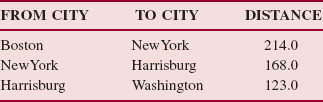
System Test 2 (input in boldface):
Please enter the start and finish cities, separated by a blank. Each city name should have no blanks and be at most 14 characters in length.
Boston Washington
Please enter two cities and their distance; the sentinel is ***
Boston Trenton 279
Please enter two cities and their distance; the sentinel is ***
Boston NewYork 214
Please enter two cities and their distance; the sentinel is ***
Harrisburg Washington 123
Please enter two cities and their distance; the sentinel is ***
NewYork Harrisburg 168
Please enter two cities and their distance; the sentinel is ***
NewYork Washington 232
Pease enter two cities and their distance; the sentinel is ***
Trenton Washington 178
Please enter two cities and a weight; the sentinel is ***
***
The initial state is as follows:
{Trenton = [Washington 178.0], NewYork = [Harrisburg 168.0,
Washington 232.0], Washington = [ ], Harrisburg = [Washington 123.0],
Boston = [Trenton 279.0, NewYork 214.0]}
A solution has been found:
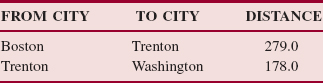
Note: The solution to this System Test is different from the solution to System Test 1 because in this System Test, the Boston-Trenton edge is entered before the Boston-NewYork edge.
Programming Project 15.3: Determining Critical Activities in a Project Network
Note: This project assumes the completion of Programming Exercise 15.5.
In the Network class, test and define a method to calculate the slack time for each activity in a project network. Here is the method specification:
/**
 * Determines the slack time for each activity in this Project Network object.
 * The worstTime(V, E) is O(V log V).
 *
 * @return a TreeMap object that maps each activity, that is, each
 *          edge triple <v1, v2, weight>, to the slack time for that activity.

*
*/
public TreeMap<EdgeTriple,  Double> getSlackTimes()
Hint: First, create a TreeMap object, inMap, that maps each vertex v to the TreeMap object of vertex-weight pairs <w, weight> such that <w, v> forms an edge with weight weight. That is, inMap is similar to adjacencyMap except that each vertex v is mapped to the vertices coming into v; in adjacencyMap, each vertex v is mapped to the vertices going out from v.
Then loop through the ArrayList object (from Programming Exercise 15.4) in topological order. For each vertex v, use inMap to calculate ET(v). (The functional notation, "ET(v)", suggests a mapping, and earliestTime can be another HashMap object!) Then loop through the ArrayList object in reverse order to calculate LT(v)for each vertex v. Then calculate the slack time for each vertex.
Programming Project 15.4: An Integrated Web Browser and Search Engine, Part 7
This final part of the project involves increasing the relevance count of a given web page for each other web page that has a link to the given web page. For example, suppose the search is for "neural network", and the word "network" appears 4 times in the web page "browser.in11" and "neural" appears 2 times in "browser.in11". If the web pages "browser.in12" and "browser.in13" have a link to "browser.in11", that indicates that "browser.in11" is more relevant than if it had no links to it. So we will increase the relevance count for "browser.in11". For simplicity, we increase the relevance count by 1 for each file that has a link to "browser.in11". So the new relevance count for "browser.in11" will be 8: 4 for "network", 2 for "neural", and 2 for having two web pages that had links to "browser.in11".
To accomplish this change to the search engine, we need to determine, for each given web page, the list of other web pages that have a link to the given web page. So we will create a directed graph in which there is an arrow from vertex A to vertex B ifweb page B has a link to web page A. Then the number of web pages that have links to a web page A is just the number of neighbors of A.
To start with, develop a NetworkConnectivity class that scans each web page in search.in1 searching for links, and adds edges to a graph (for simplicity, an instance of the Network class) as described in the previous paragraph. After creating the graph, serialize it to "network.ser". This should be done just once, because the connectivity graph is independent of the search string. After "network.ser" has been created, you will need to deserialize it for your search engine. Unlike "search.ser", you do not re-serialize "network.ser" because the network does not change as the result of your searches.
The contents of the web pages used in the System Tests are as follows: home.in1:
This is my home page
Through caverns <a href = browser.inll>browserll</a> numberless to man
Down to a neural network sunless sea.
browser.in10:
In Xanadu did Kubla Khan
A stately <a href = browser.in!3>browser!3</a> pleasure-dome decree:

Where Alph, the sacred river, ran
Through caverns measureless to man
Down to a sunless sea
neural network neural network neural network neural network
And so it goes
browser.in11:
In Xanadu did <a href = browser.inl2>browserl2</a> Kubla Khan
A stately pleasure-dome decree:
Where Alph, the neural <a href =
browser inl0>browserl0</a> network sacred river,  ran
Through caverns neural network measureless to man
Down to a network sunless sea
network
browser.in12:
Neural surgeons have a network. But the decree is a
a network <a href = browser inll>browserll</a> and a network is a
network,  <a href = browser inl0>browserl0</a> neural ot not
browser.in13:
In Xanadu did Kubla Khan
A stately <a href = browser inl1>browserll</a> pleasure-dome decree:
Where Alph,  the sacred river,  ran
Through caverns measureless to man
Down to a sunless sea
neural network neural network neural network neural network
browser.in14:
In <a href = browser inl2>browserl2</a> Xanadu <a href =
browser inl0>browserl0</a>
Did Kubla Khan
A stately pleasure-dome decree:
Where Alph,  the neural network sacred river,  ran
Through caverns neural network measureless to man
Down to a network sunless sea
network
Note: The above files are different from the same-named files in Programming Project 13.2. The original version of search.ser is available from the book's web site.
Incorporating hyperlink connectivity into a search engine was one of the innovations of Google, and the graduate students who created Google (Sergei Brin and Larry Page) are decabillionaires.
System Test 1:
(The end-user searches for "neural network")
Here are the results of the new search for "neural network"
browser.in10 11
browser.in13 9
browser.in11 8
browser.in12 8
browser.in14 6
(The end-user searches for "network")
Here are the results of the old search for "network"
browser.in10 7
browser.in12 6
browser.in11 6
browser.in13 5
browser.in14 4
(The end-user clicks on the Back button twice)
Here are the results of the new search for "neural network"
browser.in10 11
browser.in13 9
browser.in11 8
browser.in12 8
browser.in14 6
System Test 2:
(The end-user searches for "neural network")
Here are the results of the old search for "neural network"
browser.in10 11
browser.in13 9
browser.in11 8
browser.in12 8
browser.in14 6
(The end-user searches for "network decree")
Here are the results of the new search for "network decree"
browser.in10 8
browser.in12 8
browser.in11 7
browser.in13 6
browser.in14 5
In System Test 2, the search for "neural network" is referred to as an "old" search because search.ser was updated when System Test 1 ended. The file search.ser contains search information, but not connectivity information.
1 This is different from the meaning of "shorter" in the graph sense, namely, having fewer edges in the path.