
CHAPTER 11
Sorting
One of the most common computer operations is sorting, that is, putting a collection of elements in order. From simple, one-time sorts for small collections to highly efficient sorts for frequently used mailing lists and dictionaries, the ability to choose among various sort methods is an important skill in every programmer's repertoire.
CHAPTER OBJECTIVES
- Compare the Comparable interface to the Comparator interface, and know when to use each one.
- Be able to decide which sort algorithm is appropriate for a given application.
- Understand the limitations of each sort algorithm.
- Explain the criteria for a divide-and-conquer algorithm.
11.1 Introduction
Our focus will be on comparison-based sorts; that is, the sorting entails comparing elements to other elements. Comparisons are not necessary if we know, in advance, the final position of each element. For example, if we start with an unsorted list of 100 distinct integers in the range 0 … 99, we know without any comparisons that the integer 0 must end up in position 0, and so on. The best- known sort algorithm that is not comparison-based is Radix Sort: see Section 11.5.
All of the sort algorithms presented in this chapter are generic algorithms, that is, static methods: they have no calling object and operate on the parameter that specifies the collection to be sorted. Two of the sort methods, Merge Sort and Quick Sort, are included in the Java Collections Framework, and can be found in the Collections or Arrays classes in the package java.util.
The parameter list may include an array of primitive values (ints or doubles, for example), an array of objects, or a List object—that is, an instance of a class that implements the List interface. In illustrating a sort algorithm, we gloss over the distinction between an array of ints, an array of Integer objects and a List object whose elements are of type Integer. In Section 11.3, we'll see how to sort objects by a different ordering than that provided by the compareTo method in the Comparable interface.
In estimating the efficiency of a sorting method, our primary concerns will be averageTime(n) and worstTime(n). In some applications, such as national defense and life-support systems, the worst-case performance of a sort method can be critical. For example, we will see a sort algorithm that is quite fast, both on average and in the worst case. And we will also look at a sort algorithm that is extremely fast, on average, but whose worst-case performance is achingly slow.
The space requirements will also be noted, because some sort algorithms make a copy of the collection that is to be sorted, while other sort algorithms have only negligible space requirements.
Another criterion we'll use for measuring a sort method is stability. A stable sort method preserves the relative order of equal elements. For example, suppose we have an array of students in which each student consists of a last name and the total quality points for that student, and we want to sort by total quality points. If the sort method is stable and before sorting, ("Balan", 28) appears at an earlier index than ("Wang", 28), then after sorting ("Balan" 28) will still appear at an earlier index than ("Wang" 28). Stability can simplify project development. For example, assume that the above array is already in order by name, and the application calls for sorting by quality points; for students with the same quality points the ordering should be alphabetical. A stable sort will accomplish this without any additional work to make sure students with the same quality points are ordered alphabetically.
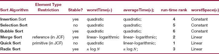
Table 11.1 at the end of the chapter provides a summary of the sorting methods we will investigate.
Each sort method will be illustrated on the following collection of 20 int values:
59 46 32 80 46 55 50 43 44 81 12 95 17 80 75 33 40 61 16 87
Here is the method specification and one of the test cases for the ?Sort method, where ?Sort can represent any of the sort methods from Section 11.2:
/**
  *  Sorts a specified array of int values into ascending order.
  *  The worstTime(n) is O(n * n).
  *
  *  @param x - the array to be sorted.
  *
  *  @throws NullPointerException - if x is null.
  *
  */
public static void ?Sort (int[] x)

public void testSample()
{
     int [ ] expected = {12, 16, 17, 32, 33, 40, 43, 44, 46,
                  50, 55, 59, 61, 75, 80, 80, 81, 87,  95};
     int [ ] actual = {59, 46, 32, 80, 46, 55, 50, 43, 44, 81,
                  12, 95, 17, 80, 75, 33, 40, 61, 16,  87};
     Sorts.?Sort (actual);
     assertArrayEquals (expected, actual);
} // method testSample
The remaining test cases can be found on the book's website.
11.2 Simple Sorts
We'll start with a few sort algorithms that are fairly easy to develop, but provide slow execution time when n is large. In each case, we will sort an array of int values into ascending order, and duplicates will be allowed. These algorithms could easily be modified to sort an array of doubles, for example, into ascending order or into descending order. We could also sort objects in some class that implements the Comparable interface. The ordering, provided by the compareTo method, would be "natural": for example, String objects would be ordered lexicographically. In Section 11.3, we'll see how to achieve a different ordering of objects than the one provided by the compareTo method.
11.2.1 Insertion Sort
Insertion Sort repeatedly sifts out-of-place elements down into their proper indexes in an array. Given an array x of int values, x [1] is inserted where it belongs relative to x [0], so x [0], and x [1] will be swapped if x [0] > x [1]. At this point, we have x [0] <= x [1]. Then x [2] will be inserted where it belongs relative to x [0] and x [1]; there will be 0, 1 or 2 swaps. At that point, we have x [0] <= x [1] <= x [2]. Then x [3] will be inserted where it belongs relative to x [0] ... x [2]. And so on.
Example Suppose the array x initially has the following values:
59 46 32 80 46 55 50 43 44 81 12 95 17 80 75 33 40 61 16 87
We first place x [1], 46, where it belongs relative to x [0], 59. One swap is needed, and this gives us:
46 59 32 80 46 55 50 43 44 81 12 95 17 80 75 33 40 61 16 87
The underlined values are in their correct order. We then place x [2], 32, where it belongs relative to the sorted subarray x [0] ... x [1], and two swaps are required. We now have
32 46 59 80 46 55 50 43 44 81 12 95 17 80 75 33 40 61 16 87
Next, we place x [3], 80, where it belongs relative to the sorted subarray x [0] ... x [2]; this step does not require any swaps, and the array is now
32 46 59 80 46 55 50 43 44 81 12 95 17 80 75 33 40 61 16 87
We then place x [4], 46, where it belongs relative to the sorted subarray x [0] ... x [3]. Two swaps are required, and we get
32 46 46 59 80 55 50 43 44 81 12 95 17 80 75 33 40 61 16 87
This process continues until, finally, we place x [19], 87, where it belongs relative to the sorted subarray x [0] ... x [18]. The array is now sorted:
12 16 17 32 33 40 43 44 46 46 50 55 59 61 75 80 80 81 87 95
At each stage in the above process, we have an int variable i in the range 1 through 19, and we place x [i] into its proper position relative to the sorted subarray x [0], x [1], ... x [i-1]. During each iteration, there is another loop in which an int variable k starts at index i and works downward until either k = 0 or x [k - 1] <= x[k]. During each inner-loop iteration, x [k] and x[k −1] are swapped.
Here is the method definition:
/**
 * Sorts a specified array of int values into ascending order.
 * The worstTime(n) is O(n * n).
 *
 * @param x - the array to be sorted.
 *
 * @throws NullPointerException - if x is null.
 *
 */
public static void insertionSort (int[ ] x)

{
      for (int i = 1; i < x.length; i++)
             for (int k = i; k > 0 && x [k -1] > x [k]; k--)
                  swap (x, k, k -1);
} // method insertionSort
The definition of the swap method is:
/**
 * Swaps two specified elements in a specified array.
 *
 * @param x - the array in which the two elements are to be swapped.
 * @param a - the index of one of the elements to be swapped.
 * @param b - the index of the other element to be swapped.
 *
 */
public static void swap (int [ ] x, int a, int b)
{
      int t = x[a];
      x[a] = x[b];
      x[b] = t;
} // method swap
For example, if scores is an array of int values, we could sort the array with the following call:
insertionSort (scores);
Analysis Let n be the number of elements to be sorted. The outer for loop will be executed exactly n-1 times. For each value of i, the number of iterations of the inner loop is equal to the number of swaps required to sift x [i] into its proper position in x [0], x [1], ..., x [i-1]. In the worst case, the collection starts out in decreasing order, so i swaps are required to sift x [i] into its proper position. That is, the number of iterations of the inner for loop will be
The total number of outer-loop and inner-loop iterations is n −1 + n (n −1)/2, so worstTime (n) is quadratic in n. In practice, what really slows down insertionSort in the worst case is that the number of swaps is quadratic in n. But these can be replaced with single assignments (see Concept Exercise 11.9).
To simplify the average-time analysis, assume that there are no duplicates in the array to be sorted. The number of inner-loop iterations is equal to the number of swaps. When x [1] is sifted into its proper place, half of the time there will be a swap and half of the time there will be no swap.1 Then the expected number of inner-loop iterations is (0 + 1)/2.0, which is 1/2.0. When x [2] is sifted into its proper place, the expected number of inner-loop iterations is (0 + 1 + 2)/3.0, which is 2/2.0. In general, when sifting x [i] to its proper position, the expected number of loop iterations is
(0 + 1 + 2 + ... + i)/(i + 1.0) = i/2.0
The total number of inner-loop iterations, on average, is
We conclude that averageTime (n) is quadratic in n. In the Java Collections Framework, Insertion Sort is used for sorting subarrays of fewer than 7 elements. Instead of a method call, there is inline code (off contains the first index of the subarray to be sorted, and len contains the number of elements to be sorted):
// Insertion sort on smallest arrays
if (len < 7)
{
        for (int i=off; i<len+off; i++)
           for (int k=i; k>off && x[k-1]>x[k]; k--)
              swap(x, j, j-1);
        return;
}
For small subarrays, other sort methods—usually faster than Insertion Sort—are actually slower because their powerful machinery is designed for large-sized arrays. The choice of 7 for the cutoff is based on empirical studies described in Bentley [1993]. The best choice for a cutoff will depend on machine-dependent characteristics.
An interesting aspect of Insertion Sort is its best-case behavior. If the original array happens to be in ascending order—of course the sort method does not "know" this—then the inner loop will not be executed at all, and the total number of iterations is linear in n. In general, if the array is already in order or nearly so, Insertion Sort is very quick. So it is sometimes used at the tail end of a sort method that takes an arbitrary array of elements and produces an "almost" sorted array. For example, this is exactly what happens with the sort method in C++'s Standard Template Library.
The space requirements for Insertion Sort are modest: a couple of loop-control variables, a temporary for swapping, and an activation record for the call to swap (which we lump together as a single variable). So worstSpace (n) is constant; such a sort is called an in-place sort.
Because the inner loop of Insertion Sort swaps x [k-1] and x [k] only if x [k-1] > x [k], equal elements will not be swapped. That is, Insertion Sort is stable.
11.2.2 Selection Sort
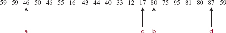
Perhaps the simplest of all sort algorithms is Selection Sort: Given an array x of int values, swap the smallest element with the element at index 0, swap the second smallest element with the element at index 1, and so on.
Example Suppose the array x initially has the usual values, with an arrow pointing to the element at the current index, and the smallest value from that index on in boldface:
The smallest value in the array, 12, is swapped with the value 59 at index 0, and we now have (with the sorted subarray underlined)
Now 16, the smallest of the values from index 1 on, is swapped with the value 46 at index 1:
Then 17, the smallest of the values from index 2 on, is swapped with the value 32 at index 2:
Finally, during the 19th loop iteration, 87 will be swapped with the value 95 at index 18, and the whole array will be sorted:
12 16 17 32 33 40 43 44 46 46 50 55 59 61 75 80 80 81 87 95
In other words, for each value of i between 0 and x.length - 1, the smallest value in the subarray from x [i] to x [x.length −1] is swapped with x [i]. Here is the method definition:
/**
 * Sorts a specified array of int values into ascending order.
 *  The worstTime(n) is O(n * n).
 *
 * @param x - the array to be sorted.
 *
 * @throws NullPointerException - if x is null.
 *
 */
public static void selectionSort (int [ ] x)
{
     // Make x [0 . . .    i] sorted and <= x [i + 1] . . .x [x.length -1]:
     for (int i = 0; i < x.length -1; i++)
     {
           int pos = i;
           for (int k = i + 1; k < x.length; k++)
                 if (x [k] < x [pos])
                         pos = k;
           swap (x, i, pos);
     } // for i
} // method selectionSort
Analysis First, note that the number of loop iterations is independent of the initial arrangement of elements, so worstTime(n) and averageTime(n) will be identical. There are n-1 iterations of the outer loop; when the smallest values are at indexes x[0], x[1],...x[n-2], the largest value will automatically be at index x[n-1]. During the first iteration, with i = 0, there are n-1 iterations of the inner loop. During the second iteration of the outer loop, with i = 1, there are n-2 iterations of the inner loop. The total number of inner-loop iterations is
We conclude that worstTime(n) is quadratic in n. For future reference, note that only n-1 swaps are made.
The worstSpace(n) is constant: only a few variables are needed. But Selection Sort is not stable; see Concept Exercise 11.14.
As we noted in Section 11.2.1, Insertion Sort requires only linear-in-n time if the array is already sorted, or nearly so. That is a clear advantage over Selection Sort, which always takes quadratic-in-n time. In the average case or worst case, Insertion Sort takes quadratic-in-n time, and so a run-time experiment is needed to distinguish between Insertion Sort and Selection Sort. You will get the opportunity to do this in Lab 18.
11.2.3 Bubble Sort
Warning: Do not use this method. Information on Bubble Sort is provided to illustrate a very inefficient algorithm with an appealing name. In this section, you will learn why Bubble Sort should be avoided, so you can illuminate any unfortunate person who has written, used, or even mentioned Bubble Sort.
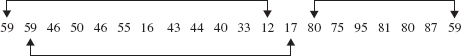
Given an array x of int values, compare each element to the next element in the array, swapping where necessary. At this point, the largest value will be at index x.length −1. Then start back at the beginning, and compare and swap elements. To avoid needless comparisons, go only as far as the last interchange from the previous iteration. Continue until no more swaps can be made: the array will then be sorted.
Example Suppose the array x initially has the following values:
59 46 32 80 46 55 50 43 44 81 12 95 17 80 75 33 40 61 16 87
Because 59 is greater than 46, those two elements are swapped, and we have
46 59 32 80 46 55 50 43 44 81 12 95 17 80 75 33 40 61 16 87
Then 59 and 32 are swapped, 59 and 80 are not swapped, 80 and 46 (at index 4) are swapped, and so on. After the first iteration, x contains
46 32 59 46 55 50 43 44 80 12 81 17 80 75 33 40 61 16 87 95
The last swap during the first iteration was of the elements 95 and 87 at indexes 18 and 19, so in the second iteration, the final comparison will be between the elements at indexes 17 and 18. After the second iteration, the array contains
32 46 46 55 50 43 44 59 12 80 17 80 75 33 40 61 16 81 87 95
The last swap during the second iteration was of the elements 81 and 16 at indexes 16 and 17, so in the third iteration, the final comparison will be between the elements at indexes 15 and 16.
Finally, after 18 iterations, and many swaps, we end up with
12 16 17 32 33 40 43 44 46 46 50 55 59 61 75 80 80 81 87 95
Here is the method definition:
/**
 * Sorts a specified array of int values into ascending order.
 * The worstTime(n) is O(n * n).
 *
 * @param x - the array to be sorted.
 *

 * @throws NullPointerException - if x is null.
 *
 */
public static void bubbleSort (int[ ] x)
{
        int finalSwapPos = x.length - 1,
            swapPos;
        while (finalSwapPos > 0)
        {
              swapPos = 0;
              for (int i = 0; i < finalSwapPos; i++)
                    if (x [i] > x [i + 1])
                    {
                           swap (x, i, i + 1);
                           swapPos = i;
                    } // if
              finalSwapPos = swapPos;
        } // while
 } // method bubbleSort
Analysis If the array starts out in reverse order, then there will be n-1 swaps during the first outer-loop iteration, n-2 swaps during the second outer-loop iteration, and so on. The total number of swaps, and inner-loop iterations, is
We conclude that worstTime(n) is quadratic in n.
What about averageTime(n)? The average number of inner-loop iterations, as you probably would have guessed (!), is
What is clear from the first term in this formula is that averageTime(n) is quadratic in n.
It is not a big deal, but Bubble Sort is very efficient if the array happens to be in order. Then, only n inner-loop iterations (and no swaps) take place. What if the entire array is in order, except that the smallest element happens to be at index x.length −1 ? Then n(n-1)/2 inner-loop iterations still occur!
Swaps take place when, for some index i, the element at index i is greater than the element at index i + 1. This implies that Bubble Sort is stable. And with just a few variables needed (the space for the array was allocated in the calling method), worstSpace(n) is constant.
What drags Bubble Sort down, with respect to run-time performance, is the large number of swaps that occur, even in the average case. You will get first-hand experience with Bubble Sort's run-time sluggishness if you complete Lab 18. As Knuth [1973] says, "In short, the bubble sort seems to have nothing going for it, except a catchy name and the fact that it leads to some interesting theoretical problems."
11.3 The Comparator Interface
Insertion Sort, Selection Sort and Bubble Sort produce an array of int values in ascending order. We could easily modify those methods to sort into descending order. Similarly straightforward changes would allow us to sort arrays of values from other primitive types, such as long or double. What about sorting objects? For objects in a class that implements the Comparable interface, we can sort by the "natural" ordering, as described in Section 10.1.1. For example, here is the heading for a Selection Sort that sorts an array of objects:
/**
 * Sorts a specified array of objects into ascending order.
 * The worstTime(n) is O(n * n).
 *
 * @param x - the array to be sorted.
 *
 * @throws NullPointerException - if x is null.
 *
 */
public static void selectionSort (Object [ ] x)
For the definition of this version, we replace the line
if (x [k] < x [pos])
in the original version with
if (((Comparable)x [k]).compareTo (x [pos]) < 0)
and change heading of the swap method and the type of temp in that method. See Programming Exercise 11.3.
As we saw in Section 10.1.1, the String class implements the Comparable interface with a compareTo method that reflects a lexicographic ordering. If names is an array of String objects, we can sort names into lexicographical order with the call
selectionSort (names);
This raises an interesting question: What if we did not want the "natural" ordering? For example, what if we wanted String objects ordered by the length of the string?
For applications in which the "natural" ordering—through the Comparable interface—is inappropriate, elements can be compared with the Comparator interface. The Comparator interface, with type parameter T (for "type") has a method to compare two elements of type T:
/**
 * Compares two specified elements.
 *
 * @param element1 - one of the specified elements.
 * @param element2 - the other specified element.
 *
 * @return a negative integer, 0, or a positive integer, depending on
 *          whether element1 is less than, equal to, or greater than
 *          element2.

 *
 */
int compare (T element1, T element2);
We can implement the Comparator interface to override the natural ordering. For example, we can implement the Comparator interface with a ByLength class that uses the "natural" ordering for String objects of the same length, and otherwise returns the difference in lengths. Then the 3-character string "yes" is considered greater than the 3-character string "and," but less than the 5-character string "maybe." Here is the declaration of ByLength:
public class ByLength implements Comparator<String>
{
     /**
      * Compares two specified String objects lexicographically if they have the
      * same length, and otherwise returns the difference in their lengths.
      *
      * @param s1 - one of the specified String objects.
      * @param s2 - the other specified String object.
      *
      * @return s1.compareTo (s2) if s1 and s2 have the same length;
      *         otherwise, return s1.length() - s2.length().
      *
      */
     public int compare (String s1, String s2)
     {
            int len1 = s1.length(),
                len2 = s2.length();
            if (len1 == len2)
                     return s1.compareTo (s2);
            return len1 - len2;
     } // method compare
} // class ByLength
One advantage to using a Comparator object is that no changes need be made to the element class: the compare method's parameters are the two elements to be ordered. Leaving the element class unchanged is especially valuable when, as with the String class, users are prohibited from modifying the class.
Here is a definition of Selection Sort, which sorts an array of objects according to a comparator that compares any two objects:
/**
 * Sorts a specified array into the order specified by a specified Comparator
 * object.
 * The worstTime(n) is O(n * n).
 *
 * @param x - the array to be sorted.
 * @param comp - the Comparator object used for ordering.
 *
 * @throws NullPointerException - if x and/or comp is null.
 *
 */

public static void selectionSort (T [ ] x, Comparator comp)
{
      // Make x [0 . . .   i] sorted and <= x [i + 1] . . .x [x.length -1]:
      for (int i = 0; i < x.length -1; i++)
      {
             int pos = i;
             for (int k = i + 1; k < x.length; k++)
                   if (comp.compare (x [k], x [pos]) < 0)
                         pos = k;
             swap (x, i, pos);
      } // for i
} // method selectionSort
The corresponding swap method is:
public static void swap (Object[ ] x, int a, int b)
{
      Object temp = x [a];
      x [a] = x [b];
      x [b] = temp;
} // swap
To complete the picture, here is a small program method that applies this version of selectionSort (note that the enhanced for statement also works for arrays):
import java.util.*; // for the Comparator interface

public class SelectionSortExample
{
      public static void main(String[] args)
      {
            new SelectionSortExample().run();
      } // method main


      public void run()
      {
            String[ ] words = {"Jayden", "Jack", "Rowan", "Brooke"};

            selectionSort (words, new ByLength());
            for (String s : words)
                  System.out.print (s + " ");
            } // method run


} // class SelectionSortExample
The output will be
Jack Rowan Brooke Jayden
The material in this section will be helpful in Section 11.4.1, where we will encounter one of the sort methods in the Java Collections Framework. For this method, called Merge Sort, the element type cannot be primitive; it must be (reference to) Object, or subclass of Object. The method comes in four flavors: the collection to be sorted can be either an array object or a List object, and the ordering may be according to the Comparable interface or the Comparator interface. And Chapter 13 has a sort method with similar flexibility.
In Section 11.4, we consider two important questions: For comparison-based sorts, is there a lower bound for worstTime(n)? Is there a lower bound for averageTime(n)?
11.4 How Fast Can we Sort?
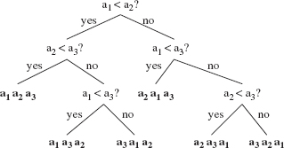
If we apply Insertion Sort, Selection Sort or (perish the thought) Bubble Sort, worstTime(n)and averageTime(n) are quadratic in n. Before we look at some faster sorts, let's see how much of an improvement is possible. The tool we will use for this analysis is the decision tree. Given n elements to be sorted, a decision tree is a binary tree in which each non-leaf represents a comparison between two elements and each leaf represents a sorted sequence of the n elements. For example, Figure 11.1 shows a decision tree for applying Insertion Sort in which the elements to be sorted are stored in the variables a1, a2, and a3:
A decision tree must have one leaf for each permutation of the elements to be sorted2. The total number of permutations of n elements is n!, so if we are sorting n elements, the corresponding decision tree must have n! leaves. According to the Binary Tree Theorem, the number of leaves in any non-empty binary tree t is <= 2height(t). Thus, for a decision tree t that sorts n elements,
n! <= 2height(t)
Taking logs, we get
height(t) >= log2(n!)
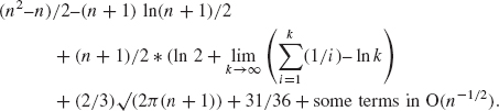
In other words, for any comparison-based sort, there must be a leaf whose depth is at least log2(n!). In the context of decision trees, that means that there must be an arrangement of elements whose sorting requires at least log2(n!) comparisons. That is, worstTime(n) >= log2(n!). According to Concept Exercise 11.7, log2(n!) <= n/2log2(n/2), which makes n/2log2(n/2) a lower bound of worstTime(n)forany comparison-based sort. According to the material on lower bounds from Chapter 3, n/2log2(n/2) is Ω(n log n). So we can say, crudely, that n log n is a lower bound for worstTime(n). Formally, we have
FIGURE 11.1 A decision tree for sorting 3 elements by Insertion Sort
What does Sorting Fact 1 say about upper bounds? We can say, for example, that for any comparison-based sort, worstTime(n) is not O(n). But can we say that for any comparison-based sort, worstTime(n) is O(n log n)? No, because for each of the sorts in Section 11.2, worstTime(n) is O(n2). We cannot even be sure, at this point, that there are any comparison-based sorts whose worstTime(n)is O(n log n). Fortunately, this is not some lofty, unattainable goal. For the comparison-based sort algorithms in Sections 11.4.1 and 13.4, worstTime(n) is O(n log n). When we combine that upper bound with the lower bound from Sorting Fact 1, we will have several sort methods whose worstTime(n) is linear-logarithmic in n.
What about averageTime(n)? For any comparison-based sort, n log n is a lower bound of averageTime(n) as well. To obtain this result, suppose t is a decision tree for sorting n elements. Then t has n! leaves. The average, over all n! permutations, number of comparisons to sort the n elements is the total number of comparisons divided by n!. In a decision tree, the total number of comparisons is the sum of the lengths of all paths from the root to the leaves. This sum is the external path length of the decision tree. By the External Path Length Theorem in Chapter 9, E(t) >= (n !/2) floor (log2(n!)). So we get, for any positive integer n:
averageTime(n)>= average number of comparisons
= E(t)/n!
>= (n !/2)floor(log2(n!))/n!
= (1/2)floor(log2(n!))
>= (1/4)log2(n!)
>= (n/8)log2(n/2) [by Concept Exercise 11.7]
We conclude that n log n is a lower bound of averageTime(n). That is,
Sorting Fact 2:
For comparison-based sorts, averageTime(n) is Ω(n log n).
We noted that there are several sort methods whose worstTime(n) is linear-logarithmic in n. We can use that fact to show that their averageTime(n) must also be linear-logarithmic in n. Why? Suppose we have a sort algorithm for which worstTime(n) is linear-logarithmic in n. That is, crudely, n log n is both an upper bound and a lower bound of worstTime(n). But averageTime(n) <= worstTime(n), so if n log n is an upper bound of worstTime(n), n log n must also be an upper bound of averageTime(n). According to Sorting Fact 2, n log n is a lower bound on averageTime(n). Since n log n is both an upper bound and a lower bound of averageTime(n), we conclude that averageTime(n) must be linear-logarithmic in n. That is,
Sorting Fact 3:
For comparison-based sorts, if worstTime(n) is linear-logarithmic in n, then averageTime(n) must be linear-logarithmic in n.
In Sections 11.4.1 and 11.4.3, we will study two sort algorithms, Merge Sort and Quick Sort, whose averageTime(n) is linear-logarithmic in n. For Merge Sort, worstTime(n) is also linear-logarithmic in n, while for Quick Sort, worstTime(n) is quadratic in n. Strangely enough, Quick Sort is generally considered the most efficient all-around sort. Quick Sort's worst-case performance is bad, but for average-case, runtime speed, Quick Sort is the best of the lot.
11.4.1 Merge Sort
The Merge Sort algorithm, in the Arrays class of the package java.util, sorts a collection of objects. We start with two simplifying assumptions, which we will then dispose of. First, we assume the objects to be sorted are in an array. Second, we assume the ordering is to be accomplished through the Comparable interface.
The basic idea is to keep splitting the n-element array in two until, at some step, each of the subarrays has size less than 7 (the choice of 7 is based on run-time experiments, see Bentley [1993]). Insertion Sort is then applied to each of two, small-sized subarrays, and the two, sorted subarrays are merged together into a sorted, double-sized subarray. Eventually, that subarray is merged with another sorted, double-sized subarray to produce a sorted, quadruple-sized subarray. This process continues until, finally, two sorted subarrays of size n/2 are merged back into the original array, now sorted, of size n.
Here is the method specification for Merge Sort:
/**
 * Sorts a specified array of objects according to the compareTo method
 * in the specified class of elements.
 * The worstTime(n) is O(n log n).
 *
 * @param a - the array of objects to be sorted.
 *
 */
public static void sort (Object[ ] a)
This method has the identifier sort because it is the only method in the Arrays class of the package java.util for sorting an array of objects according to the Comparable interface. Later in this chapter we will encounter a different sort method—also with the identifier sort—for sorting an array of values from a primitive type. The distinction is easy to make from the context, namely, whether the argument is an array of objects or an array from a primitive type such as int or double.
Example To start with a small example of Merge Sort, here are the int values in an array of Integer objects:
59 46 32 80 46 55 87 43 44 81
We use an auxiliary array, aux. We first clone the parameter a into aux. (Cloning is acceptable here because an array object cannot invoke a copy constructor.) We now have two arrays with (separate references to) identical elements. The recursive method mergeSort is then called to sort the elements in aux back into a. Here is the definition of the sort method:
public static void sort (Object[ ] a)
{
       Object aux[ ] = (Object [ ])a.clone();
       mergeSort (aux, a, 0, a.length);
} // method sort
The method specification for mergeSort is
/**
 * Sorts, by the Comparable interface, a specified range of a specified array
 * into the same range of another specified array.
 * The worstTime(k) is O(k log k), where k is the size of the subarray.
 *
 * @param src - the specified array whose elements are to be sorted into another
 *        specified array.
 * @param dest - the specified array whose subarray is to be sorted.
 * @param low - the smallest index in the range to be sorted.
 * @param high - 1 + the largest index in the range to be sorted.
 *
 */
private static void mergeSort (Object src[ ], Object dest[ ], int low, int high)
The reason we have two arrays is to make it easier to merge two sorted subarrays into a larger subarray. The reason for the int parameters low and high is that their values will change when the recursive calls are made. Note that high's value is one greater than the largest index of the subarray being mergeSorted.3
When the initial call to mergeSort is made with the example data, Insertion Sort is not performed because high – low > = 7. (The number 7 was chosen based on run-time experiments.) Instead, two recursive calls are made:
mergeSort (a, aux, 0, 5);
mergeSort (a, aux, 5, 10);
When the first of these calls is executed, high -low = 5 - 0 < 7, so Insertion Sort is performed on the first five elements of aux:
a [0 . . .    4] = {59, 46, 32, 80, 46}

aux [0 . . .   4] = {32, 46, 46, 59, 80}
In general, the two arrays will be identical until an Insertion Sort is performed. When the second recursive call is made, high -low = 10-5, so Insertion Sort is performed on the second five elements of aux:
a [5 . . .    9] = {55, 87, 43, 44, 81}

aux [5 . . .   9] = {43, 44, 55, 81, 87}
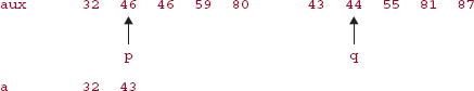
Upon the completion of these two calls to mergeSort, the ten elements of aux, in two sorted subarrays of size 5, are merged back into a, and we are done. The merging is accomplished with the aid of two indexes, p and q. In this example, p starts out as 0 (the low index of the left subarray of aux)and q starts out as 5 (the low index of the right subarray of aux). In the following figure, arrows point from p and q to the elements at aux [p] and aux [q]:
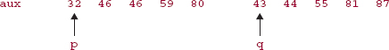
The smaller of aux [p] and aux [q] is copied to a [p] and then the index, either p or q, of that smaller element is incremented:
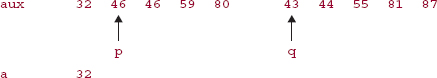
The process is repeated: the smaller of aux [p] and aux [q] is copied to the next location in the array a, and then the index, either p or q, of that smaller element is incremented:
The next three iterations will copy 44, 46, and 46 into a. The process continues until all of the elements from both subarrays have been copied into a. Since each iteration copies one element to a, merging two subarrays of the same size requires exactly twice as many iterations as the size of either subarray. In general, to merge n/k subarrays, each of size k, requires exactly n iterations.
Figure 11.2 summarizes the sorting the above array of ten elements.
FIGURE 11.2 The effect of a call to mergeSort on an array of 10 elements
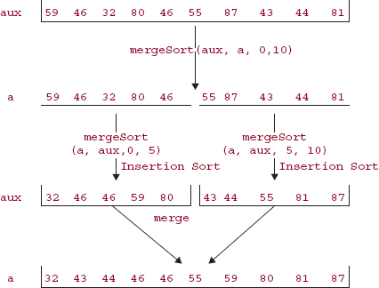
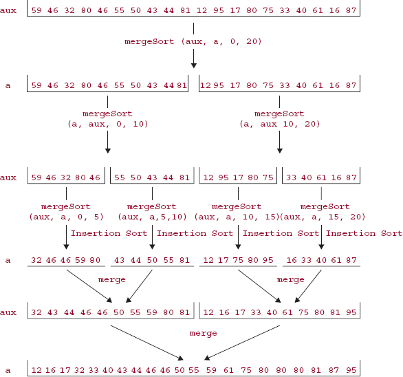
Figure 11.3 incorporates the above example in merge sorting an array of 20 elements. Two pairs of recursive calls are required to merge sort 20 elements.
The successive calls to mergeSort resemble a ping-pong match:
FIGURE 11.3 The effect of a call to mergeSort on an array of 20 elements
The original call, from within the sort method, is always of the form
mergeSort(aux,a, . . .);
So after all of the recursive calls have been executed, the sorted result ends up in a. After the Insertion Sorting has been completed for the two successive subarrays in the recursive call to mergeSort, a merge of those sorted subarrays is performed, and that completes a recursive call to mergeSort.
Here is the complete mergeSort method, including an optimization (starting with //If left subarray ...) that you can safely ignore.
/**
 *  Sorts,  by the Comparable interface,  a specified range of a specified array
 *  into the same range of another specified array.
 *  The worstTime(k) is O(k log k),  where k is the size of the subarray.
 *
 *  @param src - the specified array whose range is to be sorted into another
 *         specified array.

 * @param dest - the specified array whose subarray is to be sorted.
 * @param low: the smallest index in the range to be sorted.
 * @param high: 1 + the largest index in the range to be sorted.
 *
 */
private static void mergeSort (Object src[ ], Object dest[ ], int low, int high)
{
    int length = high - low;


    // Use Insertion Sort for small subarrays.
    if (length < INSERTIONSORT_THRESHOLD /* = 7*/)
    {
    for (int i = low; i < high; i++)
               for (int j = i; j >low && ((Comparable)dest[j - 1])
                                          .compareTo(dest[j]) > 0; j--)
                      swap (dest, j, j-1);
         return
    } // if length < 7

    // Sort left and right halves of src into dest.
    int mid = (low + high) >> 1;   // >> 1 has same effect as / 2, but is faster
    mergeSort (dest, src, low, mid);
    mergeSort (dest, src, mid, high);

    // If left subarray less than right subarray, copy src to dest.
    if (((Comparable)src [mid-1]).compareTo (src [mid]) <= 0)
    {
         System.arraycopy (src, low, dest, low, length);
         return;
    }

    // Merge sorted subarrays in src into dest.
    for (int i = low, p = low, q = mid; i < high; i++)
         if (q>=high ||   (p<mid && ((Comparable)src[p]).compareTo (src[q])<= 0))
                dest [i] = src [p++];
         else
                dest[i] = src[q++];
} // method mergeSort
Analysis We want to get an upper bound on worstTime(n), where n is the number of elements to be sorted. There are four phases: cloning, calls to mergeSort, Insertion Sorting, and merging.
The cloning requires n iterations.
Let L (for "levels") be the number of pairs of recursive calls to mergeSort. The initial splitting into subarrays requires approximately L statements (that is, L pairs of recursive calls). L is equal to the number of times that n is divided by 2. By the Splitting Rule from Chapter 3, the number of times that n can be divided by 2 until n equals 1 is log2 n. But when the size of a subarray is less than 7, we stop dividing by 2. So L is approximately log2(n/6).
For the Insertion Sort phase, we have fewer than n subarrays, each of size less than 7. The maximum number of iterations executed when Insertion Sort is applied to each one of these subarrays is less than 36 because Insertion Sort's worst time is quadratic in the number of elements. So the total number of iterations for this phase is less than 36n.
Finally, the merging back into double-sized subarrays takes, approximately, L times the number of iterations per level, that is, log2(n/6) times the number of iterations executed at any level. At any level, exactly n elements are copied from a to aux (or from aux to a). So the total number of iterations is, approximately, n log2(n/6).
The total number of iterations is less than
n + log2(n/6) + 36n + log2(n/6) * n
From this we conclude that worstTime(n) is less than
n + log2 (n/6) + 36n + n log2(n/6).
That is, worstTime(n) is O(n log n). By Sorting Fact 1 in Section 13.3, for any comparison-based sort, worstTime(n)is Ω(n log n). Since n log n is both an upper bound and a lower bound of worstTime(n), worstTime(n) must be linear-logarithmic in n (that is, Θ(n log n): Big Theta of n log n) That implies, by Sorting Fact 3, that averageTime(n) is also linear-logarithmic in n.
Not only is mergeSort as good as you can get in terms of estimates of worstTime(n) and averageTime(n), but the actual number of comparisons made is close to the theoretical minimum (see Kruse [1987], pages 251-254).
What is worstSpace(n)? The temporary array aux, of size n, is created before mergeSort is called. During the execution of mergeSort, activation records are created at each level. At the first level, two activation records are created; at the second level, four activation records are created; and so on. The total number of activation records created is
(The result on the sum of powers of 2 is from Exercise A2.6 in Appendix 2). Since L ~ log2(n/7), and
2log2n = n
we conclude that the total number of activation records created is linear in n. When we add up the linear-in-n space for aux and the linear-in-n space for activation records, we conclude that worstSpace(n) is linear in n.
Both the Insertion Sorting phase and the merging phase preserve the relative order of elements. That is, mergeSort is a stable sort.
11.4.1.1 Other Merge Sort Methods
The Arrays class also has a version of Merge Sort that takes a Comparator parameter:
public static void sort (T [ ], Comparator<? super T> c)
The essential difference between this version and the Comparable version is that an expression such as
(Comparable)dest[j-1]).compareTo(dest[j])>0
is replaced with
c.compare(dest[j-1], dest[j])>0
For example, suppose words is an array of String objects. To perform Merge Sort on words by the lengths of the strings (but lexicographically for equal-length strings), we utilize the ByLength class from Section 11.3:
Arrays.sort (words, new ByLength());
The Collections class, also in the package java.util, has two versions—depending on whether or not a comparator is supplied—of a Merge Sort method. Each version has a List parameter and starts by copying the list to an array. Then the appropriate version of sort from the Arrays class is called. Finally, during an iteration of the list, each element is assigned the value of the corresponding element in the array. Here, for example, is the Comparator version:
/**
 * Sorts a specified List object of elements from class E according to a
 * specified Comparator object.
 * The worstTime(n) is O(n log n).
 *
 * @param list - the List object to be sorted.
 * @param c - the Comparator object that determines the ordering of elements.
 *
 */
public static void sort (List list, Comparator<? super T> c)
{
     Object a[ ] = list.toArray();
     Arrays.sort(a, c);
     ListIterator i = list.listIterator();
     for (int j=0; j<a.length; j++)
     {
           i.next();
           i.set(a[j]);
     } // for
} // method sort
Both versions of Merge Sort in the Collections class work for any class that implements the List interface, such as ArrayList and LinkedList. The run-time will be somewhat slower than for the Arrays -class versions because of the copying from the list to the array before sorting and the copying from the array to the list after sorting.
One limitation to the current versions of Merge Sort is that they do not allow an array of primitives to be merge sorted. The effect of this restriction can be overcome by merge sorting the corresponding array of objects. For example, to Merge Sort an array of int values, create an array of Integer objects, convert each int value to the corresponding Integer object, apply Merge Sort to the array of Integer objects, then convert the Integer array back to an array of int values. But this roundabout approach will increase the run time for merge sorting.
11.4.2 The Divide-and-Conquer Design Pattern
The mergeSort method is an example of the Divide-and-Conquer design pattern. Every divide-and-conquer algorithm has the following characteristics:
- the method consists of at least two recursive calls to the method itself;
- the recursive calls are independent and can be executed in parallel;
- the original task is accomplished by combining the effects of the recursive calls.
In the case of mergeSort, the sorting of the left and right subarrays can be done separately, and then the left and right subarrays are merged, so the requirements of a divide-and-conquer algorithm are met.
How does a divide-and-conquer algorithm differ from an arbitrary recursive algorithm that includes two recursive calls? The difference is that, for an arbitrary recursive algorithm, the recursive calls need not be independent. For example, in the Towers of Hanoi problem, n-1 disks had to be moved from the source to the temporary pole before the same n-1 disks could be moved from the temporary pole to the destination. Note that the original Fibonacci method from Lab 7 was a divide-and-conquer algorithm, but the fact that the two method calls were independent was an indication of the method's gross inefficiency.
Section 11.4.3 has another example of the divide-and-conquer design pattern.
11.4.3 Quick Sort
One of the most efficient and, therefore, widely used sorting algorithms is Quick sort, developed by C.A.R. Hoare [1962]. The generic algorithm sort is a Quick Sort algorithm based on "Engineering a Sort Function" (see Bentley [1993]). In the Arrays class, Quick Sort refers to any method named sort whose parameter is an array of primitive values, and Merge Sort refers to any method named sort whose parameter is an array of objects.
There are seven versions4 of Quick Sort in the Arrays class: one for each primitive type (int, byte, short, long, char, double, and float) except boolean. The seven versions are identical, except for the specific type information; there is no code re-use. We will illustrate Quick Sort on the int version and, for simplicity, assume that the entire array is to be sorted. The actual code, somewhat harder to follow, allows a specified subarray to be sorted. Here is the (simplified) method specification and definition:
/**
 * Sorts a specified array of int values into ascending order.
 * The worstTime(n) is O(n * n), and averageTime(n) is O(n log n).
 *
 * @param a - the array to be sorted.
 *
 */
public static void sort (int[ ] a)
{
     sort1(a, 0, a.length);
} // method sort
The private sort1 method has the following method specification:
/**
 * Sorts into ascending order the subarray of a specified array, given
 * an initial index and subarray length.
 * The worstTime(n) is O(n * n) and averageTime(n) is O(n log n),

 * where n is the length of the subarray to be sorted.
 *
 * @param x - the array whose subarray is to be sorted.
 * @param off - the start index in x of the subarray to be sorted.
 * @param len - the length of the subarray to be sorted.
 *
 */
private static void sort1(int x[ ], int off, int len)
The basic idea behind the sort1 method is this: we first partition the array x into a left subarray and a right subarray so that each element in the left subarray is less than or equal to each element in the right subarray. The sizes of the subarrays need not be the same. We then Quick Sort the left and right subarrays, and we are done. Since this last statement is easily accomplished with two recursive calls to sort1, we will concentrate on the partitioning phase.
Let's start with the essentials; in Section 11.4.3.1, we'll look at some of the finer points. The first task in partitioning is to choose an element, called the pivot, that each element in x will be compared to. Elements less than the pivot will end up in the left subarray, and elements greater than the pivot will end up in the right subarray. Elements equal to the pivot may end up in either subarray.
What makes Quick Sort fast? With other sorts, it may take many comparisons to put an element in the general area where is belongs. But with Quick Sort, a partition can move many elements close to where they will finally end up. This assumes that the value of the pivot is close to the median5 of the elements to be partitioned. We could, of course, sort the elements to be partitioned and then select the median as the pivot. But that begs the question of how we are going to sort the elements in the first place.
How about choosing x [off] —the element at the start index of the subarray to be sorted—as the pivot? If the elements happen to be in order (a common occurrence), that would be a bad choice. Why? Because the left subarray would be empty after partitioning, so the partitioning would reduce the size of the array to be sorted by only one. Another option is to choose x [off + len/2] as the pivot, that is, the element in the middle position. If the range happens to be in order, that is the perfect choice; otherwise, it is as good a blind choice as any other.
With a little extra work, we can substantially increase the likelihood that the pivot will split the range into two subarrays of approximately equal size. The pivot is chosen as the median of the elements at indexes off, off + len/2, and off + len −1. The median of those three elements is taken as a simply calculated estimate of the median of the whole range.
Before looking at any more details, let's go through an example.
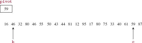
Example We start with the usual sample of twenty values given earlier:
59 46 32 80 46 55 50 43 44 81 12 95 17 80 75 33 40 61 16 87
In this case, we choose the median of the three int values at indexes 0, 10, and 19. The median of 59, 12, and 87 is 59, so that is the original pivot.
We now want to move to the left subarray all the elements that are less than 59 and move to the right subarray all the elements that are greater than 59. Elements with a value of 59 may end up in either subarray, and the two subarrays need not have the same size.
To accomplish this partitioning, we create two counters: b, which starts at off and moves upward, and c, which starts at off + len - 1 and moves downward. There is an outer loop that contains two inner loops. The first of these inner loops increments b until x [b] >= pivot. Then the second inner loop decrements c until x [c] <= pivot. If b is still less than or equal to c when this second inner loop terminates, x [b] and x [c] are swapped, b is incremented, c is decremented, and the outer loop is executed again. Otherwise, the outer loop terminates.
The reason we loop until x [b] >= pivot instead of x [b] > pivot is that there might not be any element whose value is greater than the pivot. In Section 11.4.3.1, we'll see a slightly different loop condition to avoid stopping at, and therefore swapping, the pivot.
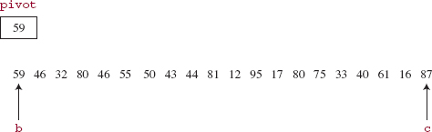
For the usual sample of values, pivot has the value 59, b starts at 0 and c starts at 19. In Figure 11.4, arrows point from an index to the corresponding element in the array:
FIGURE 11.4 The start of partitioning
The first inner loop terminates immediately because x [b] = 59 and 59 is the pivot. The second inner loop terminates when c is decremented to index 18 because at that point, x [c] = 16 < 59. When 59 and 16 are swapped and b and c are bumped, we get the situation shown in Figure 11.5.
FIGURE 11.5 The state of partitioning after the first iteration of the outer loop
Now b is incremented twice more, and at that point we have x [b] = 80 > 59. Then c is decremented once more, to where x [c] = 40 < 59. After swapping x [b] with x [c] and bumping b and c, we have the state shown in Figure 11.6.
During the next iteration of the outer loop, b is incremented five more times, c is not decremented, 81 and 33 are swapped, then the two counters are bumped, and we have the state shown in Figure 11.7.
FIGURE 11.6 The state of partitioning after the second iteration of the outer loop
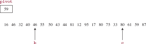
FIGURE 11.7 The state of partitioning after the third iteration of the outer loop
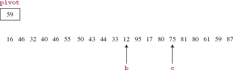
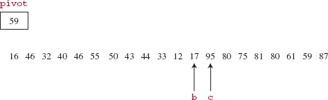
During the next iteration of the outer loop, b is incremented once (x [b] = 95), and c is decremented twice (x [c] = 17). Then 95 and 17 are swapped, and b and c are bumped. See Figure 11.8.
All of the elements in the subarray at indexes 0 through c are less than or equal to the pivot, and all the elements in the subarray at indexes b through 19 are greater than or equal to the pivot.
We finish up by making two recursive calls to sort1:
sort1 (x, off, c + 1 - off);            // for this example, sort1 (x, 0, 12);
sort1 (x, b, off + len -b);             // for this example, sort1 (x, 12, 8);
In this example, the call to sort1 (x, off, c + 1 - off) will choose a new pivot, partition the subarray of 12 elements starting at index 0, and make two calls to sort1. After those two calls (and their recursive calls) are completed, the call to sort1 (x, b, off + len -b) will choose a new pivot, and so on. If we view each pair of recursive calls as the left and right child of the parent call, the execution of the calls in the corresponding binary tree follows a preOrder traversal: the original call, then the left child of that call, then the left child of that call, and so on. This leftward chain stops when the subarray to be sorted has fewer than two elements.
FIGURE 11.8 The state of partitioning after the outer loop is exited
After partitioning, the left subarray consists of the elements from indexes off through c, and the right subarray consists of the elements from indexes b through off + len −1. The pivot need not end up in either subarray. For example, suppose at some point in sorting, the subarray to be partitioned contains
15 45 81
The pivot, at index 1, is 45, and both b and c move to that index in searching for an element greater than or equal to the pivot and less than or equal to the pivot, respectively. Then (wastefully) x [b] is swapped with x [c], b is incremented to 2, and c is decremented to 0. The outer loop terminates, and no further recursive calls are made because the left subarray consists of 15 alone, and the right subarray consists of 81 alone. The pivot is, and remains, where it belongs.
Similarly, one of the subarrays may be empty after a partitioning. For example, if subarray to be partitioned is
15 45
The pivot is 45, both b and c move to that index, 45 is swapped with itself, b is incremented to 2 and c is decremented to 0. The left subarray consists of 15 alone, the pivot is in neither subarray, and the right subarray is empty.
Here is the method definition for the above-described version of sort1 (the version in the Arrays class has a few optimizations, discussed in Section 11.4.3.1):
/**
 * Sorts into ascending order the subarray of a specified array, given
 * an initial index and subarray length.
 * The worstTime(k) is O(n * n) and averageTime(n) is O(n log n),
 * where n is the length of the subarray to be sorted.
 *
 * @param x - the array whose subarray is to be sorted.
 * @param off - the start index in x of the subarray to be sorted.
 * @param len - the length of the subarray to be sorted.
 *
 */
private static void sort1(int x[ ], int off, int len)
{
      // Choose a pivot element, v
      int m = off + (len >> 1),
          l = off,
          n = off + len - 1;

      m = med3 (x, l, m, n); // median of 3
      int v = x [m];   // v is the pivot

      int b = off,
          c = off + len - 1;
      while(true)
      {
              while (b <= c && x [b] < v)
                   b++;
              while (c >= b && x [c] > v)
                   c--;

              if (b > c)
                   break ;
              swap (x, b++, c--);
      } // while true


      if (c + 1 -off > 1)
              sort1 (x, off, c + 1 -off);
      if (off + len -b > 1)
              sort1 (x, b, off + len -b);
} // method sort1

/**
 * Finds the median of three specified elements in a given array..
 *
 * @param x - the given array.
 * @param a - the index of the first element.
 * @param b - the index of the second element.
 * @param c - the index of the third element
 *
 * @return the median of x [a], x [b], and x [c].
 *
 */
private static int med3(int x[], int a, int b, int c) {
     return (x[a] < x[b] ?
            (x[b] < x[c] ? b : x[a] < x[c] ? c : a) :
            (x[b] > x[c] ? b : x[a] > x[c] ? c : a));
} // method med3

/**
 * Swaps two specified elements in a specified array.
 *
 * @param x - the array in which the two elements are to be swapped.
 * @param a - the index of one of the elements to be swapped.
 * @param b - the index of the other element to be swapped.
 *
 */
private static void swap(int x[], int a, int b) {
     int t = x[a];
     x[a] = x[b];
     x[b] = t;
} // method swap
Analysis We can view the effect of sort1 as creating an imaginary binary search tree, whose root element is the pivot and whose left and right subtrees are the left and right subarrays. For example, suppose we call Quick Sort for the following array of 15 integers
68 63 59 77 98 87 84 51 17 12 8 25 42 35 31
FIGURE 11.9 The imaginary binary search tree created by repeated partitions, into equal sized subarrays, of the array [68 63 59 77 98 87 84 51 17 12 8 25 42 35 31]
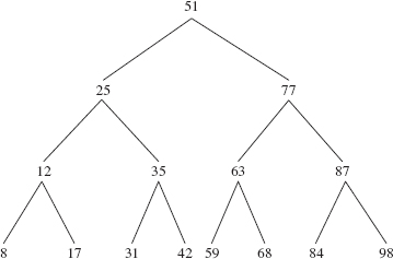
The first pivot chosen is 51; after the first partitioning, the pivot of the left subarray is 25 and the pivot of the right subarray is 77. Figure 11.9 shows the full binary-search-tree induced during the sorting of the given array. In general, we get a full binary search tree when each partition splits its subarray into two subarrays that have the same size. We would also get such a tree if, for example, the elements were originally in order or in reverse order, because then the pivot would always be the element at index off + len/2, and that element would always be the actual median of the whole sequence.
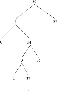
Contrast the above tree with the tree shown in Figure 11.10. The tree in Figure 11.10 represents the partitioning generated, for example, by the following sequence of 38 elements (the pivot is the median of 1, 37, and 36):
1, 2,3,.. .,17,18, 0,37,19, 20,21,..,35,36
The worst case will occur when, during each partition, the pivot is either the next-to-smallest or next-to-largest element. That is what happens for the sequence that generated the tree in Figure 11.10.
For any array to be sorted, the induced binary search tree can help to determine how many comparisons are made in sorting the tree. At level 0, each element is compared to the original pivot, for a total of approximately n loop iterations (there will be an extra iteration just before the counters cross). At level 1, there are two subarrays, and each element in each subarray is compared to its pivot, for a total of about n iterations. In general, there will be about n iterations at each level, and so the total number of iterations will be, approximately, n times the number of levels in the tree.
We can now estimate the average time for the method sort1. The average is taken over all n! initial arrangements of elements in the array. At each level in the binary search tree that represents the partitioning, about n iterations are required. The number of levels is the average height of that binary search tree. Since the average height of a binary search tree is logarithmic in n, we conclude that the total number of iterations is linear-logarithmic in n. That is, averageTime(n) is linear-logarithmic in n. By Sorting Fact 2 in Section 11.3.1, the averageTime(n) for Quick Sort is optimal.
In the worst case, the first partition requires about n iterations and produces a subarray of size n − 2 (and another subarray of size 1). When this subarray of size n − 2 is partitioned, about n − 2 iterations are required, and a subarray of size n − 4 is produced. This process continues until the last subarray, of size 2 is partitioned. The total number of iterations is approximately n + (n − 2) + (n − 4) + ... + 4 + 2, which is, approximately, n2/4. We conclude that worstTime(n) is quadratic in n.
FIGURE 11.10 Worst-case partitioning: each partition reduces by only 2 the size of the subarray to be Quick Sorted. The corresponding binary search tree has a leaf at every non-root level. The subtrees below 32 are not shown
Quick Sort's space needs are due to the recursive calls, so the space estimates depend on the longest chain of recursive calls, because that determines the maximum number of activation records in the runtime stack. In turn, the longest chain of recursive calls corresponds to the height of the induced binary search tree. In the average case, that height is logarithmic in n, and we conclude that averageSpace(n)is logarithmic in n. In the worst case, that height is linear in n, so worstSpace(n) is linear in n.
Quick Sort is not a stable sort. For example, in the example given at the beginning of this section, there are two copies of 80. The one at index 3 is swapped into index 16, and the one at index 13 remains where it starts.
Quick Sort is another example of the Divide-and-Conquer design pattern. Each of the recursive calls to sort1 can be done in parallel, and the combined effect of those calls is a sorted array.
11.4.3.1 Optimizations to the Quick Sort Algorithm
The Arrays class's sort1 method has several modifications to the definition given in Section 11.4.3. The modifications deal with handling small subarrays, handling large subarrays, and excluding the pivot (and elements equal to the pivot) from either subarray.
The partitioning and Quick Sorting continues only for subarrays whose size is at least 7. For subarrays of size less than 7, Insertion Sort is applied. This avoids using the partitioning and recursive-call machinery for a task that can be handled efficiently by Insertion Sort. The choice of 7 for the pivot is based on empirical tests described in Bentley [1993]. For arrays of size 7, the pivot is chosen as the element at the middle index, that is, pivot = x [off + (len >> 1)]. (Recall that len >> 1 is a fast way to calculate len/2.) For arrays of size 8 through 40, the pivot is chosen—as we did in Section 11.4.3—as the median of the three elements at the first, middle, and last indexes of the subarray to be partitioned.
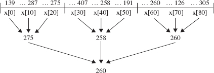
For subarrays of size greater than 40, an extra step is made to increase the likelihood that the pivot will partition the array into subarrays of about the same size. The region to be sorted is divided into three parts, the median-of-three technique is applied to each part, and then the median of those three medians becomes the pivot. For example, if off = 0 and len = 81, Figure 11.11 shows how the pivot would be calculated for a sample arrangement of the array x. These extra comparisons have a price, but they increase the likelihood of an even split during partitioning.
FIGURE 11.11 The calculation of the pivot as the median of three medians. The median of (139, 287, 275) is 275; the median of (407, 258, 191) is 258; the median of (260, 126, 305) is 260. The median of (275, 258, 260) is 260, and that is chosen as the pivot
There are two additional refinements, both related to the pivot. Instead of incrementing b until an element greater than or equal to the pivot is found, the search is given by
while (b <= c && x[b] <= v)
A similar modification is made in the second inner loop. This appears to be an optimization because the pivot won't be swapped, but the inner-loop conditions also test b < = c. That extra test may impede the speed of the loop more than avoiding needless swaps would enhance speed.
That refinement enables another pivot-related refinement. For the sort1 method defined above, the pivot may end up in one of the subarrays and be included in subsequent comparisons. These comparisons can be avoided if, after partitioning, the pivot is always stored where it belongs. Then the left subarray will consist of elements strictly less than the pivot, and the right subarray will consist of elements strictly greater than the pivot. Then the pivot—indeed, all elements equal to the pivot—will be ignored in the rest of the Quick Sorting.
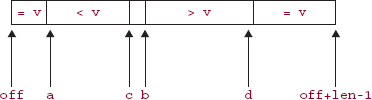
To show you how this can be accomplished, after the execution of the outer loop the relation of segments of the subarray to the pivot v will be as shown in Figure 11.12.
At this point, equal-to-pivot elements are swapped back into the middle of the subarray. The left and right subarrays in the recursive calls do not include the equal-to-pivot elements.
As the partitioning of a subarray proceeds, the equal-to-pivot elements are moved to the beginning and end of the subarray with the help of a couple of additional variables:
int a = off,
d = off + len - 1;
FIGURE 11.12 The relationship of the pivot v to the elements in the subarray to be partitioned. The leftmost segment and rightmost segment consist of copies of the pivot

The index a will be one more than highest index of an equal-to-pivot element in the left subarray, and d will be one less than the lowest index of an equal-to-pivot element in the right subarray. In the first inner loop, if x [b] = v, we call
swap (x, a++, b);
Similarly, in the second inner loop, if x[c]=v, we call
swap (x, c, d-);
Figure 11.13 indicates where indexes a and d would occur in Figure 11.12.
FIGURE 11.13 A refinement of Figure 11.12 to include indexes a and d
For an example that has several copies of the pivot, suppose we started with the following array of 20 ints:
59 46 59 80 46 55 87 43 44 81 95 12 17 80 75 33 40 59 16 50
During partitioning, copies of 59 are moved to the leftmost and rightmost part of the array. After b and c have crossed, we have the arrangement shown in Figure 11.14.
FIGURE 11.14 The status of the indexes a, b, c, and d after partitioning
Now all the duplicates of 59 are swapped into the middle, as shown in Figure 11.15.
FIGURE 11.15 The swapping of equal-to-pivot elements to the middle of the array
We now have the array shown in Figure 11.16:
FIGURE 11.16 The array from Figure 11.15 after the swapping
![]()
The next pair of recursive calls is:
sort1 (x, 0, 11);
sort1 (x, 14, 6);
The duplicates of 59, at indexes 11, 12, and 13, are in their final resting place.
Here, from the Arrays class, is the complete definition (the swap and med3 method definitions were given in Section 11.4.3):
/**
 * Sorts into ascending order the subarray of a specified array, given
 * an initial index and subarray length.
 * The worstTime(n) is O(n * n) and averageTime(n) is O(n log n),
 * where n is the length of the subarray to be sorted.
 *
 * @param x - the array whose subarray is to be sorted.
 * @param off - the start index in x of the subarray to be sorted.
 * @param len - the length of the subarray to be sorted.
 *
 */
private static void sort1(int x[ ], int off, int len)
{

      // Insertion sort on smallest arrays
      if (len < 7) {
         for (int i=off; i<len+off; i++)
            for (int j=i; j>off && x[j-1]>x[j]; j--)
                swap(x, j, j-1);
         return;
      }

      // Choose a partition element, v
      int m = off + (len >> 1);       // Small arrays, middle element
      if (len > 7) {
            int l = off;
            int n = off + len - 1;
            if (len > 40) {        // Big arrays, pseudomedian of 9
               int s = len/8;
               l = med3(x, l,     l+s, l+2*s);
               m = med3(x, m-s,   m,   m+s);
               n = med3(x, n-2*s, n-s, n);
        }
        m = med3(x, l, m, n); // Mid-size, med of 3
      }
      int v = x[m];   // v is the pivot

      // Establish Invariant: = v; < v; > v; = v
      int a = off, b = a, c = off + len - 1, d = c;
      while(true) {
         while (b <= c && x[b] <= v) {
              if (x[b] == v)

                  swap(x, a++, b);
              b++;
         }
         while (c >= b && x[c] >= v) {
              if (x[c] == v)
                  swap(x, c, d--);
              c--;
         }
         if (b > c)
              break;
         swap(x, b++, c--);
      }

      // Swap partition elements back to middle
      int s, n = off + len;
      s = Math.min(a-off, b-a );   vecswap(x, off, b-s, s);
      s = Math.min(d-c,   n-d-1); vecswap(x, b,    n-s, s);

      // Recursively sort non-partition-elements
      if ((s = b-a) > 1)
          sort1(x, off, s);
      if ((s = d-c) > 1)
          sort1(x, n-s, s);
}

/**
 *  Swaps the elements in two specified subarrays of a given array.
 *  The worstTime(n) is O(n), where n is the number of pairs to be swapped.
 *
 *  @param x - the array whose subarrays are to be swapped.
 *  @param a - the start index of the first subarray to be swapped.
 *  @param b - the start index of the second subarray to be swapped.
 *  @param n - the number of elements to be swapped from each subarray.
 *
 */
private static void vecswap(int x[], int a, int b, int n) {
     for (int i=0; i<n; i++, a++, b++)
          swap(x, a, b);
} // method vecswap
With these optimizations, the results of the analysis in Section 11.4.3 still hold. For example, we now show that if Quick Sort is applied to a large array, worstTime(n) will still be quadratic in n. For n> 40, the worst case occurs when the 9 elements involved in the calculation of the median of medians are the five smallest and four largest elements. Then the fifth-smallest element is the best pivot possible, and the partitioning will reduce the size of the subarray by 5. In partitioning the subarray of size n − 5, we may have the four smallest and five largest tested for median of medians, and the size will again be reduced by only 5. Since the number of iterations at each level is, approximately, the size of the subarray to be partitioned, the total number of iterations is, approximately,
n + (n − 5) + (n − 10) + (n − 15) + ... + 45
which is, approximately, n2/10. That is, worstTime(n) is quadratic in n.
For a discussion of how, for any positive integer n, to create an array of int values for which Quick Sort takes quadratic time, see McIlroy [1999].
One debatable issue with the above Quick Sort algorithm is its approach to duplicates of the chosen pivot. The overall algorithm is significantly slowed by the test for equality in the inner loops of sort1. Whether this approach enhances or diminishes efficiency depends on the number of multiple pivot copies in the array.
We finish up this chapter with a sort method that is not comparison-based, and therefore essentially different from the other sort methods we have seen.
11.5 Radix Sort
Radix Sort is unlike the other sorts presented in this chapter. The sorting is based on the internal representation of the elements to be sorted, not on comparisons between elements. For this reason, the restriction that worstTime(n) can be no better than linear-logarithmic in n no longer applies.
Radix Sort was widely used on electromechanical punched-card sorters that appear in old FBI movies. The interested reader may consult Shaffer [1998].
For the sake of simplicity, suppose we want to sort an array of non-negative integers of at most two decimal digits. The representation is in base 10, also referred to as radix 10—this is how Radix Sort gets its name. In addition to the array to be sorted, we also have an array, lists, of 10 linked lists, with one linked list for each of the ten possible digit values.
During the first outer-loop iteration, each element in the array is appended to the linked list corresponding to the units digit (the least-significant digit) of that element. Then, starting at the beginning of each list, the elements in lists [0], lists [1], and so on are stored back in the original array. This overwrites the original array. In the second outer-loop iteration, each element in the array is appended to the linked list corresponding to the element's tens digit. Then, starting at the beginning of each list, the elements in lists [0], lists [1], and so on are stored back in the original array.
Here is the method specification:
/**
 * Sorts a specified array into ascending order.
 * The worstTime(n) is O(n log N), where n is the length of the array, and N
 * is the largest number (in absolute value) of the numbers in the array.
 *
 * @param a - the array to be sorted.
 *
 * @throws NullPointerException - if a is null.
 *
 */
public static void radixSort (int[ ] a)
Example Suppose we start with the following array of 12 int values:
85 3 19 43 20 55 42 91 21 85 73 29
FIGURE 11.17 An array of linked lists after each element in the original array is appended to the linked list that corresponds to the element's units digit
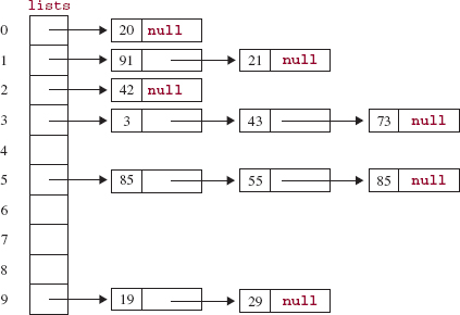
After each of these is appended to the linked list corresponding to its units (that is, rightmost) digit, the array of linked lists will be as shown in Figure 11.17.
Then, starting at the beginning of each list, elements in lists [0], lists [1], and so on are stored back in a. See Figure 11.18.
FIGURE 11.18 The contents of the array a, with the elements ordered by their units digits
![]()
The elements in the array a have now been ordered by their units digits.
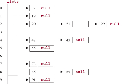
In the next outer-loop iteration, each element in a is appended to the list corresponding to the element's tens digit, as shown in Figure 11.19.
Finally (because the integers had at most two digits), starting at the beginning of each list, the integers in lists [0], lists [1], and so on are stored back in a:
3 19 20 21 29 42 43 55 73 85 85 91
The elements in a have been ordered by their tens digits, and for numbers with the same tens digits, they have been ordered by their units digits. In other words, the array a is sorted.
What happens in general? Suppose we have two integers x and y, with x < y. Here's how Radix Sort ensures that x ends up at a smaller index in the array. If x has fewer digits than y, then in the final iteration of the outer loop, x will be placed in lists [0] and y will be placed in a higher-indexed list because y's leftmost digit is not zero. Then when the lists are stored back in the array, x will be at a smaller index than y.
If x and y have the same number of digits, start at the leftmost digit in each number and, moving to the right, find the first digit in x that is smaller than the corresponding digit in y. (For example, if x = 28734426 and y = 28736843, the thousands digit in x is less than the thousands digit in y.) Then at the start of that iteration of the outer loop, x will be placed in a lower indexed list than y. Then when the lists are stored back in the array, x will be at a smaller index than y. And from that point on, the relative positions of x and y in the array will not change because they agree in all remaining digits.
FIGURE 11.19 The array of linked lists after each element in the array a has been appended to the linked list corresponding to its tens digit
There is a slight difficulty in converting the outline in the previous paragraphs into a Java method definition. The following statement is illegal:
LinkedList<Integer>[ ] lists = new LinkedList<Integer> [10];
The reason is that arrays use covariant subtyping (for example, the array Double[ ] is a subtype of Object[ ]), but parameterized types use invariant subtyping (for example, LinkedList<Double> is not a subtype of LinkedList<object>). We cannot create an array whose elements are parameterized collections. But it is okay to create an array whose elements are raw (that is, unparameterized) collections. So we will create the array with the raw type LinkedList, and then construct the individual linked lists with a parameterized type.
Here is the method definition:
/**
 * Sorts a specified array into ascending order.
 * The worstTime(n) is O(n log N), where n is the length of the array, and N is the largest
 * number (in absolute value) of the numbers in the array.
 *
 * @param a - the array to be sorted.
 *
 */
public static void radixSort (int [ ] a)
{
     final int RADIX = 10;

     int biggest = a [0],
          i;

     for (i = 1; i < a.length; i++)
         if (a [i] > biggest)
             biggest = a [i];

     int maxDigits = (int)Math.floor (Math.log (biggest) / Math.log (10)) + 1;

     long quotient = 1;       // the type is long because the largest number may have
                              // 10 digits; the successive quotients are 1, 10, 100, 1000,
                              // and so on. 10 to the 10th is too large for an int value.

    LinkedList[ ] lists = new LinkedList [RADIX];

    for (int m = 0; m < RADIX; m++)
         lists [m] = new LinkedList<Integer>();

   // Loop once for each digit in the largest number:
   for (int k = 0; k < maxDigits; k++)
   {
      // Store each int in a as an Integer in lists at the index of a [i]-s kth-smallest digit:
      for (i = 0; i < a.length; i++)
           ((LinkedList<Integer>)lists [(int)(a [i] / quotient) % RADIX]).add (a [i]);
      i = 0;

      // Store each Integer in list [0], list [1], . . ., as an int in a:
      for (int j = 0; j < RADIX; j++)
      {
           for (Integer anInt : (LinkedList<Integer>)lists [j])
                 a [i++] = anInt;   // unboxing
           lists [j].clear();
      } // for j
      quotient *= RADIX;
   } // for k
} // method radixSort
Analysis Suppose N is the largest integer in the array. The number of outer-loop iterations must be at least ceil (log10 N), so worstTime(n, N) is O(n log N). If the array also includes negative integers, N is chosen as the largest number in absolute value. Each array element is also stored in a linked list, and so worstSpace(n) is linear in n.
The elements are stored first-in, first-out in each list, and that makes Radix Sort stable.
Note: The elements in this example of Radix Sort are of type int, but with a slight change, the element type could also be String, for example. There would be one list for each possible character in the String class. Because each Unicode character occupies 16-bits, the number of distinct characters is 216 = 65,536 characters. That would require 65,536 linked lists! Instead, the allowable character set would probably be reduced to ASCII, an 8-bit code, so there would be only 28 = 256 characters, and therefore 256 lists.
Lab 18 includes Radix Sort in a run-time experiment on sort methods.
You are now prepared to do Lab 18: Run-times for Sort Methods.
SUMMARY
Table 11.1 provides a thumbnail sketch of the sort algorithms presented in this chapter.
Table 11.1 Important features of sort algorithms from Chapter 11. Run-time rank is based on the time to sort n randomly-generated integers. The restrictions on element type are for the versions of Merge Sort and Quick Sort in the Java Collections Framework (JCF). For Radix Sort, N refers to the largest number in the collection
CROSSWORD PUZZLE
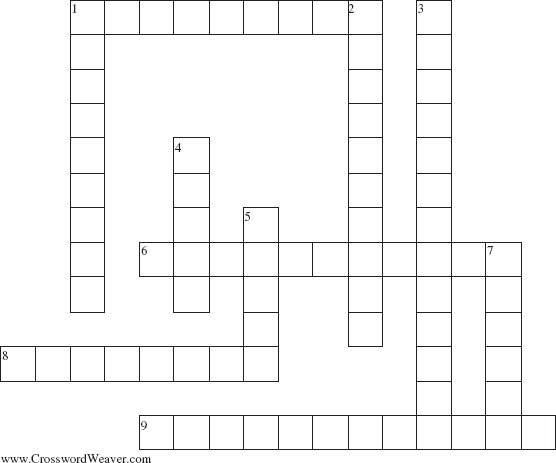
| ACROSS | DOWN |
| 1. The worstTime(n) for the three simple sorts is _______ in n. | 1. The sorting algorithm whose average run-time performance is fastest |
| 6. The class in the Java Collections Framework that has exactly two versions of the Merge Sort algorithm | 2. An interface whose implementation allows "unnatural" comparisons of elements |
| 8. The number of different versions of the Quick Sort algorithm in the Arrays class | 3. The only one of the three simple sorts that is not stable |
| 4. In Quck Sort partitioning, the element that every element in a subarray is compared to | |
| 9. Given n elements to be sorted, a ______ is a binary tree in which each non-leaf represents a comparison between two elements and each leaf represents a sorted sequence of the n elements. | 5. For comparison-based sorts, averageTime(n) is BigOmega (_________). |
| 7. A ______ sort method preserves the relative order of equal elements. |
CONCEPT EXERCISES
11.1 Trace the execution of each of the six sort methods—Insertion Sort, Selection Sort, Bubble Sort, Merge Sort, Quick Sort, and Radix Sort—with the following array of values:
10 90 45 82 71 96 82 50 33 43 67
11.2 a. For each sort method, rearrange the list of values in Concept Exercise 11.1 so that the minimum number of element-comparisons would be required to sort the array.
b. For each sort method, rearrange the list of values in Concept Exercise 11.1 so that the maximum number of element-comparisons would be required to sort the sequence.
11.3 Suppose you want a sort method whose worstTime(n) is linear-logarithmic in n, but requires only linear-in-n time for an already sorted collection. None of the sorts in this chapter have those properties. Create a sort method that does have those properties.
Hint: Add a front end to Merge Sort to see if the collection is already sorted.
11.4 For the optimized Quick Sort in Section 11.4.3.1, find an arrangement of the integers 0 ... 49 for which the first partition will produce a subarray of size 4 and a subarray of size 44. Recall that because the number of values is greater than 40, the pivot is the "super-median," that is, the median of the three median-of-threes.
11.5 a. Suppose we have a sort algorithm whose averageTime(n) is linear-logarithmic in n. For example, either Merge Sort or Quick Sort would qualify as such an algorithm. Let runTime(n) represent the time, in seconds, for the implementation of the algorithm to sort n random integers. Then we can write:
runTime(n) ![]() k(c) * n * logcn seconds,
k(c) * n * logcn seconds,
where c is a an integer variable and k is a function whose value depends on c. Show that runTime(cn) ![]() runTime(n) *(c + c/ logcn).
runTime(n) *(c + c/ logcn).
b. Use the technique in Concept Exercise 11.5.a to estimate runTime(200000) if runTime(100000) = 10.0 seconds.
11.6 Show that seven comparisons are sufficient to sort any collection of five elements.
Hint: Compare the first and second elements. Compare the third and fourth elements. Compare the two larger elements from the earlier comparisons. With three comparisons, we have an ordered chain of three elements, with the fourth element less than (or equal to) one of the elements in the chain. Now compare the fifth element to the middle element in the chain. Complete the sorting in three more comparisons. Note that ceil(log25!) = 7, so some collections of five elements cannot be sorted with 6 comparisons.
11.7 Show that log2 n! >= n/2log2 (n/2) for any positive integer n.
Hint: For any positive integer n,
11.8 Show how Quick Sort's partitioning can be used to develop a method, median, that finds the median of an array of int values. For the method median, averageTime(n) must be linear in n.
Hint: Suppose we want to find the median of x [0... 10000]. Of course, if we Quick Sort the array, the median would be in x [5000], but then averageTime(n) would be linear-logarithmic in n. To get an idea of how to proceed, let's say that the first partition yields a left subarray x [0... 3039] and a right subarray x [3055 ... 10000], with copies of the pivot in x [3040 ... 3054]. Since every int value in the left subarray is less than every int value in the right subarray, which subarray must contain the median? The other subarray can be ignored from then on, so the array is not completely sorted.
11.9 Consider the following, consecutive improvements to Insertion Sort:
- Replace the call to the method swap with in-line code:
public static void insertionSort (int[ ] x)
{
    int temp;

    for (int i = 1; i < x.length; i++)
        for (int k= i; k > 0 && x [k -1] > x [k]; j--)
        {
               temp = x [k];
               x [k] = x [k -1];
               x [k -1] = temp;
        } // inner for
} // method insertionSort
- Notice that in the inner loop in part a, temp is repeatedly assigned the original value of x [i]. For example, suppose the array x has
32 46 59 80 35
and j starts at 4. Then 35 hops its way down the array, from index 4 to index 1. The only relevant assignment from temp is that last one. Instead, we can move the assignments to and from temp out of the inner loop:
int temp,
      k;

for (int i = 1; i < x.length; i++)
{
     temp = x [i];
     for (k = i; k > 0 && x [k -1] > temp; k--)
         x [k] = x [k -1];
         x [k] = temp;
} // outer for
Will these changes affect the estimates for worstTime(n) and averageTime(n)?
11.10 If x is an array, Arrays.sort (x) can be called. Will x be Merge Sorted or Quick Sorted? How is the determination made?
11.11 Show how Merge Sort can be used to sort an array of primitives with the help of the wrapper classes.
11.12 The Java Collection Framework's version of Quick Sort can be applied only to an array of a primitive type, such as int or double. Exactly what would have to be changed to create a Quick Sort method that could be applied to an array of objects?
11.14 If Merge Sort is applied to a collection with 25 elements, what are the values of the index arguments for the first two recursive calls?
11.14 Give an example to show that Selection Sort is not a stable sort.
Hint: you need only three elements.
PROGRAMMING EXERCISES
11.1 For Concept Exercise 11.9, conduct a timing experiment to estimate the run-time effect of the changes made.
11.2 In the Java Collections Framework version of Quick Sort, special care is taken during partitioning to make sure that the pivot, and elements equal to the pivot, are not in either of the subarrays created. Estimate—in percentage terms—how much faster Quick Sort would run, on average, if this special care were not taken. Conduct a timing experiment to test your hypothesis.
11.3 In the med3 method, replace the two applications of the conditional operator with if statements.
11.5 For the original version of Quick Sort in Section 11.4.3, replace the inner-loop conditions from
while (x [b] < v) and while (x [c] > v)
to
while (b <= c && x [b] <= v) and while (c >= b && x [c] >= v)
Create a small program method to apply this version of Quick Sort to the following array of int values:
46 59
Explain the results.
11.5 Develop a version of Radix Sort to sort an array of String objects. You may assume that each String object contains only ASCII characters, and that the maximum size of any String object is 30. Use JUnit to test your radixSort method.
Hint: Instead of the quotient variable, use the charAt method in the String class.
11.6 Modify the radixSort method in Section 11.5 to use an ArrayList instead of an array.
Hint: Start with
ArrayList<LinkedList<Integer>> lists = new ArrayList<LinkedList<Integer>>(RADIX);
Then append 10 empty linked lists to lists.
Programming Project 11.1: Sorting a File into Ascending Order
Analysis The input line will contain the path to the file to be sorted. Each element in the file will consist of a name—last name followed by a blank followed by first name followed by a blank followed by middle name—and social security number. The file is to be sorted by name; equal names should be ordered by social security number. For example, after sorting, part of the file might be as follows:
| Jones Jennifer Mary | 222222222 |
| Jones Jennifer Mary | 644644644 |
For convenience, you may assume that each name will have a middle name. Suppose the file persons.dat consists of the following:
System Test 1:
Please enter the path for the file to be sorted.
persons.dat
The file persons.dat has been sorted.
The file persons.dat will now consist of
| Deusenbery Amanda May | 777777777 |
| Dunn Michael Holmes | 999999999 |
| Johnson Kevin Michael | 222222222 |
| Johnson Kevin Michael | 555555555 |
| Kiriyeva Marina Alice | 333333333 |
| Misino John Michael | 444444444 |
| Panchenko Eric Sam | 888888888 |
| Reiley Timothy Patrick | 666666666 |
| Taoubina Xenia Barbara | 111111111 |
For a larger system test, randomly generated, use the same name for each person. The social security numbers will be randomly generated ints in the range 0 ... 999999999. For example, part of the file might have
| a a a | 238749736 |
| a a a | 701338476 |
| a a a | 408955917 |
Use unit testing to increase your confidence in the correctness of your methods.
Hint: This would be a fairly simple problem if we could be certain that the entire file would fit in main memory. Unfortunately, this is not the case. Suppose we want to sort a large file of objects from the class Person. For specificity, we assume that an object in the Person class occupies 50 bytes and that the maximum storage for an array is 500,000 bytes. So the maximum size of an array of Person objects is 10,000.
We start by reading in the file of persons, in blocks of k persons each. Each block is Merge Sorted and stored, in an alternating fashion, on one of two temporary files: leftTop and leftBottom. Figure 11.20 illustrates the effect of this first stage in file sorting.
We then go through an alternating process which continues until all of the elements are sorted and in a single file. The temporary files used are leftTop, leftBottom, and rightBottom; personsFile itself plays the role of rightTop. At each stage, we merge a top and bottom pair of files, with the resulting double-sized blocks stored alternately on the other top and bottom pair. The code for merging sorted blocks in two files into sorted, double-sized blocks in another file is essentially what was done—using subarrays instead of file blocks—at the end of Merge Sort. Here is that code
// Merge sorted subarrays in src into dest.
for (int i = low, p = low, q = mid; i < high; i++) {

    if (q>=high ||   (p<mid && ((Comparable)src[p]).compareTo (src[q])<= 0))
        dest [i] = src [p++];
    else
        dest[i] = src[q++];
}
Figure 11.21 illustrates the first merge pass.
If rightBottom is still empty after a left-to-right merge, then the sort is complete and personsFile holds the sorted file. Otherwise a right-to-left merge is performed, after which we check to see if leftBottom is still empty. If so, leftTop is copied onto personsFile and the sort is complete.
How much time will this take? Suppose that we have n elements in n /k blocks, each of size k. In the Merge Sort phase, creating each of the n /k sorted blocks takes, roughly, k log2 k time, on average. Each Merge phase takes about n iterations, and there are about log2(n/k) Merge phases. The total time is the sum of the times for all phases: roughly,
(n/k) * k log2k + n* log2(n/k) = n log2k + n log2(n/k)
= n log2k + n log2n-n log2 k
= n log2n
Because the averageTime(n) is optimal, namely linear-logarithmic in n, a sorting method such as this is often used for a system sort utility.
FIGURE 11.20 The first stage in file sorting: each of the unsorted blocks in personsFile is Merge Sorted and stored in leftTop or leftBottom
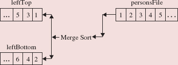
FIGURE 11.21 The first merge pass in file sorting. The files leftTop and leftBottom contain sorted blocks, and personsFile and rightBottom contain double-sized sorted blocks
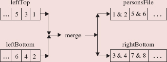
1 As always in averaging, we assume that each event is equally likely.
2 For the sake of simplicity, we assume the collection to be sorted does not contain any duplicates.
3 Technically, there is a fifth parameter. But since we assume that the entire array is being sorted, we can ignore that parameter.
4 Actually, there are fourteen versions, because for each primitive type, there is a version that allows Quick Sort to be applied to an entire array, and another version for a specified subarray.
5 The median of a collection of values is the value that would be in the middle position if the collection were sorted. For example, the median of
100 32 77 85 95
is 85. If the collection contains an even number of values, the median is the average of the two values that would be in the two middle positions if the collection were sorted. For example, the median of
100 32 77 85 95 80
is 82.5.