CHAPTER 9
Binary Trees
In this chapter we "branch" out from the linear structures of earlier chapters to introduce what is essentially a non-linear construct: the binary tree. This brief chapter focuses on the definition and properties of binary trees, and that will provide the necessary background for the next four chapters. Chapters 10 through 13 will consider various specializations of binary trees: binary search trees, AVL trees, decision trees, red-black trees, heaps, and Huffman trees. There is no question that the binary tree is one of the most important concepts in computer science. Finally, to round out the picture, Chapter 15 presents the topic of trees in general.
CHAPTER OBJECTIVES
- Understand binary-tree concepts and important properties, such as the Binary Tree Theorem and the External Path Length Theorem.
- Be able to perform various traversals of a binary tree.
9.1 Definition of Binary Tree
The following definition sets the tone for the whole chapter:
A binary tree t is either empty or consists of an element, called the root element, and two distinct binary trees, called the left subtree and right subtree of t.
We denote those subtrees as leftTree(t) and rightTree(t), respectively. Functional notation, such as leftTree(t), is utilized instead of object notation, such as t.leftTree(), because there is no binary-tree data structure. Why not? Different types of binary trees have widely differing methods—even different parameters lists—for such operations as inserting and removing. Note that the definition of a binary tree is recursive, and many of the definitions associated with binary trees are naturally recursive.
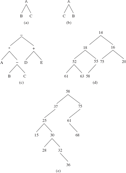
In depicting a binary tree, the root element is shown at the top, by convention. To suggest the association between the root element and the left and right subtrees, we draw a southwesterly line from the root element to the left subtree and a southeasterly line from the root element to the right subtree. Figure 9.1 shows several binary trees.
The binary tree in Figure 9.1a is different from the binary tree in Figure 9.1b because B is in the left subtree of Figure 9.1a but B is not in the left subtree of Figure 9.1b. As we will see in Chapter 15, those two binary trees are equivalent when viewed as general trees.
A subtree of a binary tree is itself a binary tree, and so Figure 9.1a has seven binary trees: the whole binary tree, the binary tree whose root element is B, the binary tree whose root element is C, and four empty binary trees. Try to calculate the total number of subtrees for the tree in Figures 9.1 c, d, and e, and hypothesize the formula to calculate the number of subtrees as a function of the number of elements.
FIGURE 9.1 Several binary trees
The next section develops several properties of binary trees, and most of the properties are relevant to the material in later chapters.
9.2 Properties of Binary Trees
In addition to "tree" and "root," botanical terms are used for several binary-tree concepts. The line from a root element to a subtree is called a branch. An element whose associated left and right subtrees are both empty is called a leaf. A leaf has no branches going down from it. In the binary tree shown in Figure 9.1e, there are four leaves: 15, 28, 36, and 68. We can determine the number of leaves in a binary tree recursively. Let t be a binary tree. The number of leaves in t, written leaves(t), can be defined as follows:
if t is empty
      leaves(t) = 0
else if t consists of a root element only
leaves(t) = 1
else
      leaves(t) = leaves(leftTree(t)) + leaves(rightTree(t))
This is a mathematical definition, not a Java method. The last line in the above definition states that the number of leaves in t is equal to the number of leaves in t 's left subtree plus the number of leaves in t 's right subtree. Just for practice, try to use this definition to calculate the number of leaves in Figure 9.1a. Of course, you can simply look at the whole tree and count the number of leaves, but the above definition of leaves(t) is atomic rather than holistic.
Each element in a binary tree is uniquely determined by its location in the tree. For example, let t be the binary tree shown in Figure 9.1c. There are two elements in t with value We can distinguish between them by referring to one of them as "the element whose value is '-' and whose location is at the root of t" and the other one as "the element whose value is '-' and whose location is at the root of the right subtree of the left subtree of t." We loosely refer to "an element" in a binary tree when, strictly speaking, we should say "the element at such and such a location."
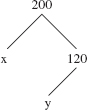
Some binary-tree concepts use familial terminology. Let t be the binary tree shown in Figure 9.2. We say that x is the parent of y and that y is the left child of x. Similarly, we say that x is the parent of z and that z is the right child of x.
In a binary tree, each element has zero, one, or two children. For example, in Figure 9.1d, 14 has two children, 18 and 16; 55 has 58 as its only child; 61 is childless, that is, it is a leaf. For any element w in a tree, we write parent(w) for the parent of w, left(w) for the left child of w and right(w) for the right child of w.
In a binary tree, the root element does not have a parent, and every other element has exactly one parent. Continuing with the terminology of a family tree, we could define sibling, grandparent, grandchild, first cousin, ancestor and descendant. For example, an element A is an ancestor of an element B if B is in the subtree whose root element is A. To put it recursively, A is an ancestor of B if A is the parent of B or if A is an ancestor of the parent of B. Try to define "descendant" recursively.
If A is an ancestor of B, the path from A to B is the sequence of elements, starting with A and ending with B, in which each element in the sequence (except the last) is the parent of the next element. For example, in Figure 9.1e, the sequence 37, 25, 30, 32 is the path from 37 to 32.
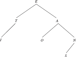
Informally, the height of a binary tree is the number of branches between the root and the farthest leaf, that is, the leaf with the most ancestors. For example, Figure 9.3 has a binary tree of height 3.
The height of the tree in Figure 9.3 (next page) is 3 because the path from E to S has three branches. Suppose for some binary tree, the left subtree has a height of 12 and the right subtree has a height of 20. What is the height of the whole tree? The answer is 21.
In general, the height of a tree is one more than the maximum of the heights of the left and right subtrees. This leads us to a recursive definition of the height of a binary tree. But first, we need to know what the base case is, namely, the height of an empty tree. We want the height of a single-element tree to be 0: there are no branches from the root element to itself. But that means that 0 is one more than the maximum heights of the left and right subtrees, which are both empty. So we need to define the height of an empty subtree to be, strangely enough, −1.
FIGURE 9.2 A binary tree with one parent and two children

FIGURE 9.3 A binary tree of height 3
Let t be a binary tree. We define height(t), the height of t, recursively as follows:
if t is empty,
height(t) = −1
else
height(t) = 1+ max (height(leftTree(t)), height(rightTree(t)))
It follows from this definition that a binary tree with a single element has height 0 because each of its empty subtrees has a height of −1. Also, the height of the binary tree in Figure 9.1a is 1. And, if you want to try some recursive gymnastics, you can verify that the height of the binary tree in Figure 9.1e is 5.
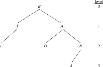
Height is a property of an entire binary tree. For each element in a binary tree, we can define a similar concept: the level of the element. Speaking non-recursively, if x is an element in a binary tree, we define level(x), the level of element x, to be the number of branches between the root element and element x. Figure 9.4 shows a binary tree, with levels.
In Figure 9.4, level(n) is 2. Notice that the level of the root element is 0, and the height of a tree is equal to the highest level in the tree. Here is a recursive definition of the level of an element. For any element x in a binary tree, we define level(x), the level of element x, as follows:
if x is the root element,
level(x) = 0
FIGURE 9.4 A binary tree, with the levels of elements shown
level(x) = 1+ level(parent(x))
An element's level is also referred to as that element's depth. Curiously, the height of a non-empty binary tree is the depth of the farthest leaf.
A two-tree is a binary tree that either is empty or in which each non-leaf has 2 branches going down from it. For example, Figure 9.5a has a two-tree and the tree in Figure 9.5b is not a two-tree.
Recursively speaking, a binary tree t is a two-tree if:
t has at most one element
or
leftTree(t) and rightTree(t) are non-empty two-trees.
A binarytreet is full if t is a two-tree with all of its leaves on the same level. For example, the tree in Figure 9.6a is full and the tree in Figure 9.6b is not full.
Recursively speaking, a binary tree t is full if:
t is empty
or
t 's left and right subtrees have the same height and both are full.
Of course, every full binary tree is a two-tree but the converse is not necessarily true. For example, the tree in Figure 9.6b is a two-tree but is not full. For full binary trees, there is a relationship between the height and number of elements in the tree. For example, the full binary tree in Figure 9.7 has a height of 2, so the tree must have exactly 7 elements:
FIGURE 9.5 (a) a two tree; (b) a binary tree that is not a two tree
FIGURE 9.6 (a) a full binary tree; (b) a binary tree that is not full
FIGURE 9.7 A full binary tree of height 2; such a tree must have exactly 7 elements
How many elements must there be in a full binary tree of height 3? Of height 4? For a full binary tree t, can you conjecture the formula for the number of elements in t as a function of height(t)? The answer can be found in Section 9.3.
A binary treet is complete if t is full through the next-to-lowest level and all of the leaves at the lowest level are as far to the left as possible. By "lowest level," we mean the level farthest from the root.
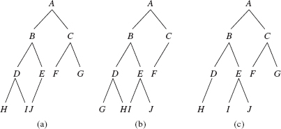
Any full binary tree is complete, but the converse is not necessarily true. For example, Figure 9.8a has a complete binary tree that is not full. The tree in Figure 9.8b is not complete because it is not full at the next-to-lowest level: C has only one child. The tree in Figure 9.8c is not complete because leaves I and J are not as far to the left as they could be.
FIGURE 9.8 Three binary trees, of which only (a) is complete
In a complete binary tree, we can associate a "position" with each element. The root element is assigned a position of 0. For any nonnegative integer i, if the element at position i has children, the position of its left child is 2i + 1 and the position of its right child is 2i + 2. For example, if a complete binary tree has ten elements, the positions of those elements are as indicated in Figure 9.9.
If we use a left shift (that is, operator <<) of one bit, we can achieve the same effect as multiplying by 2, but much faster. Then the children of the element at position i are at positions
(i << 1) + 1 and (i <<1) + 2
In Figure 9.9, the parent of the element at position 8 is in position 3, and the parent of the element in position 5 is in position 2. In general, if i is a positive integer, the position of the parent of the element in position i is in position (i — 1) >> 1; we use a right shift of one bit instead of division by 2.
The position of an element is important because we can implement a complete binary tree with a contiguous collection such as an array or an ArrayList. Specifically, we will store the element that is at position i in the tree at index i in the array. For example, Figure 9.10 shows an array with the elements from Figure 9.8a.
FIGURE 9.9 The association of consecutive integers to elements in a complete binary tree
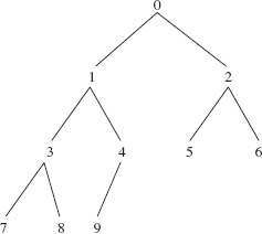
FIGURE 9.10 An array that holds the elements from the complete binary tree in Figure 9.8a
![]()
If a complete binary tree is implemented with an ArrayList object or array object, the random-access property of arrays allows us to access the children of a parent (or parent of a child) in constant time. That is exactly what we will do in Chapter 13.
We have shown how we can recursively calculate leaves(t), the number of leaves in a binary tree t, and height(t), the height of a binary tree t. We can also recursively calculate the number of elements, n (t), in t:
if t is empty
n(t) = 0
else
n(t) = 1 + n(leftTree(t)) + n(rightTree(t))
9.3 The Binary Tree Theorem
For any non-empty binary tree t, leaves(t) ≤ n(t), and leaves(t) = n(t) if and only if t consists of one element only. The phrase "if and only if" indicates that each of the individual statements follows from the other. Namely, for a non-empty binary tree t, if t consists of a single element only, then leaves(t) = n(t); and if leaves(t) = n(t), thent consists of a single element only.
The following theorem characterizes the relationships among leaves(t), height(t) and n(t).
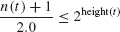
Binary Tree Theorem For any non-empty binary tree t,
- leaves(t) ≤
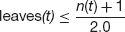
- Equality holds in part 1 if and only if t is a two-tree.
- Equality holds in part 2 if and only if t is full.
FIGURE 9.11 A binary tree t with (n(t) + 1)/2 leaves that is not a two tree
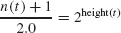
Note: Because 2.0 is the denominator of the division in part 1, the quotient is a floating point value. For example, 7/2.0 = 3.5. We cannot use integer division because of part 3: let t be the binary tree in Figure 9.11.
For the tree in Figure 9.11, leaves(t) = 2 = (n(t) + 1)/2 if we use integer division. But t is not a two-tree. Note that (n(t) + 1)/2.0 = 2.5.
Parts 3 and 4 each entail two sub-parts. For example, for part 3, we must show that if t is a non-empty two-tree, then
And if
then t must be a non-empty two-tree.
All six parts of this theorem can be proved by induction on the height of t. As it turns out, most theorems about binary trees can be proved by induction on the height of the tree. The reason for this is that if t is a binary tree, then both leftTree(t) and rightTree(t) have height less than height(t), and so the Strong Form of the Principle of Mathematical Induction (see Section A2.5 of Appendix 2) often applies. For example, Example A2.5 of Appendix 2 has a proof of part 1. The proofs of the remaining parts are left as Exercises 9.13 and 9.14, with a hint for each exercise.
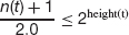
Suppose t is a full binary tree (possibly empty), then from part 4 of the Binary Tree Theorem, and the fact that any empty tree has height of —1, we have the equation
If we solve this equation for height(t), we get
height(t) = log2((n(t) + 1)/2.0)
= log2(n(t) + 1) - 1
So we can say that the height of a full tree is logarithmic in n, wheren is the number of elements in the tree; we often use n instead of n(t) when it is clear which tree we are referring to. Even if t is merely complete, its height is still logarithmic in n. See Concept Exercise 9.7. On the other hand, t could be a chain. A chain is a binary tree in which each non-leaf has exactly one child. For example, Figure 9.12 has an example of a binary tree that is a chain.
If t is a chain, then height(t) = n(t) — 1, so for chains the height is linear in n. Much of our work with trees in subsequent chapters will be concerned with maintaining logarithmic-in-n height and avoiding linear-in-n height. Basically, for inserting into or removing from certain kinds of binary trees whose height is logarithmic in n, worstTime(n) is logarithmic in n. That is why, in many applications, binary trees are preferable to lists. Recall that with both ArrayList objects and LinkedList objects, for inserting or removing at a specific index, worstTime(n) is linear in n.
FIGURE 9.12 A binary tree that is a chain: each non-leaf has exactly one child
9.4 External Path Length
You may wonder why we would be interested in adding up all the root-to-leaf path lengths, but the following definition does have some practical value. Let t be a non-empty binary tree. E(t), the external path length of t, is the sum of the depths of all the leaves in t. For example, in Figure 9.13, the sum of the depths of the leaves is 2 + 4 + 4 + 4 + 5 + 5 + 1 = 25.
The following lower bound on external path lengths yields an important result in the study of sorting algorithms (see Chapter 11).
External Path Length Theorem Let t be a binary tree with k > 0 leaves. Then
E(t) ≥ (k/2) floor (log2 k)
Proof It follows from the Binary Tree Theorem that if a nonempty binary tree is full and has height h, then the tree has 2h leaves. And we can obtain any binary tree by "pruning" a full binary tree of the same height; in so doing we reduce the number of leaves in the tree. So any non-empty binary tree of height h has no more than 2h leaves. To put that in a slightly different way, if k is any positive integer, any nonempty binary tree of height floor(log2k) has no more than k leaves. (We have to use the floor function because the height must be an integer, but log2k might not be an integer.)
FIGURE 9.13 A binary tree whose external path length is 25
Now suppose t is a nonempty binary tree whose height is floor(log2k) for some positive integer k. By the previous paragraph, t has no more than k leaves. How many of those leaves will be at level floor(log2k), the level farthest from the root? To answer that question, we ask how many leaves must be at a level less than floor(log2k). That is, how many leaves must there be in the subtree t of t formed by removing all leaves at level floor(log2k)? The height of t is floor(log2 k) — 1. Note that
floor(log2 k) - 1 = floor(log2 k - 1)
= floor(log2 k - log2 2)
= floor(log2 (k/2))
By the previous paragraph, the total number of leaves in t is no more than k/2. But every leaf in t that is at a level less than floor(log2k) is also a leaf in V. And so there must be, at least, k/2 leaves at level floor(log2k).
Each of those k/2 leaves contributes floor(log2k) to the external path length, so we must have
E(t) ≥ (k/2) floor (log2 k)
Note: This result is all we will need in Chapter 11, but at a cost of a somewhat more complicated proof, we could show that E(t) ≥ k log2 k for any non-empty two-tree with k leaves. (See Cormen, [2002] for details.)
9.5 Traversals of a Binary Tree
A traversal of a binary tree t is an algorithm that processes each element in t exactly once. In this section, we restrict our attention to algorithms only; there are no methods here. We make no attempt to declare a BinaryTree class or interface: it would not be flexible enough to support the variety of insertion and removal methods already in the Java Collections Framework. But the traversals we discuss in this section are related to code: specifically, to iterators. One of the iterators will turn up in Section 10.1.2.6, and two other iterators will appear in Chapter 15.
We identify four different kinds of traversal.
Traversal 1. in Order Traversal: Left-Root-Right The basic idea of this recursive algorithm is that we first perform an inOrder traversal of the left subtree, then we process the root element, and finally, we perform an inOrder traversal of the right subtree. Here is the algorithm—assume that t is a binary tree:
inOrder (t)
{
  if (t is not empty)
  {
      inOrder (leftTree (t));
      process the root element of t;
      inOrder (rightTree (t));
  }//if
} // inOrder traversal
Let n represent the number of elements in the tree. Corresponding to each element there are 2 subtrees, so there will be 2n recursive calls to inOrder(t). We conclude that worstTime(n) is linear in n. Ditto for averageTime(n).
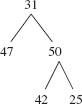
We can use this recursive description to list the elements in an inOrder traversal of the binary tree in Figure 9.14.
The tree t in Figure 9.14 is not empty, so we start by performing an inOrder traversal of leftTree(t), namely,
47
This one-element tree becomes the current version of t. Since its left subtree is empty, we process the root element of this t, namely 47. That completes the traversal of this version of t since rightTree(t) is empty. So now t again refers to the original tree. We next process t's root element, namely,
31
After that, we perform an inOrder traversal of rightTree(t), namely,

This becomes the current version of t. We start by performing an inOrder traversal of leftTree(t), namely,
42
Now this tree with one element becomes the current version of t. Since its left subtree is empty, we process t's root element, 42. The right subtree of this t is empty. So we have completed the inOrder traversal of the tree with the single element 42, and now, once again, t refers to the binary tree with 3 elements:
We next process the root element of this version of t, namely,
50
Finally, we perform an inOrder traversal of rightTree(t), namely,
25
Since the left subtree of this single-element tree t is empty, we process the root element of t, namely 25. We are now done since t 's right subtree is also empty.
FIGURE 9.15 An inOrder traversal of a binary tree
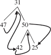
The complete listing is
47 31 42 50 25
Figure 9.15 shows the original tree, with arrows to indicate the order in which elements are processed:
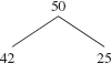
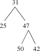
The inOrder traversal gets its name from the fact that, for a special kind of binary tree—a binary search tree—an inOrder traversal will process the elements in order. For example, Figure 9.16 has a binary search tree:
An inOrder traversal processes the elements of the tree in Figure 9.16 as follows:
25, 31, 42, 47, 50
In a binary search tree, all of the elements in the left subtree are less than the root element, which is less than all of the elements in the right subtree. What recursive property do you think will be part of the definition of a binary search tree so that an inOrder traversal processes the elements in order? Hint: the binary tree in Figure 9.17 is not a binary search tree:
We will devote Chapters 10 and 12 to the study of binary search trees.
FIGURE 9.16 A binary search tree

FIGURE 9.17 A binary tree that is not a binary search tree
Traversal 2. postOrder Traversal: Left-Right-Root The idea behind this recursive algorithm is that we perform postOrder traversals of the left and right subtrees before processing the root element. The algorithm, with t a binary tree, is:
postOrder (t)
{
   if (t is not empty)
   {
       postOrder (leftTree (t));
       postOrder (rightTree (t));
       process the root element of t;
   } //if
} // postOrder traversal
Just as with an inOrder traversal, the worstTime(n) for a postOrder traversal is linear in n because there are 2n recursive calls to postOrder(t).
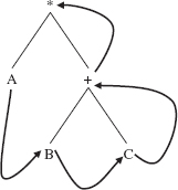
Suppose we conduct a postOrder traversal of the binary tree in Figure 9.18.
A postOrder traversal of the binary tree in Figure 9.18 will process the elements in the path shown in Figure 9.19.
In a linear form, the postOrder traversal shown in Figure 9.19 is
A B C+ *
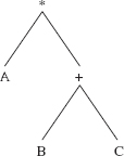
FIGURE 9.19 The path followed by a postOrder traversal of the binary tree in Figure 9.18
We can view the above binary tree as an expression tree: each non-leaf is a binary operator whose operands are the associated left and right subtrees. With this interpretation, a postOrder traversal produces postfix notation.
Traversal 3. preOrder Traversal: Root-Left-Right Here we process the root element and then perform preOrder traversals of the left and right subtrees. The algorithm, with t a binary tree, is:
preOrder (t)
{
   if (t is not empty)
   {
       process the root element of t;
       preOrder (leftTree (t));
       preOrder (rightTree (t));
   } //if
} // preOrder traversal
As with the inOrder and postOrder algorithms, worstTime(n) is linear in n.
For example, a preOrder traversal of the binary tree in Figure 9.20 will process the elements in the order indicated in Figure 9.21.
If we linearize the path in Figure 9.21, we get
* A + B C
For an expression tree, a preOrder traversal produces prefix notation.
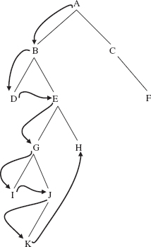
A search of a binary tree that employs a preOrder traversal is called a depth-first-search because the search goes to the left as deeply as possible before searching to the right. The search stops when (if) the element sought is found, so the traversal may not be completed. For an example of a depth-first search, Figure 9.22 shows a binary tree and the path followed by a depth-first search for H.
FIGURE 9.20 An expression tree
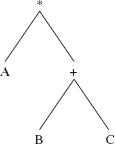
FIGURE 9.21 The path followed by a preOrder traversal of the elements in the expression tree of Figure 9.20
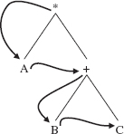
FIGURE 9.22 A depth-first search for H
The backtracking strategy from Chapter 5 includes a depth-first search, but at each stage there may be more than two choices. For example, in the maze-search, the choices are to move north, east, south, or west. Because moving north is the first option, that option will be repeatedly applied until either the goal is reached or moving north is not possible. Then a move east will be taken, if possible, and then as many moves north as possible or necessary. And so on. In Chapter 15, we will re-visit backtracking for a generalization of binary trees.
Traversal 4. breadthFirst Traversal: Level-By-Level To perform a breadth-first traversal of a non-empty binary tree t, first process the root element, then the children of the root, from left to right, then the grandchildren of the root, from left to right, and so on.
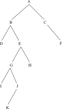
For example, suppose we perform a breadth-first traversal of the binary tree in Figure 9.23.
The order in which elements would be processed in a breadthFirst traversal of the tree in Figure 9.23
is
A B C D E F G H I J K
One way to accomplish this traversal is to generate, level-by-level, a list of (references to) non-empty subtrees. We need to retrieve these subtrees in the same order they were generated so the elements can be processed level-by-level. What kind of collection allows retrievals in the same order as insertions? A queue! Here is the algorithm, with t a binary tree:
breadthFirst (t)
{
   // queue is a queue of (references to) binary trees
   // tree is a (reference to a) binary tree
if (t  is not empty)
       {
        queue.enqueue (t);
        while (queue is not empty)
        {
            tree = queue.dequeue();
            process tree's root;
            if (leftTree (tree) is not empty)
               queue.enqueue (leftTree (tree));
            if (rightTree (tree) is not empty)
               queue.enqueue (rightTree (tree));
        } // while
       } // if t not empty
} // breadthFirst traversal
During each loop iteration, one element is processed, so worstTime(n) is linear in n.
We used a queue for a breadth-first traversal because we wanted the subtrees retrieved in the same order they were saved (First-In, First-Out). With inOrder, postOrder, and preOrder traversals, the subtrees are retrieved in the reverse of the order they were saved in (Last-In, First-Out). For each of those three traversals, we utilized recursion, which, as we saw in Chapter 8, can be replaced with an iterative, stack-based algorithm.
We will encounter this type of traversal again in Chapter 15 when we study breadth-first traversals of structures less restrictive than binary trees. Incidentally, if we are willing to be more restrictive, specifically, if we require a complete binary tree, then the tree can be implemented with an array, and a breadth-first traversal is simply an iteration through the array. The root element is at index 0, the root s left child at index 1, the root s right child at index 2, the root s leftmost grandchild at index 3, and so on.
SUMMARY
A binary tree t is either empty or consists of an element, called the root element, and two distinct binary trees, called the left subtree and right subtree of t. This is a recursive definition, and there are recursive definitions for many of the related terms: height, number of leaves, number of elements, two-tree, full tree, and so on. The inter-relationships among some of these terms is given by the
Binary Tree Theorem: For any non-empty binary tree t,
Equality holds for the first relation if and only if t is a two-tree.
Equality holds for the second relation if and only if t is a full tree.
For a binary tree t, the external path length of t, written E(t), is the sum of the distances from the root to the leaves of t. A lower bound for comparison-based sorting algorithms can be obtained from the
External Path Length Theorem: Let t be a binary tree with k ≥ 0 leaves. Then
E(t) ≥ (k/2) floor (log2 k)
There are four commonly-used traversals of a binary tree: inOrder (recursively: left subtree, root element, right subtree), postOrder (recursively: left subtree, right subtree, root element), preorder (recursively: root element, left subtree, right subtree) and breadth-first (that is, starting at the root, level-by-level, and left-to-right at each level).
CROSSWORD PUZZLE
| ACROSS | DOWN |
| 4. In a binary tree, an element with no children. | 1. A synonym of "level," the function that calculates the length of the path from the root to a given element. |
| 7. The ______ path length of a binary tree is the sum of the depths of all the leaves in the tree. | 2. Another name for "preOrder" traversal. |
| 8. A binary tree t is a _______ if t has at most one element or leftTree(t) and rightTree(t) are non-empty two-trees. | 3. A _____ is a binary tree in which each non-leaf has exactly one child. |
| 9. The only traversal in this chapter described non-recursively. | 5. A binary tree t is if t is a two-tree with all of its leaves on the same level. |
| 10. A binary tree is _______ if t is full through the next-to-lowest level and all of the leaves at the lowest level ara as far to the left as possible. | 6. An algorithm that processes each element in a binary tree exactly once. |
CONCEPT EXERCISES
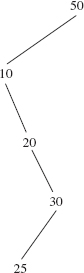
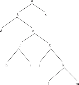
9.1 Answer the questions below about the following binary tree:
- What is the root element?
- How many elements are in the tree?
- How many leaves are in the tree?
- What is the height of the tree?
- What is the height of the left subtree?
- What is the height of the right subtree?
- What is the level of F?
- What is the depth of C?
- How many children does C have?
- What is the parent of F?
- What are the descendants of B?
- What are the ancestors of F?
- What would the output be if the elements were written out during an inOrder traversal?
- What would the output be if the elements were written out during a postOrder traversal?
- What would the output be if the elements were written out during a preOrder traversal?
- What would the output be if the elements were written out during a breadth-first traversal?
9.2
- Construct a binary tree of height 3 that has 8 elements.
- Can you construct a binary tree of height 2 that has 8 elements?
- For n going from 1 to 20, determine the minimum height possible for a binary tree with n elements.
- Based on your calculations in part c, try to develop a formula for the minimum height possible for a binary tree with n elements, where n can be any positive integer.
- Use the Principle of Mathematical Induction (Strong Form) to prove the correctness of your formula in part d.
9.3
- What is the maximum number of leaves possible in a binary tree with 10 elements? Construct such a tree.
- What is the minimum number of leaves possible in a binary tree with 10 elements? Construct such a tree.
9.4
- Construct a two-tree that is not complete.
- Construct a complete tree that is not a two-tree.
- Construct a complete two-tree that is not full.
- How many leaves are there in a two-tree with 17 elements?
- How many leaves are there in a two-tree with 731 elements?
- A non-empty two-tree must always have an odd number of elements. Why?
Hint: Use the Binary Tree Theorem and the fact that the number of leaves must be an integer.
- How many elements are there in a full binary tree of height 4?
- How many elements are there in a full binary tree of height 12?
- Use induction (original form) on the height of the tree to show that any full binary tree is a two tree.
- Use the results from part i and the Binary Tree Theorem to determine the number of leaves in a full binary tree with 63 elements.
- Construct a complete two-tree that is not full, but in which the heights of the left and right subtrees are equal.
9.5 For the following binary tree, show the order in which elements would be visited for an inOrder, postOrder, preOrder, and breadthFirst traversal.
9.6 Show that a binary tree with n elements has 2n + 1 subtrees (including the entire tree). How many of these subtrees are empty?
9.7 Show that if t is a complete binary tree, then
height(t) = floor(log2 (n (t)))
Hint: Let t be a complete binary tree of height k ≥ 0, and let t1beafullbinarytreeofheightk — 1. Then n(t 1) + 1 ≤ n(t). Use Part 4 of the Binary Tree Theorem to show that floor(log2(n(t 1) + 1)) = k, and use Part 1 of the Binary Tree Theorem to show that floor(log2(n(t))) < k + 1.
9.8 The Binary Tree Theorem is stated for non-empty binary trees. Show that parts 1, 2, and 4 hold even for an empty binary tree.
9.9 Give an example of a non-empty binary tree that is not a two-tree but
leaves(t ) = (n n(t) +1)/2
Hint: The denominator is 2, not 2.0, so integer division is performed.
9.10 Let t be a non-empty tree. Show that if
then either both subtrees of t are empty or both subtrees of t are non-empty.
Note: Do not use Part 3 of the Binary Tree Theorem. This exercise can be used in the proof of Part 3.
9.11 Show that in any complete binary tree t, at least half of the elements are leaves.
Hint: if t is empty, there are no elements, so the claim is vacuously true. If the leaf at the highest index is a right child, then t is a two-tree, and the claim follows from part 3 of the Binary Tree Theorem. Otherwise, t was formed by adding a left child to the complete two-tree with n(t) — 1elements.
9.12 Compare the inOrder traversal algorithm in Section 9.5 with the move method from the Towers of Hanoi application in Section 5.4 of Chapter 5. They have the same structure, but worstTime(n) is linear in n for the inOrder algorithm and exponential in n for the move method. Explain.
9.13 Let t be a nonempty binary tree. Use the Strong Form of the Principle of Mathematical Induction to prove each of the following parts of the Binary Tree Theorem:
- If t is a two-tree, then leaves(t) =

- If t is a full tree, then
Hint: The outline of the proof is the same as in Example A2.5 of Appendix 2.
9.14 Let t be a nonempty binary tree. Use the Strong Form of the Principle of Mathematical Induction to prove each of the following parts of the Binary Tree Theorem:
- If leaves(t) =
 then t is a two-tree.
 - If
 then t is a full tree.
Hint: The proof for both parts has the same outline. For example, here is the outline for part a:
For h = 0, 1, 2, …, let Sh be the statement
If t is a binary tree of height h and leaves(t) = ![]()
then t is a two-tree.
In the inductive case, let h be any nonnegative integer and assume that S0, S1, …, Sh are all true. To show that Sh+1 is true, let t be a binary tree of height h + 1 such that
First, show that
For any non-negative integers a, b, c, and d, if
a + b = c + dand a ≤ cand b ≥ d, then a = c and b = d.
Then, using Exercise 8.10, show that leftTree(t) and rightTree(t) are two-trees. Then, using Exercise 8.8, show that both leftTree(t) and rightTree(t) are nonempty. Conclude, from the definition of a two-tree, that t must be a two-tree.
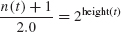
9.15 For any positive integer n, we can construct a binary tree of n elements as follows:
at level 0, there will be 1 element (the root);
at level 1, there will be 2 elements;
at level 2, there will be 3 elements;
at level 3, there will be 4 elements;
at level 4, there will be 5 elements;
...
At the level farthest from the root, there will be just enough elements so the entire tree will have n elements.
For example, if n = 12, we can construct the following tree:
Provide a Θ estimate of the height as a function of n.
Hint: Since Θ is just an estimate, we can ignore the elements at the lowest level. We seek an integer h such that
1 + 2 + 3 + 4 + … + (h + 1) = n
See Example A2.1 in Appendix 2.
Note: This exercise is contrived but, in fact, the Θ estimate of the average height of a binary tree is the same as the answer to this exercise (see Flajolet, [1981]).