Training an autoencoder is a simple process. It is an NN, where an output is the same as its input. There is an input layer, which is followed by a few hidden layers, and then after a certain depth, the hidden layers follow the reverse architecture until we reach a point where the final layer is the same as the input layer. We pass data into the network whose embedding we wish to learn.

In this example, we use images from the MNIST dataset as input. We begin our implementation by importing all the main libraries:

import tensorflow as tf
import numpy as np
import matplotlib.pyplot as plt

Then we prepare the MNIST dataset. We use the built-in input_data class from TensorFlow to load and set up the data. This class ensures that the data is downloaded and preprocessed to be consumed by the autoencoder. Therefore, basically, we don't need to do any feature engineering at all:

from tensorflow.examples.tutorials.mnist import input_data
mnist = input_data.read_data_sets("MNIST_data/",one_hot=True)

In the preceding code block, the one_hot=True parameter ensures that all the features are one hot encoded. One hot encoding is a technique by which categorical variables are converted into a form that could be fed into ML algorithms.

Next, we configure the network parameters:

learning_rate = 0.01
training_epochs = 20
batch_size = 256
display_step = 1
examples_to_show = 20

The size of input images is as follows:

n_input = 784

The sizes of the hidden features are as follows:

n_hidden_1 = 256
n_hidden_2 = 128

The final size corresponds to 28 × 28 = 784 pixels.

We need to define a placeholder variable for the input images. The data type for this tensor is set to float since the mnist values are in scale of [0, 1], and the shape is set to [None, n_input]. Defining the None parameter means that the tensor may hold an arbitrary number of images:

X = tf.placeholder("float", [None, n_input])

Then we can define the weights and biases of the network. The weights data structure contains the definition of the weights for the encoder and decoder. Notice that weights are chosen using tf.random_normal, which returns random values with a normal distribution:

weights = {
    'encoder_h1': tf.Variable
    (tf.random_normal([n_input, n_hidden_1])),
    'encoder_h2': tf.Variable
    (tf.random_normal([n_hidden_1, n_hidden_2])),
    'decoder_h1': tf.Variable
    (tf.random_normal([n_hidden_2, n_hidden_1])),
    'decoder_h2': tf.Variable
    (tf.random_normal([n_hidden_1, n_input])),
}

Similarly, we define the network's bias:

biases = {
    'encoder_b1': tf.Variable
    (tf.random_normal([n_hidden_1])),
    'encoder_b2': tf.Variable
    (tf.random_normal([n_hidden_2])),
    'decoder_b1': tf.Variable
    (tf.random_normal([n_hidden_1])),
    'decoder_b2': tf.Variable
    (tf.random_normal([n_input])),
}

We split the network modeling into two complementary fully connected networks: an encoder and a decoder. The encoder encodes the data; it takes as input an image, X, from the MNIST dataset, and performs the data encoding:

encoder_in = tf.nn.sigmoid(tf.add
                           (tf.matmul(X, 
                                      weights['encoder_h1']),
                            biases['encoder_b1']))

The input data encoding is simply a matrix multiplication operation. The input data, X, of dimension 784 is reduced to a lower dimension, 256, using matrix multiplication:

Here, W is the weight tensor, encoder_h1, and b is the bias tensor, encoder_b1. Through this operation, we have coded the initial image into a useful input for the autoencoder. The second step of the encoding procedure consists of data compression. The data represented by the input encoder_in tensor is reduced to a smaller size by means of a second matrix multiplication operation:

encoder_out = tf.nn.sigmoid(tf.add
                            (tf.matmul(encoder_in,
                                       weights['encoder_h2']),
                            biases['encoder_b2']))

The input data, encoder_in, of dimension 256 is then compressed to a lower tensor of size 128:

Here, W stands for the weight tensor, encoder_h2, while b stands for the bias tensor, encoder_b2. Notice that we used a sigmoid for the activation function for the encoder phase.

The decoder performs the inverse operation of the encoder. It decompresses the input to obtain an output of the same size of the network input. The first step of the procedure is to transform the encoder_out tensor of size 128 into a tensor of the intermediate representation of size 256:

decoder_in = tf.nn.sigmoid(tf.add
                           (tf.matmul(encoder_out,
                                      weights['decoder_h1']),
                            biases['decoder_b1']))

In formulas, it means this:

Here, W is the weight tensor, decoder_h1, of size 256 × 128, and b is the bias tensor, decoder_b1, of size 256. The final decoding operation is to decompress the data from its intermediate representation (of size 256) to a final representation (of dimension 784), which is the size of the original data:

decoder_out = tf.nn.sigmoid(tf.add
                            (tf.matmul(decoder_in,
                                       weights['decoder_h2']),
                             biases['decoder_b2']))

The y_pred parameter is set equal to decoder_out:

y_pred = decoder_out

The network will learn whether the input data, X, is equal to the decoded data, so we define the following:

y_true = X

The point of the autoencoder is to create a reduction matrix that is good at reconstructing the original data. Thus, we want to minimize the cost function. Then we define the cost function as the mean squared error between y_true and y_pred:

cost = tf.reduce_mean(tf.pow(y_true - y_pred, 2))

To optimize the cost function, we use the following RMSPropOptimizer class:

optimizer = tf.train.RMSPropOptimizer(learning_rate).minimize(cost)

Then we prepare to launch the session:

init = tf.global_variables_initializer()
with tf.Session() as sess:
    sess.run(init)

We need to set the size of the batch images to train the network:

    total_batch = int(mnist.train.num_examples/batch_size)

Start with the training cycle (the number of training_epochs is set to 10):

    for epoch in range(training_epochs):

While looping over all batches:

        for i in range(total_batch):
            batch_xs, batch_ys =
                      mnist.train.next_batch(batch_size)

Then we run the optimization procedure, feeding the execution graph with the batch set, batch_xs:

            _, c = sess.run([optimizer, cost],
                            feed_dict={X: batch_xs})

Next, we display the results for each epoch step:

        if epoch % display_step == 0:
            print(„Epoch:", ‚%04d' % (epoch+1),
                  „cost=", „{:.9f}".format(c))
    print("Optimization Finished!")

Finally, we test the model, applying the encode or decode procedure. We feed the model a subset of images, where the value of example_to_show is set to 4:

    encode_decode = sess.run(
        y_pred, feed_dict=
        {X: mnist.test.images[:examples_to_show]})

We compare the original images with their reconstructions using Matplotlib:

    f, a = plt.subplots(2, 10, figsize=(10, 2))
    for i in range(examples_to_show):
        a[0][i].imshow(np.reshape(mnist.test.images[i], (28, 28)))
        a[1][i].imshow(np.reshape(encode_decode[i], (28, 28)))
    f.show()
    plt.draw()
    plt.show()

When we run the session, we should have an output like this:

Extracting MNIST_data/train-images-idx3-ubyte.gz
Extracting MNIST_data/train-labels-idx1-ubyte.gz
Extracting MNIST_data/t10k-images-idx3-ubyte.gz
Extracting MNIST_data/t10k-labels-idx1-ubyte.gz
Epoch: 0001 cost= 0.208461761
Epoch: 0002 cost= 0.172908291
Epoch: 0003 cost= 0.153524384
Epoch: 0004 cost= 0.144243762
Epoch: 0005 cost= 0.137013704
Epoch: 0006 cost= 0.127291277
Epoch: 0007 cost= 0.125370100
Epoch: 0008 cost= 0.121299766
Epoch: 0009 cost= 0.111687921
Epoch: 0010 cost= 0.108801551
Epoch: 0011 cost= 0.105516203
Epoch: 0012 cost= 0.104304880
Epoch: 0013 cost= 0.103362709
Epoch: 0014 cost= 0.101118311
Epoch: 0015 cost= 0.098779991
Epoch: 0016 cost= 0.095374011
Epoch: 0017 cost= 0.095469855
Epoch: 0018 cost= 0.094381645
Epoch: 0019 cost= 0.090281256
Epoch: 0020 cost= 0.092290156
Optimization Finished!

Then we display the results. The first row is the original images, and the second row is the decoded images:

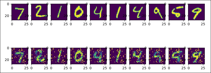
Figure 4: Original and the decoded MNIST images

As you can see, the number two differs from the original one (it still seems to be digit two like the number three). We can increase the number of epochs or change the network parameters to improve the result.