Thanks to the recent achievements of Google DeepMind in 2013 and 2016, which succeeded at reaching so-called superhuman levels in Atari games and beat the world champion Go, RL has become very interesting in of the machine learning community. This renewed interest is also due to the advent of Deep Neural Networks (DNNs) as approximation functions, bringing the potential value of this type of algorithm to an even higher level. The algorithm that has gained the most interest in recent times is definitely Deep Q-Learning. The following section introduces the Deep Q-Learning algorithm and also discusses some optimization techniques to maximize its performance.
The Q-learning base algorithm can cause tremendous problems when the number of states and possible actions increases and becomes unmanageable from a matrix point of view. Just think of the input configuration in the case of the structure used by Google to achieve the level of performance in the Atari games. State space is discrete, but the number of states is huge. This is the point where deep learning steps in. Neural networks are exceptionally good at coming up with good features for highly structured data. In fact, we can identify the Q function with a neural network, which takes the state and action as input and outputs the corresponding Q value:
Q (state; action) = value
The most common implementation of a deep neural network is pictured below:
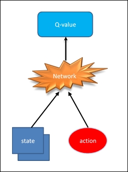
Figure 4: Common implementation of a Deep Q neural network
Alternatively, it can take the state as input and produce the corresponding value for each possible action:
Q (state) = value for each possible action
This optimized implementation can be seen in the following diagram:
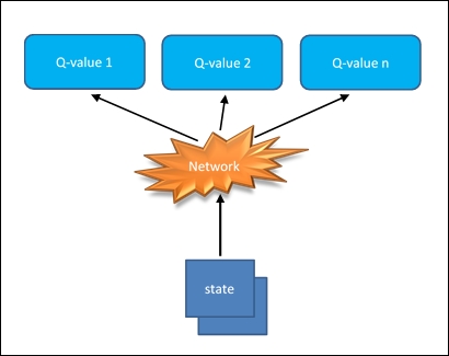
Figure 5: Optimized implementation of a Deep Q neural network
This last approach is computationally advantageous, because to update the Q value (or choose the highest Q value) we just have to take a step forward through the network and immediately we will have all Q values for all available actions.
We'll build a deep neural network that can learn to play games through RL. More specifically, we'll use Deep Q-learning to train an agent to play the Cart-Pole game.
In this game, a freely swinging pole is attached to a cart. The cart can move to the left and right, and the goal is to keep the pole upright as long as possible:

Figure 6: Cart-Pole
We simulate this game using OpenAI Gym. We need to import the required libraries:
import gym
import tensorflow as tf
import numpy as np
import time
Let's create the Cart-Pole game environment:
env = gym.make('CartPole-v0')Initialize the environment, the rewards list, and the starting time:
env.reset()
rewards = []
tic = time.time()
The env.render() statement is used here to show the window with the running simulation:
for _ in range(1000):
    env.render()
env.action_space.sample() is passed to the env.step() statement to build the next step in the simulation:
    state, reward, done, info =
           env.step
           (env.action_space.sample())
In the Cart-Pole game, there are two possible actions: moving the cart left or right. So, there are two actions we can take, encoded as 0 and 1.
Here, we take a random action:
    rewards.append(reward)
    if done:
        rewards = []
        env.reset()
toc = time.time()
After 10 seconds, the simulation ends:
if toc-tic > 10:
    env.close()
To shut the window showing the simulation, use env.close().
When we run the simulation, we have a list of rewards, as follows:
[1.0, 1.0, 1.0, 1.0, 1.0, 1.0, 1.0, 1.0, 1.0, 1.0, 1.0, 1.0, 1.0, 1.0, 1.0, 1.0, 1.0, 1.0, 1.0]
The game resets after the pole has fallen past a certain angle. The simulation returns a reward of 1.0 for each frame that it is running. The longer the game runs, the more rewards we get. So, our network's goal is to maximize the reward by keeping the pole vertical. It will do this by moving the cart to the left and the right.
We train our Q-learning agent again using the Bellman equation:
Here, s is a state, a is an action, and s' is the next state from state s and action a.
Earlier, we used this equation to learn values for a Q-table. However, there are a huge number of states available for this game. The state has four values: the position and velocity of the cart, and the position and velocity of the pole. These are all real-valued numbers, so if we ignore floating point precisions, we practically have infinite states. Instead of using a table, then, we'll replace it with a neural network that will approximate the Q-table lookup function.
The Q value is calculated by passing in a state to the network, while the output will be Q-values for each available action, with fully connected hidden layers:
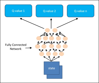
Figure 7: Deep Q-Learning
In this Cart-Pole game, we have four inputs, one for each value in the state; and two outputs, one for each action. The network weights update will take place by choosing an action and simulating the game with the chosen action. This will take us to the next state and then to the reward.
Here is a brief code snippet of the neural network used to solve the Cart-Pole problem:
import tensorflow as tf
class DQNetwork:
    def __init__(self,
                 learning_rate=0.01,
                 state_size=4,
                 action_size=2,
                 hidden_size=10,
                 name='DQNetwork'):
The hidden layers consist of two fully connected layers with ReLU activations:
            self.fc1 =tf.contrib.layers.fully_connected
                       (self.inputs_,
                        hidden_size)
            self.fc2 = tf.contrib.layers.fully_connected
                       (self.fc1,
                        hidden_size)
The output layer is a linear output layer:
            self.output = tf.contrib.layers.fully_connected
                          (self.fc2,
                           action_size,activation_fn=None)
The approximation function can suffer greatly from the presence of non-independent and identically distributed and non-stationary data (correlations between states).
This kind of problem can be overcome by using the Experience Replay method.
During the interaction between the agent and the environment, all experiences (state, action, reward, and next_state) are saved in a replay memory, which is fixed size memory and operates in First In First Out (FIFO).
Here is the implementation of the replay memory class:
from collections import deque
import numpy as np

class replayMemory():
    def __init__(self, max_size = 1000):
        self.buffer =
                    deque(maxlen=max_size)

    def build(self, experience):
        self.buffer.append(experience)

    def sample(self, batch_size):
        idx = np.random.choice
              (np.arange(len(self.buffer)),
                               size=batch_size,
                               replace=False)
        return [self.buffer[ii] for ii in idx]
This will allow the use of mini-batches of experiences taken randomly within the replay memory during the training of the network, instead of using recent experiences one after the other.
Using the experience replay method helps to mitigate the problem of sequential training data that could lead to the algorithm remaining stuck in a local minimum, denying it the chance to reach the optimal solution.
Whenever the agent has to choose which action to take, it basically has two ways that it can carry out its strategy. The first mode is called exploitation and consists of taking the best possible decision given the information obtained so far, that is, the past and stored experiences. This information is always available as a value function, which expresses which of the actions offers the greatest final cumulative return for each state-action pair.
The second mode is called exploration, and it is a strategy of making decisions that are different from what is currently considered optimal.
The exploration phase is very important, because it is used to gather information on unexplored states. In fact, it is possible that an agent that only performs the optimal action is limited to always follow the same sequence of actions without ever having had the opportunity to explore and find out that there could be strategies that, in the long run, could lead to much better results, even if this if it means the immediate gain is lower.
The policy most often used to reach the right compromise between exploration and exploitation is the greedy policy. It represents a methodology of selection of actions based on the possibility of choosing a random action with uniform probability distribution.
Let's see how to build a deep Q-Learning algorithm to solve the Cart-Pole problem.
The project is rather complex. For this reason. it has been subdivided into several file modules:
DQNetwork.py: Implements the Deep Neural Networkmemory.py: Implements the experience replay methodstart_simulation.py: Creates the Cart-Pole environment that we want to resolvesolve_cart_pole.py: Solves the Cart-Pole environment with the trained neural networkplot_result_DQN.py: Plots the final rewards versus the episodesdeepQlearning.py: The main program
The following commands provide a brief description of the implementation of the deepQlearning.py file:
import tensorflow as tf
import gym
import numpy as np
import time
import os
from create_cart_pole_env import *
from DQNetwork import *
from memory import *
from solve_cart_pole import *
from plot_result_DQN import *
The next thing to do is to define the hyperparameters used for this implementation, so we need to define the maximum number of episodes to learn from, the maximum number of steps in an episode, and the future reward discount:
train_episodes = 1000
max_steps = 200
gamma = 0.99
Exploration parameters are the exploration probability at the start, the minimum exploration probability, and the exponential decay rate for the exploration probability:
explore_start = 1.0
explore_stop = 0.01
decay_rate = 0.0001
Network parameters are the number of units in each hidden Q-network layer and the Q-network learning rate:
hidden_size = 64
learning_rate = 0.0001
Define the following memory parameters:
memory_size = 10000
batch_size = 20
Then we have the number of experiences to use to pretrain the memory:
pretrain_length = batch_size
Now we can create the environment and start the Cart-Pole simulation:
env = gym.make('CartPole-v0')
start_simulation(env)
Next, we instantiate the DNN with the hidden_size and learning_rate hyperparameters:
tf.reset_default_graph()
deepQN = DQNetwork(name='main', hidden_size=64,
                  learning_rate=0.0001)
Finally, we re-initialize the simulation:
env.reset()
Let's take a random step, from which we can get the state and the reward:
state, rew, done, _ = env.step(env.action_space.sample())
Instantiate the replayMemory object to implement the Experience Replay method:
memory = replayMemory(max_size=10000)
Take a chunk of random actions to store the relative experiences, the state and actions, using the memory.build method:
pretrain_length= 20

for j in range(pretrain_length):
    action = env.action_space.sample()
    next_state, rew, done, _ =
                env.step(env.action_space.sample())
    if done:
        env.reset()
        memory.build((state,
                      action,
                      rew,
                      np.zeros(state.shape)))
        state, rew, done, _ =
               env.step(env.action_space.sample())
    else:
        memory.build((state, action, rew, next_state))
        state = next_state
With the new experiences obtained, we can carry out the training of the neural network:
rew_list = []
train_episodes = 100
max_steps=200


with tf.Session() as sess:
    sess.run(tf.global_variables_initializer())
    step = 0
    for ep in range(1, train_episodes):
        tot_rew = 0
        t = 0
        while t < max_steps:
            step += 1
            explore_p = stop_exp + (start_exp - stop_exp)*
                        np.exp(-decay_rate*step)

            if explore_p > np.random.rand():
                action = env.action_space.sample()

else: Qs = sess.run(deepQN.output,
feed_dict={deepQN.inputs_:
state.reshape
((1, *state.shape))}) action = np.argmax(Qs)
next_state, rew, done, _ = env.step(action)
tot_rew += rew
if done:
next_state = np.zeros(state.shape)
t = max_steps
print('Episode: {}'.format(ep),
'Total rew: {}'.format(tot_rew),
'Training loss: {:.4f}'.format(loss),
'Explore P: {:.4f}'.format(explore_p))
rew_list.append((ep, tot_rew))
memory.build((state, action, rew, next_state))
env.reset()
state, rew, done, _ = env.step
(env.action_space.sample())
else:
memory.build((state, action, rew, next_state))
state = next_state
t += 1
batch_size = pretrain_length
states = np.array([item[0] for item
in memory.sample(batch_size)])
actions = np.array([item[1] for item
in memory.sample(batch_size)])
rews = np.array([item[2] for item in
memory.sample(batch_size)])
next_states = np.array([item[3] for item
in memory.sample(batch_size)])Finally, we start training the agent. The training is slow because it's rendering the frames slower than the network can train:
 target_Qs = sess.run(deepQN.output,
                                 feed_dict=
                                 {deepQN.inputs_: next_states})

            target_Qs[(next_states ==
                       np.zeros(states[0].shape))
                      .all(axis=1)] = (0, 0)

            targets = rews + 0.99 * np.max(target_Qs, axis=1)

            loss, _ = sess.run([deepQN.loss, deepQN.opt],
                                feed_dict={deepQN.inputs_: states,
                                           deepQN.targetQs_: targets,
                                           deepQN.actions_: actions})


 env = gym.make('CartPole-v0')
To test the model, we call the following function:
 solve_cart_pole(env,deepQN,state,sess)

 plot_result(rew_list)
This is the implementation of the solve_cart_pole function.py, which is used here to test the neural network on the cart pole problem:
import numpy as np

def solve_cart_pole(env,dQN,state,sess):
    test_episodes = 10
    test_max_steps = 400
    env.reset()
    for ep in range(1, test_episodes):
        t = 0
        while t < test_max_steps:
            env.render()
            Qs = sess.run(dQN.output,
                          feed_dict={dQN.inputs_: state.reshape
                                     ((1, *state.shape))})
            action = np.argmax(Qs)
            next_state, reward, done, _ = env.step(action)

            if done:
                t = test_max_steps
                env.reset()
                state, reward, done, _ =

                               env.step(env.action_space.sample())

            else:
                state = next_state
                t += 1
Finally, if we run the deepQlearning.py script we should obtain a result like this:
[2017-12-03 10:20:43,915] Making new env: CartPole-v0
[]
Episode: 1 Total reward: 7.0 Training loss: 1.1949 Explore P: 0.9993
Episode: 2 Total reward: 21.0 Training loss: 1.1786 Explore P: 0.9972
Episode: 3 Total reward: 38.0 Training loss: 1.1868 Explore P: 0.9935
Episode: 4 Total reward: 8.0 Training loss: 1.3752 Explore P: 0.9927
Episode: 5 Total reward: 9.0 Training loss: 1.6286 Explore P: 0.9918
Episode: 6 Total reward: 32.0 Training loss: 1.4313 Explore P: 0.9887
Episode: 7 Total reward: 19.0 Training loss: 1.2806 Explore P: 0.9868
……
Episode: 581 Total reward: 47.0 Training loss: 0.9959 Explore P: 0.1844
Episode: 582 Total reward: 133.0 Training loss: 21.3187 Explore P: 0.1821
Episode: 583 Total reward: 54.0 Training loss: 42.5041 Explore P: 0.1812
Episode: 584 Total reward: 95.0 Training loss: 1.5211 Explore P: 0.1795
Episode: 585 Total reward: 52.0 Training loss: 1.3615 Explore P: 0.1787
Episode: 586 Total reward: 78.0 Training loss: 1.1606 Explore P: 0.1774
…….
Episode: 984 Total reward: 199.0 Training loss: 0.2630 Explore P: 0.0103
Episode: 985 Total reward: 199.0 Training loss: 0.3037 Explore P: 0.0103
Episode: 986 Total reward: 199.0 Training loss: 256.8498 Explore P: 0.0103
Episode: 987 Total reward: 199.0 Training loss: 0.2177 Explore P: 0.0103
Episode: 988 Total reward: 199.0 Training loss: 0.3051 Explore P: 0.0103
Episode: 989 Total reward: 199.0 Training loss: 218.1568 Explore P: 0.0103
Episode: 990 Total reward: 199.0 Training loss: 0.1679 Explore P: 0.0103
Episode: 991 Total reward: 199.0 Training loss: 0.2048 Explore P: 0.0103
Episode: 992 Total reward: 199.0 Training loss: 0.4215 Explore P: 0.0102
Episode: 993 Total reward: 199.0 Training loss: 0.2133 Explore P: 0.0102
Episode: 994 Total reward: 199.0 Training loss: 0.1836 Explore P: 0.0102
Episode: 995 Total reward: 199.0 Training loss: 0.1656 Explore P: 0.0102
Episode: 996 Total reward: 199.0 Training loss: 0.2620 Explore P: 0.0102
Episode: 997 Total reward: 199.0 Training loss: 0.2358 Explore P: 0.0102
Episode: 998 Total reward: 199.0 Training loss: 0.4601 Explore P: 0.0102
Episode: 999 Total reward: 199.0 Training loss: 0.2845 Explore P: 0.0102
[2017-12-03 10:23:43,770] Making new env: CartPole-v0
>>>
The total reward increases as the training loss decreases.
During the test, the cart pole balances perfectly:
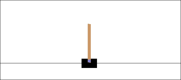
Figure 8: Resolved Cart-Pole problem
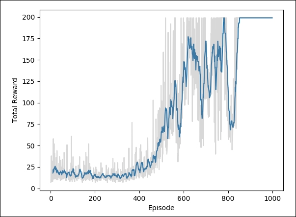
To visualize the training, we have used the plot_result() function (it is defined in the plot_result_DQN.py function).
The plot_result() function plots the total reward for each episode:
def plot_result(rew_list):
    eps, rews = np.array(rew_list).T
    smoothed_rews = running_mean(rews, 10)
    smoothed_rews = running_mean(rews, 10)
    plt.plot(eps[-len(smoothed_rews):], smoothed_rews)
    plt.plot(eps, rews, color='grey', alpha=0.3)
    plt.xlabel('Episode')
    plt.ylabel('Total Reward')
    plt.show()
The following graph shows the total reward per episode increasing as the agent improves its estimate of the value function: