
In this section, we will see how to utilize collaborative filtering to develop a recommendation engine. However, before that let's discuss the utility matrix of preferences.
In a collaborative filtering-based recommendation system, there are dimensions of entities: users and items (items refer to products, such as movies, games, and songs). As a user, you might have preferences for certain items. Therefore, these preferences must be extracted out of the data about items, users, or ratings. This data is often represented as a utility matrix, such as a user-item pair. This type of value can represent what is known about the degree of preference that the user has for a particular item.
The entry in the matrix can come from an ordered set. For example, integers 1-5 can be used to represent the number of stars that the user gave when rating items. We have already mentioned that users might not rate items very often, so most entries are unknown. Therefore, assigning 0 to unknown items would fail, which also means that the matrix is might be sparse. An unknown rating implies that we have no explicit information about the user's preference for the item.
Table 1 shows an example utility matrix. The matrix represents the rating users have given to movies on a 1-5 scale, with 5 being the highest rating. A blank entry represents the fact that the particular user has not provided any rating for that particular movie. HP1, HP2, and HP3 are acronyms for Harry Potter I, II, and III, TW stands for Twilight, and SW1, SW2, and SW3 for Star Wars episodes 1, 2, and 3. The letters A, B, C, and D represent the users:
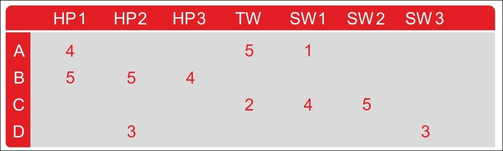
Table 1: Utility matrix (user versus movies matrix)
There are many blank entries for the user-movie pairs. This means that users have not rated those movies. In a real-life scenario, the matrix might be even sparser, with the typical user rating only a tiny fraction of all available movies. Using this matrix, the goal is to predict the blanks in the utility matrix. Now, let's see an example. Suppose we are curious to know whether user A would like SW2. It is difficult to work this out because there is not much data to work within the matrix in Table 1.
Thus, in practice, we might develop a movie recommendation engine to consider other properties of movies, such as the producer, director, leading actors, or even the similarity of their names. This way, we can compute the similarity of the movies SW1 and SW2. This similarity would drive us to conclude that since A did not like SW1, so they are unlikely to enjoy SW2 either.
However, this might not work for a larger dataset. Therefore, with much more data, we might observe that the people who rated both SW1 and SW2 were inclined to give them similar ratings. Finally, we can conclude that A would also give SW2 a low rating, similar to A's rating of SW1.
In the next section, we will see how to develop a movie recommendation engine using the collaborative filtering approach. We will see how to utilize this type of matrix.
Note
How to use the code repo: there are eight Python scripts in this code repo (that is, Deep Learning with TensorFlow_09_Codes/Collaborative Filtering/). First, execute the eda.py that performs an exploratory analysis of the dataset. Then, invoke the train.py script to perform the training. Finally, Test.py can be used for model inferencing and evaluation.
Here is the brief functionality of each script:
eda.py: This is used for the exploratory analysis of the MovieLens 1M dataset.train.py: It performs the training as well as validation. Then it prints the validation error. Finally, it creates the user-item dense table.Test.py: It restores the user vs item table generated in the training. Then evaluates all the models.run.py: It is used for model inferencing and does predictions.kmean.py: It clusters similar movies.main.py: It computes the top k movies, creates the user rating, finds top k similar items, computes the user similarity, computes the item correlation and computes the user Pearson correlation.readers.py: It reads the rating and movies data and performs some preprocessing. Finally, it prepares the dataset for the batch training.model.py: It creates the model and computes the train/validation loss.
The workflow can be described as follows:
- First, we will train a model by using the available ratings.
- Then we use the trained model to predict the missing ratings in the users versus movies matrix.
- Then, with all the predicted ratings, a new user versus movie matrix will be constructed and saved in the form of a
.pklfile. - Then, we use this matrix to make predictions of ratings for particular users.
- Finally, we will train the K-means model to cluster related movies.
Before we start implementing the movie RE, let's look at the dataset that will be used. The MovieLens 1M dataset was downloaded from the MovieLens website at http://files.grouplens.org/datasets/movielens/ml-1m.zip.
I sincerely acknowledge and thank F. Maxwell Harper and Joseph A. Konstan for making the datasets available for use. The dataset was published in MovieLens Dataset: History and Context. ACM Transactions on Interactive Intelligent Systems (TiiS) 5, 4, Article 19 (December 2015), 19 pages.
There are three files in the dataset, and they relate to movies, ratings, and users. These files contain 1,000,209 anonymous ratings of approximately 3,900 movies made by 6,040 MovieLens users who joined MovieLens in 2000.
All the ratings are contained in the ratings.dat file and are in the following format - UserID::MovieID::Rating::Timestamp:
- UserIDs range between 1 and 6,040
- MovieIDs range between 1 and 3,952
- Ratings are made on a 5-star scale
- Timestamp is represented in seconds
Note that each user has rated at least 20 movies.
Movie information is in the movies.dat file and is in the following format - MovieID::Title::Genres:
- Titles are identical to titles provided by IMDb (with the release year)
- Genres are pipe-separated (::), and each movie is categorized as action, adventure, animation, children's, comedy, crime, drama, war, documentary, fantasy, film-noir, horror, musical, mystery, romance, sci-fi, thriller, and western
User information is in the users.dat file and is in the following format - UserID::Gender::Age::Occupation::Zip-code.
All demographic information is provided voluntarily by the users and is not checked for accuracy. Only users who have provided some demographic information are included in this dataset. An M for male and F for female denotes gender.
Age is chosen from the following ranges:
- 1: Under 18
- 18: 18-24
- 25: 25-34
- 35: 35-44
- 45: 45-49
- 50: 50-55
- 56: 56+
Occupation is chosen from the following choices:
0: other, or not specified
1: academic/educator
2: artist
3: clerical/admin
4: college/grad student
5: customer service
6: doctor/health care
7: executive/managerial
8: farmer
9: homemaker
10: K-12 student
11: lawyer
12: programmer
13: retired
14: sales/marketing
15: scientist
16: self-employed
17: technician/engineer
18: tradesman/craftsman
19: unemployed
20: writer
Here, we will see an exploratory description of the dataset before we start developing the RE. I am assuming that the reader has already downloaded the MovieLens 1m dataset from http://files.grouplens.org/datasets/movielens/ml-1m.zip and unzipped it in the input directory in this code repo. Now, for this, execute the $ python3 eda.py command on the terminal:
- First, let's import the required libraries and packages:
import matplotlib.pyplot as plt
import seaborn as sns
import pandas as pd
import numpy as np
- Now let's load the users, ratings, and movies dataset and create a pandas DataFrame:
ratings_list = [i.strip().split("::") for i in open('Input/ratings.dat', 'r').readlines()] users_list = [i.strip().split("::") for i in open('Input/users.dat', 'r').readlines()] movies_list = [i.strip().split("::") for i in open('Input/movies.dat', 'r',encoding='latin-1').readlines()] ratings_df = pd.DataFrame(ratings_list, columns = ['UserID', 'MovieID', 'Rating', 'Timestamp'], dtype = int) movies_df = pd.DataFrame(movies_list, columns = ['MovieID', 'Title', 'Genres']) user_df=pd.DataFrame(users_list, columns=['UserID','Gender','Age','Occupation','ZipCode']) - The next task is to convert the categorical columns, such as
MovieID,UserID, andAge, into numerical values using the built-into_numeric()pandas function:movies_df['MovieID'] = movies_df['MovieID'].apply(pd.to_numeric) user_df['UserID'] = user_df['UserID'].apply(pd.to_numeric) user_df['Age'] = user_df['Age'].apply(pd.to_numeric)
- Let's see some examples from the user table:
print("User table description:") print(user_df.head()) print(user_df.describe()) >>> User table description: UserID Gender Age Occupation ZipCode 1 F 1 10 48067 2 M 56 16 70072 3 M 25 15 55117 4 M 45 7 02460 5 M 25 20 55455 UserID Age count 6040.000000 6040.000000 mean 3020.500000 30.639238 std 1743.742145 12.895962 min 1.000000 1.000000 25% 1510.750000 25.000000 50% 3020.500000 25.000000 75% 4530.250000 35.000000 max 6040.000000 56.000000 - Let's see some info from the rating dataset:
print("Rating table description:") print(ratings_df.head()) print(ratings_df.describe()) >>> Rating table description: UserID MovieID Rating Timestamp 1 1193 5 978300760 1 661 3 978302109 1 914 3 978301968 1 3408 4 978300275 1 2355 5 978824291 UserID MovieID Rating Timestamp count 1.000209e+06 1.000209e+06 1.000209e+06 1.000209e+06 mean 3.024512e+03 1.865540e+03 3.581564e+00 9.722437e+08 std 1.728413e+03 1.096041e+03 1.117102e+00 1.215256e+07 min 1.000000e+00 1.000000e+00 1.000000e+00 9.567039e+08 25% 1.506000e+03 1.030000e+03 3.000000e+00 9.653026e+08 50% 3.070000e+03 1.835000e+03 4.000000e+00 9.730180e+08 75% 4.476000e+03 2.770000e+03 4.000000e+00 9.752209e+08 max 6.040000e+03 3.952000e+03 5.000000e+00 1.046455e+09 - Let's look at some info from the movie dataset:
>>> print("Movies table description:") print(movies_df.head()) print(movies_df.describe()) >>> Movies table description: MovieID Title Genres 0 1 Toy Story (1995) Animation|Children's|Comedy 1 2 Jumanji (1995) Adventure|Children's|Fantasy 2 3 Grumpier Old Men (1995) Comedy|Romance 3 4 Waiting to Exhale (1995) Comedy|Drama 4 5 Father of the Bride Part II (1995) Comedy MovieID count 3883.000000 mean 1986.049446 std 1146.778349 min 1.000000 25% 982.500000 50% 2010.000000 75% 2980.500000 max 3952.000000 - Now let's see the top five most rated movies:
print("Top ten most rated movies:") print(ratings_df['MovieID'].value_counts().head()) >>> Top 10 most rated movies with title and rating count: American Beauty (1999) 3428 Star Wars: Episode IV - A New Hope (1977) 2991 Star Wars: Episode V - The Empire Strikes Back (1980) 2990 Star Wars: Episode VI - Return of the Jedi (1983) 2883 Jurassic Park (1993) 2672 Saving Private Ryan (1998) 2653 Terminator 2: Judgment Day (1991) 2649 Matrix, The (1999) 2590 Back to the Future (1985) 2583 Silence of the Lambs, The (1991) 2578 - Now let's look at the movie rating distribution. For this, let's use a histogram plot, that demonstrates an important pattern where votes are distributed normally:
plt.hist(ratings_df.groupby(['MovieID'])['Rating'].mean().sort_values(axis=0, ascending=False))
plt.title("Movie rating Distribution")
plt.ylabel('Count of movies')
plt.xlabel('Rating');
plt.show()
>>>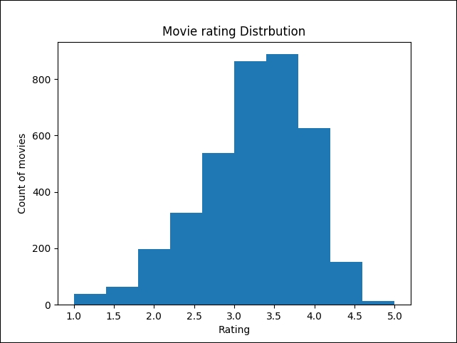
Figure 3: Movie rating distribution
- Let's see how the ratings are distributed across different age groups:
user_df.Age.plot.hist()
plt.title("Distribution of users (by ages)")
plt.ylabel('Count of users')
plt.xlabel('Age');
plt.show()
>>>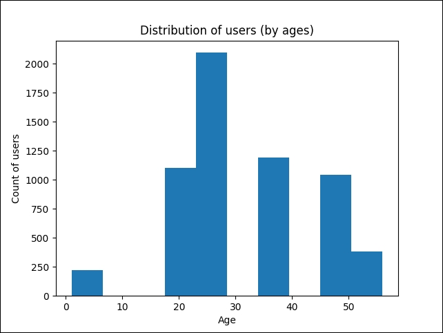
Figure 4: Distribution of users by age
- Now let's see the highest-rated movie with a minimum of 150 ratings:
movie_stats = df.groupby('Title').agg({'Rating': [np.size, np.mean]}) print("Highest rated movie with minimum 150 ratings") print(movie_stats.Rating[movie_stats.Rating['size'] > 150].sort_values(['mean'],ascending=[0]).head()) >>> Top 5 and a highest rated movie with a minimum of 150 ratings----------------------------------------------------------- Title size mean Seven Samurai (The Magnificent Seven) 628 4.560510 Shawshank Redemption, The (1994) 2227 4.554558 Godfather, The (1972) 2223 4.524966 Close Shave, A (1995) 657 4.520548 Usual Suspects, The (1995) 1783 4.517106 - Let's look at gender bias in movie ratings, that is, how the movies' ratings compare by gender of the reviewer:
>>> pivoted = df.pivot_table(index=['MovieID', 'Title'], columns=['Gender'], values='Rating', fill_value=0) print("Gender biasing towards movie rating") print(pivoted.head()) - We can now have a look at gender bias towards movie ratings and the difference between them, that is, how men and women rate the movies differently:
pivoted['diff'] = pivoted.M - pivoted.F
print(pivoted.head())
>>>
Gender                                                   F                       M                      diff
MovieID Title
1  Toy Story (1995)                            4.87817        4.130552                -0.057265
2  Jumanji (1995)                               3.278409      3.175238                -0.103171
3  Grumpier Old Men (1995)             3.073529      2.994152               -0.079377
4  Waiting to Exhale (1995)              2.976471        2.482353              -0.494118
5  Father of the Bride Part II (1995)  3.212963       2.888298               -0.324665
- From the preceding output, it is clear that in most cases, men provided higher ratings than women. Now that we have seen some info and statistics about the dataset, it is time to build our TensorFlow recommendation model.
In this example, we will see how to recommend the top k movies (where k is the number of movies), predict user ratings and recommend the top k similar items (where k is the number of items). Then we will see how to compute user similarity.
Then we will see the item-item correlation and user-user correlation using Pearson's correlation algorithm. Finally, we will see how to cluster similar movies using the K-means algorithm.
In other words, we will make a movie recommendation engine using the collaborative filtering approach and K-means to cluster similar movies.
Distance calculation: There are other ways to calculate the distance as well. For example:
- Chebyshev distance can be used to measure the distance by considering only the most notable dimensions.
- The Hamming distance algorithm can identify the difference between two strings.
- Mahalanobis distance can be used to normalize the covariance matrix.
- Manhattan distance is used to measure the distance by considering only axis-aligned directions.
- The Haversine distance is used to measure the great-circle distances between two points on a sphere from the location.
Considering these distance-measuring algorithms, it is clear that the Euclidean distance algorithm would be the most appropriate to solve our purpose of distance calculation in the K-means algorithm
In summary, here is the workflow that will be used to develop this model:
- First, train a model by using the available ratings.
- Use that trained model to predict missing ratings in users versus movies matrix.
- With all the predicted ratings, the users versus movies matrix become the trained users versus movies matrix, and we save both in the form of a
.pklfile. - Then, we use the users versus movies matrix, or trained users versus movies matrix by the trained argument, for further processing.
Before training the model, the very first job is to prepare the training set by utilizing all of the available datasets.
For this part, use the train.py script, which is dependent on other scripts. We will see the dependencies:
- First, let's import necessary packages and modules:
from collections import deque
from six import next
import readers
import os
import tensorflow as tf
import numpy as np
import model as md
import pandas as pd
import time
import matplotlib.pyplot as plt
- Then we set the random seed for reproducibility:
np.random.seed(12345)
- The next task is to define the training parameters. Let's define the required data parameters, such as the location of the ratings dataset, the batch size, the dimension of SVD, the maximum epochs, and the checkpoint directory:
data_file ="Input/ratings.dat"# Input user-movie-rating information file
batch_size = 100 #Batch Size (default: 100)
dims =15 #Dimensions of SVD (default: 15)
max_epochs = 50 # Maximum epoch (default: 25)
checkpoint_dir ="save/" #Checkpoint directory from training run
 val = True #True if Folders with files and False if single file
is_gpu = True # Want to train model with GPU
- We also need some other parameters, such as allowing soft placement and log device placement:
allow_soft_placement = True #Allow device soft device placement
log_device_placement=False #Log placement of ops on devices
- We don't want to contaminate our fresh training with old metadata, or checkpoint and model files, so let's remove them if there are any:
print("Start removing previous Files ...") if os.path.isfile("model/user_item_table.pkl"): os.remove("model/user_item_table.pkl") if os.path.isfile("model/user_item_table_train.pkl"): os.remove("model/user_item_table_train.pkl") if os.path.isfile("model/item_item_corr.pkl"): os.remove("model/item_item_corr.pkl") if os.path.isfile("model/item_item_corr_train.pkl"): os.remove("model/item_item_corr_train.pkl") if os.path.isfile("model/user_user_corr.pkl"): os.remove("model/user_user_corr.pkl") if os.path.isfile("model/user_user_corr_train.pkl"): os.remove("model/user_user_corr_train.pkl") if os.path.isfile("model/clusters.csv"): os.remove("model/clusters.csv") if os.path.isfile("model/val_error.pkl"): os.remove("model/val_error.pkl") print("Done ...") >>> Start removing previous Files... Done... - Then let's define the checkpoint directory. TensorFlow assumes this directory already exists, so we need to create it:
checkpoint_prefix = os.path.join(checkpoint_dir, "model") if not os.path.exists(checkpoint_dir): os.makedirs(checkpoint_dir) - Before getting into the data, let's set the number of samples per batch, the dimension of the data, and the number of times the network sees all the training data:
batch_size =batch_size
dims =dims
max_epochs =max_epochs
- Now let's specify the devices to be used for all TensorFlow computations, CPU or GPU:
if is_gpu: place_device = "/gpu:0" else: place_device="/cpu:0" - Now we read the rating file with the delimiter,
::, through theget_data()function. A sample column consists of user ID, item ID, rating, and timestamp, for example, 3::1196::4::978297539. Then the above code does the purely integer-location based indexing for selection by position. After that, it splits the data into training and testing, 75% for training and 25% for testing. Finally, it uses the indices to separate the data and returns the data frame to use for the training:def get_data(): print("Inside get data ...") df = readers.read_file(data_file, sep="::") rows = len(df) df = df.iloc[np.random.permutation(rows)].reset_index(drop=True) split_index = int(rows * 0.75) df_train = df[0:split_index] df_test = df[split_index:].reset_index(drop=True) print("Done !!!") print(df.shape) return df_train, df_test,df['user'].max(),df['item'].max() - We then clip the limit of the values in an array: given an interval, values outside the interval are clipped to the edges of the interval. For example, if an interval of [0, 1] is specified, values smaller than 0 become 0, and values larger than 1 become 1:
def clip(x):
    return np.clip(x, 1.0, 5.0)
We then invoke the read_data() method to read data from the ratings file to build a TensorFlow model:
df_train, df_test,u_num,i_num = get_data()
>>>
Inside get data...
Done!!!
- We then define the number of users in the dataset who rated the movies, and the number of movies in the dataset:
u_num = 6040 # Number of users in the dataset
i_num = 3952 # Number of movies in the dataset
- Now let's generate the number of samples per batch:
samples_per_batch = len(df_train) // batch_size print("Number of train samples %d, test samples %d, samples per batch %d" % (len(df_train), len(df_test), samples_per_batch)) >>> Number of train samples 750156, test samples 250053, samples per batch 7501 - Now, using a shuffle iterator, we generate random batches. In training, this helps to prevent a biased result as well as overfitting:
iter_train = readers.ShuffleIterator([df_train["user"], df_train["item"],df_train["rate"]], batch_size=batch_size)
- For more on this class, refer to the
readers.pyscript. For your convenience, here is the source of this class:class ShuffleIterator(object): def __init__(self, inputs, batch_size=10): self.inputs = inputs self.batch_size = batch_size self.num_cols = len(self.inputs) self.len = len(self.inputs[0]) self.inputs = np.transpose(np.vstack([np.array(self.inputs[i]) for i in range(self.num_cols)])) def __len__(self): return self.len def __iter__(self): return self def __next__(self): return self.next() def next(self): ids = np.random.randint(0, self.len, (self.batch_size,)) out = self.inputs[ids, :] return [out[:, i] for i in range(self.num_cols)] - Then we sequentially generate one-epoch batches for testing (see
train.py):iter_test = readers.OneEpochIterator([df_test["user"], df_test["item"], df_test["rate"]], batch_size=-1)
- For more on this class, refer to the
readers.pyscript. For your convenience, here is the source of this class:class OneEpochIterator(ShuffleIterator): def __init__(self, inputs, batch_size=10): super(OneEpochIterator, self).__init__(inputs, batch_size=batch_size) if batch_size > 0: self.idx_group = np.array_split(np.arange(self.len), np.ceil(self.len / batch_size)) else: self.idx_group = [np.arange(self.len)] self.group_id = 0 def next(self): if self.group_id >= len(self.idx_group): self.group_id = 0 raise StopIteration out = self.inputs[self.idx_group[self.group_id], :] self.group_id += 1 return [out[:, i] for i in range(self.num_cols)] - Now it's time to create the TensorFlow placeholders:
user_batch = tf.placeholder(tf.int32, shape=[None], name="id_user")
item_batch = tf.placeholder(tf.int32, shape=[None], name="id_item")
rate_batch = tf.placeholder(tf.float32, shape=[None])
- Now that our training set and the placeholders are ready to hold the batches of training values, it time to instantiate the model. For this, we use the
model()method and use l2 regularization to avoid overfitting (see themodel.pyscript):infer, regularizer = md.model(user_batch, item_batch, user_num=u_num, item_num=i_num, dim=dims, device=place_device)
The
model()method is as follows:def model(user_batch, item_batch, user_num, item_num, dim=5, device="/cpu:0"): with tf.device("/cpu:0"): # Using a global bias term bias_global = tf.get_variable("bias_global", shape=[]) # User and item bias variables: get_variable: Prefixes the name with the current variable # scope and performs reuse checks. w_bias_user = tf.get_variable("embd_bias_user", shape=[user_num]) w_bias_item = tf.get_variable("embd_bias_item", shape=[item_num]) # embedding_lookup: Looks up 'ids' in a list of embedding tensors # Bias embeddings for user and items, given a batch bias_user = tf.nn.embedding_lookup(w_bias_user, user_batch, name="bias_user") bias_item = tf.nn.embedding_lookup(w_bias_item, item_batch, name="bias_item") # User and item weight variables w_user = tf.get_variable("embd_user", shape=[user_num, dim], initializer=tf.truncated_normal_initializer(stddev=0.02)) w_item = tf.get_variable("embd_item", shape=[item_num, dim], initializer=tf.truncated_normal_initializer(stddev=0.02)) # Weight embeddings for user and items, given a batch embd_user = tf.nn.embedding_lookup(w_user, user_batch, name="embedding_user") embd_item = tf.nn.embedding_lookup(w_item, item_batch, name="embedding_item") # reduce_sum: Computes the sum of elements across dimensions of a tensor infer = tf.reduce_sum(tf.multiply(embd_user, embd_item), 1) infer = tf.add(infer, bias_global) infer = tf.add(infer, bias_user) infer = tf.add(infer, bias_item, name="svd_inference") # l2_loss: Computes half the L2 norm of a tensor without the sqrt regularizer = tf.add(tf.nn.l2_loss(embd_user), tf.nn.l2_loss(embd_item), name="svd_regularizer") return infer, regularizer - Now let's define the training ops (see more in
models.pyscript):_, train_op = md.loss(infer, regularizer, rate_batch, learning_rate=0.001, reg=0.05, device=place_device)
The loss() method is as follows:
def loss(infer, regularizer, rate_batch, learning_rate=0.1, reg=0.1, device="/cpu:0"):
    with tf.device(device):
        cost_l2 = tf.nn.l2_loss(tf.subtract(infer, rate_batch))
        penalty = tf.constant(reg, dtype=tf.float32, shape=[], name="l2")
        cost = tf.add(cost_l2, tf.multiply(regularizer, penalty))
        train_op = tf.train.FtrlOptimizer(learning_rate).minimize(cost)
return cost, train_op- Once we have instantiated the model and training ops, we can save the model for future use:
saver = tf.train.Saver()
init_op = tf.global_variables_initializer()
session_conf = tf.ConfigProto(
  allow_soft_placement=allow_soft_placement, log_device_placement=log_device_placement)
- Now we start training the model:
with tf.Session(config = session_conf) as sess: sess.run(init_op) print("%s %s %s %s" % ("Epoch", "Train err", "Validation err", "Elapsed Time")) errors = deque(maxlen=samples_per_batch) train_error=[] val_error=[] start = time.time() for i in range(max_epochs * samples_per_batch): users, items, rates = next(iter_train) _, pred_batch = sess.run([train_op, infer], feed_dict={user_batch: users, item_batch: items, rate_batch: rates}) pred_batch = clip(pred_batch) errors.append(np.power(pred_batch - rates, 2)) if i % samples_per_batch == 0: train_err = np.sqrt(np.mean(errors)) test_err2 = np.array([]) for users, items, rates in iter_test: pred_batch = sess.run(infer, feed_dict={user_batch: users, item_batch: items}) pred_batch = clip(pred_batch) test_err2 = np.append(test_err2, np.power(pred_batch - rates, 2)) end = time.time() print("%02d %.3f %.3f %.3f secs" % (i // samples_per_batch, train_err, np.sqrt(np.mean(test_err2)), end - start)) train_error.append(train_err) val_error.append(np.sqrt(np.mean(test_err2))) start = end saver.save(sess, checkpoint_prefix) pd.DataFrame({'training error':train_error,'validation error':val_error}).to_pickle("val_error.pkl") print("Training Done !!!") sess.close() - The preceding code carries out the training and saves the errors in a pickle file. Finally, it prints the training and validation error and the time taken:
>>>
Epoch    Train err    Validation err    Elapsed Time
00          2.816          2.812                0.118 secs
01          2.813          2.812                4.898 secs
…          …               …                     …
48          2.770          2.767                1.618 secs
49          2.765          2.760                1.678 secs
Training Done!!!
The result is abridged, only a few steps have been shown. Now let's see these errors graphically:
error = pd.read_pickle("val_error.pkl")
error.plot(title="Training vs validation error (per epoch)")
plt.ylabel('Error/loss')
plt.xlabel('Epoch');
plt.show()
>>>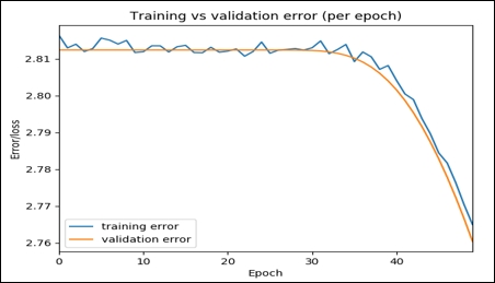
Figure 5: Training versus validation error per epoch
This graph shows that over time, both the training and the validation errors decrease, which means that we are walking in the correct direction. Nevertheless, you could still try to increase the steps and see if these two values can be further reduced, which means better accuracy.
The following code performs the model inferencing using the saved model and it prints the overall validation error:
if val:
    print("Validation ...")
    init_op = tf.global_variables_initializer()
    session_conf = tf.ConfigProto(
      allow_soft_placement=allow_soft_placement,
      log_device_placement=log_device_placement)
    with tf.Session(config = session_conf) as sess:
        new_saver = tf.train.import_meta_graph("{}.meta".format(checkpoint_prefix))
        new_saver.restore(sess, tf.train.latest_checkpoint(checkpoint_dir))
        test_err2 = np.array([])
        for users, items, rates in iter_test:
            pred_batch = sess.run(infer, feed_dict={user_batch: users, item_batch: items})
            pred_batch = clip(pred_batch)
            test_err2 = np.append(test_err2, np.power(pred_batch - rates, 2))
            print("Validation Error: ",np.sqrt(np.mean(test_err2)))
    print("Done !!!")
sess.close()
>>>
Validation Error:  2.14626890224
Done!!!The following method creates the user-item dataframe. It is used to create a trained DataFrame. All the missing values in the user-item table are filled in here using the SVD trained model. It takes the ratings dataframe and stores all the user ratings for all the movies. Finally, it generates a filled ratings dataframe, where the rows are the users and the columns are the items:
def create_df(ratings_df=readers.read_file(data_file, sep="::")):
    if os.path.isfile("model/user_item_table.pkl"):
        df=pd.read_pickle("user_item_table.pkl")
    else:
        df = ratings_df.pivot(index = 'user', columns ='item', values = 'rate').fillna(0)
        df.to_pickle("user_item_table.pkl")

    df=df.T
    users=[]
    items=[]
    start = time.time()
    print("Start creating user-item dense table")
    total_movies=list(ratings_df.item.unique())

    for index in df.columns.tolist():
        #rated_movies=ratings_df[ratings_df['user']==index].drop(['st', 'user'], axis=1)
        rated_movie=[]
        rated_movie=list(ratings_df[ratings_df['user']==index].drop(['st', 'user'], axis=1)['item'].values)
        unseen_movies=[]
        unseen_movies=list(set(total_movies) - set(rated_movie))

        for movie in unseen_movies:
            users.append(index)
            items.append(movie)
    end = time.time()

    print(("Found in %.2f seconds" % (end-start)))
    del df
    rated_list = []

    init_op = tf.global_variables_initializer()
    session_conf = tf.ConfigProto(
      allow_soft_placement=allow_soft_placement,
      log_device_placement=log_device_placement)

    with tf.Session(config = session_conf) as sess:
        #sess.run(init_op)
        print("prediction started ...")
        new_saver = tf.train.import_meta_graph("{}.meta".format(checkpoint_prefix))
        new_saver.restore(sess, tf.train.latest_checkpoint(checkpoint_dir))
        test_err2 = np.array([])
        rated_list = sess.run(infer, feed_dict={user_batch: users, item_batch: items})
        rated_list = clip(rated_list)
        print("Done !!!")
    sess.close()

    df_dict={'user':users,'item':items,'rate':rated_list}
    df = ratings_df.drop(['st'],axis=1).append(pd.DataFrame(df_dict)).pivot(index = 'user', columns ='item', values = 'rate').fillna(0)
    df.to_pickle("user_item_table_train.pkl")
    return df
Now let's invoke the preceding method to generate the user-item table as a pandas dataframe:
create_df(ratings_df = readers.read_file(data_file, sep="::"))
This line will create the user versus item table for the training set and save the dataframe as a user_item_table_train.pkl file in your specified directory.
For this section, refer to the kmean.py script. This script takes the rating data file as input and returns movies along with their respective clusters.
More technically, the aim of this section is to find similar movies; for example, user 1 liked movie 1, and because movie 1 and movie 2 are similar, the user would like movie 2. Let's get started by importing required packages and modules:
import tensorflow as tf
import numpy as np
import pandas as pd
import time
import readers
import matplotlib.pyplot as plt
import seaborn as sns
from sklearn.decomposition import PCA
Now let's define the data parameters to be used: the path of the rating data file, number of clusters, K, and maximum number of iterations. Additionally, we also define whether we would like to use a trained user versus item matrix:
data_file = "Input/ratings.dat" #Data source for the positive data
 K = 5 # Number of clusters
 MAX_ITERS =1000 # Maximum number of iterations
 TRAINED = False # Use TRAINED user vs item matrix
Then the k_mean_clustering () method is defined. It returns the movies along with their respective clusters. It takes the ratings dataset, ratings_df, which is a rating data frame. It then stores all the user ratings for respective movies, K is the number of clusters, MAX_ITERS is the maximum number of recommendations, and TRAINED is a Boolean type that signifies whether to use the trained user versus movie table or the untrained one.
Tip
How to find the optimal K value
Here we set the value of K naively. However, to fine-tune the clustering performance, we can use a heuristic approach called Elbow method. We start from K = 2, then, we run the K-means algorithm by increasing K and observe the value of the cost function (CF) using WCSS. At some point, a big drop in CF will happen. Nevertheless, the improvement then becomes marginal with an increasing value of K. In summary, we can pick the K after the last big drop of WCSS as an optimal one.
Finally, the k_mean_clustering() function returns a list of movies/items and a list of clusters:
def k_mean_clustering(ratings_df,K,MAX_ITERS,TRAINED=False):
    if TRAINED:
        df=pd.read_pickle("user_item_table_train.pkl")
    else:
        df=pd.read_pickle("user_item_table.pkl")
    df = df.T
    start = time.time()
    N=df.shape[0]

    points = tf.Variable(df.as_matrix())
    cluster_assignments = tf.Variable(tf.zeros([N], dtype=tf.int64))
    centroids = tf.Variable(tf.slice(points.initialized_value(), [0,0], [K,df.shape[1]]))
    rep_centroids = tf.reshape(tf.tile(centroids, [N, 1]), [N, K, df.shape[1]])
    rep_points = tf.reshape(tf.tile(points, [1, K]), [N, K, df.shape[1]])
    sum_squares = tf.reduce_sum(tf.square(rep_points - rep_centroids),reduction_indices=2)

    best_centroids = tf.argmin(sum_squares, 1)    did_assignments_change = tf.reduce_any(tf.not_equal(best_centroids, cluster_assignments))

    means = bucket_mean(points, best_centroids, K)

    with tf.control_dependencies([did_assignments_change]):
        do_updates = tf.group(
            centroids.assign(means),
            cluster_assignments.assign(best_centroids))

    init = tf.global_variables_initializer()
    sess = tf.Session()
    sess.run(init)
    changed = True
    iters = 0

    while changed and iters < MAX_ITERS:
        iters += 1
        [changed, _] = sess.run([did_assignments_change, do_updates])
    [centers, assignments] = sess.run([centroids, cluster_assignments])
    end = time.time()

    print (("Found in %.2f seconds" % (end-start)), iters, "iterations")
    cluster_df=pd.DataFrame({'movies':df.index.values,'clusters':assignments})

    cluster_df.to_csv("clusters.csv",index=True)
    return assignments,df.index.values
In the preceding code, we have a silly initialization in a sense that we use the first K points as the starting centroids. In the real world, it can be further improved.
In the preceding code block, we replicate N copies of each centroid and K copies of each data point. Then we subtract and compute the sum of squared distances. We then use the argmin to select the lowest-distance point. However, we do not write the assigned clusters variable until after computing whether the assignments have changed, hence with dependencies.
If you look at the preceding code carefully, there is a function called bucket_mean(). It takes the data points, the best centroids, and the number of the tentative cluster, K, and computes the mean to use in cluster computation:
def bucket_mean(data, bucket_ids, num_buckets):
    total = tf.unsorted_segment_sum(data, bucket_ids, num_buckets)
    count = tf.unsorted_segment_sum(tf.ones_like(data), bucket_ids, num_buckets)
    return total / count
Once we have trained our K-means model, the next task is to visualize those clusters representing similar movies. For this, we have a function called showClusters(), which takes the user-item table, the clustered data written in a CSV file (clusters.csv), the number of principal components (the default is 2), and the SVD solver (possible values are randomized and full).
The thing is, in a 2D space it would be difficult to plot all the data points representing the movie clusters. For this reason, we have applied Principal Component Analysis (PCA) to reduce the dimensionality without sacrificing the quality much:
    user_item=pd.read_pickle(user_item_table)
    cluster=pd.read_csv(clustered_data, index_col=False)
    user_item=user_item.T
    pcs = PCA(number_of_PCA_components, svd_solver)
    cluster['x']=pcs.fit_transform(user_item)[:,0]
    cluster['y']=pcs.fit_transform(user_item)[:,1]
    fig = plt.figure()
    ax = plt.subplot(111)
    ax.scatter(cluster[cluster['clusters']==0]['x'].values,cluster[cluster['clusters']==0]['y'].values,color="r", label='cluster 0')
    ax.scatter(cluster[cluster['clusters']==1]['x'].values,cluster[cluster['clusters']==1]['y'].values,color="g", label='cluster 1')
    ax.scatter(cluster[cluster['clusters']==2]['x'].values,cluster[cluster['clusters']==2]['y'].values,color="b", label='cluster 2')
    ax.scatter(cluster[cluster['clusters']==3]['x'].values,cluster[cluster['clusters']==3]['y'].values,color="k", label='cluster 3')
    ax.scatter(cluster[cluster['clusters']==4]['x'].values,cluster[cluster['clusters']==4]['y'].values,color="c", label='cluster 4')
    ax.legend()
    plt.title("Clusters of similar movies using K-means")
    plt.ylabel('PC2')
    plt.xlabel('PC1');
    plt.show()
Well done. We will evaluate our model and plot the clusters in the evaluation step.
For this I have written a function called prediction(). It takes the sample input about users and items (in this case, movies), and creates TensorFlow placeholders from the graph by name. It then evaluates those tensors. In the following code, it is to be noted that TensorFlow assumes that the checkpoint directory already exists, so make sure that it already exists. For details on this step refer to the run.py file. Note that this script does not show any result but a function from this script named prediction is further invoked in the main.py script for making predictions:
def prediction(users=predicted_user, items=predicted_item, allow_soft_placement=allow_soft_placement,
log_device_placement=log_device_placement, checkpoint_dir=checkpoint_dir):
    rating_prediction=[]
    checkpoint_prefix = os.path.join(checkpoint_dir, "model")
    graph = tf.Graph()
    with graph.as_default():
        session_conf = tf.ConfigProto(allow_soft_placement=allow_soft_placement,log_device_placement=log_device_placement)
        with tf.Session(config = session_conf) as sess:
            new_saver = tf.train.import_meta_graph("{}.meta".format(checkpoint_prefix))
            new_saver.restore(sess, tf.train.latest_checkpoint(checkpoint_dir))
            user_batch = graph.get_operation_by_name("id_user").outputs[0]
            item_batch = graph.get_operation_by_name("id_item").outputs[0]
            predictions = graph.get_operation_by_name("svd_inference").outputs[0]
            pred = sess.run(predictions, feed_dict={user_batch: users, item_batch: items})
            pred = clip(pred)
        sess.close()
    return  pred
We will see how we could use this method to predict the top k movies and user ratings for movies. In the preceding code segment, clip() is a user-defined function that limits the values in an array. Here is the implementation:
def clip(x):
    return np.clip(x, 1.0, 5.0) # rating 1 to 5
Now let's see how we could use the prediction() method to make a set of movie ratings predictions by a user:
def user_rating(users,movies):
    if type(users) is not list: users=np.array([users])
    if type(movies) is not list:
        movies=np.array([movies])
    return prediction(users,movies)
The preceding function returns a user rating for respective user. It takes a list of one or more numbers, a list of one or more user IDs, and a list of one or more numbers and a list of one or more movie IDs. Finally, it returns a list of predicted movies.
The following method extracts the top k movies that a user has not seen where k is an arbitrary integer such as 10. The name of the function is top_k_movies(). It returns the top k movies for a certain user. It takes a list of user IDs and the rating dataframe. It then stores all the user ratings for these movies. The output is a dictionary containing the user ID as the key and the list of the top k movies for that user as the value:
def top_k_movies(users,ratings_df,k):
    dicts={}
    if type(users) is not list:
        users = [users]
    for user in users:
        rated_movies = ratings_df[ratings_df['user']==user].drop(['st', 'user'], axis=1)
        rated_movie = list(rated_movies['item'].values)
        total_movies = list(ratings_df.item.unique())
        unseen_movies = list(set(total_movies) - set(rated_movie))
        rated_list = []
        rated_list = prediction(np.full(len(unseen_movies),user),np.array(unseen_movies))
        useen_movies_df = pd.DataFrame({'item': unseen_movies,'rate':rated_list})
        top_k = list(useen_movies_df.sort_values(['rate','item'], ascending=[0, 0])['item'].head(k).values)
        dicts.update({user:top_k})
    result = pd.DataFrame(dicts)
    result.to_csv("user_top_k.csv")
    return dicts
In the preceding code segment, prediction() is a user-defined function that we described previously. We will see an example of how to predict the top k movies (see Test.py for more or in a later section).
I have written a function called top_k_similar_items() that computes and returns k movies that are similar to a particular movie. It takes a list of numbers, or number, a list of movie IDs, and the rating dataframe. It stores all user ratings for these movies. It also takes k as a natural number.
The value of TRAINED can be either TRUE or FALSE, and it specifies whether to use the trained user versus movie table or the untrained one. Finally, it returns a list of k movies that are similar to the one passed as input:
def top_k_similar_items(movies,ratings_df,k,TRAINED=False):
    if TRAINED:
        df=pd.read_pickle("user_item_table_train.pkl")
    else:
        df=pd.read_pickle("user_item_table.pkl")
    corr_matrix=item_item_correlation(df,TRAINED)
    if type(movies) is not list:
        return corr_matrix[movies].sort_values(ascending=False).drop(movies).index.values[0:k]
    else:
        dict={}
        for movie in movies:           dict.update({movie:corr_matrix[movie].sort_values(ascending=False).drop(movie).index.values[0:k]})
        pd.DataFrame(dict).to_csv("movie_top_k.csv")
        return dict
In the preceding code, the item_item_correlation() function is a user-defined function that computes the movie-movie correlation that is used in when predicting the top k similar movies. The method is as follows:
def item_item_correlation(df,TRAINED):
    if TRAINED:
        if os.path.isfile("model/item_item_corr_train.pkl"):
            df_corr=pd.read_pickle("item_item_corr_train.pkl")
        else:
            df_corr=df.corr()
            df_corr.to_pickle("item_item_corr_train.pkl")
    else:
        if os.path.isfile("model/item_item_corr.pkl"):
            df_corr=pd.read_pickle("item_item_corr.pkl")
        else:
            df_corr=df.corr()
            df_corr.to_pickle("item_item_corr.pkl")
return df_corrTo compute user-user similarity, I have written the user_similarity() function, which returns the similarity between two users. It takes three parameters: user 1, user 2; the ratings dataframe; and the value of TRAINED can be either TRUE or FALSE and refers to whether the trained user versus movie table or untrained one should be used. Finally, it computes the Pearson coefficient between users (a value between -1 and 1):
def user_similarity(user_1,user_2,ratings_df,TRAINED=False):
    corr_matrix=user_user_pearson_corr(ratings_df,TRAINED)
    return corr_matrix[user_1][user_2]
In the preceding function, user_user_pearson_corr() is a function that computes the user-user Pearson correlation:
def user_user_pearson_corr(ratings_df,TRAINED):
    if TRAINED:
        if os.path.isfile("model/user_user_corr_train.pkl"):
            df_corr=pd.read_pickle("user_user_corr_train.pkl")
        else:
            df =pd.read_pickle("user_item_table_train.pkl")
            df=df.T
            df_corr=df.corr()
            df_corr.to_pickle("user_user_corr_train.pkl")
    else:
        if os.path.isfile("model/user_user_corr.pkl"):
            df_corr=pd.read_pickle("user_user_corr.pkl")
        else:
            df = pd.read_pickle("user_item_table.pkl")
            df=df.T
            df_corr=df.corr()
            df_corr.to_pickle("user_user_corr.pkl")
return df_corrIn this sub-section, we will evaluate the clusters by plotting them to see how the movies are spread across different clusters.
We will then see top k movies and see the user-user similarity and other metrics we have previously discussed. Now let's get started by importing required libraries:
import tensorflow as tf
import pandas as pd
import readers
import main
import kmean as km
import numpy as np
Next, let's define the data parameters to use for the evaluation:
DATA_FILE = "Input/ratings.dat" # Data source for the positive data.
K = 5 #Number of clusters
MAX_ITERS = 1000 #Maximum number of iterations
TRAINED = False # Use TRAINED user vs item matrix
USER_ITEM_TABLE = "user_item_table.pkl"
COMPUTED_CLUSTER_CSV = "clusters.csv"
NO_OF_PCA_COMPONENTS = 2 #number of pca components
SVD_SOLVER = "randomized" #svd solver -e.g. randomized, full etc.
Let's see load the ratings dataset that will be used in the invoke call to the k_mean_clustering() method:
ratings_df = readers.read_file("Input/ratings.dat", sep="::")
clusters,movies = km.k_mean_clustering(ratings_df, K, MAX_ITERS, TRAINED = False)
cluster_df=pd.DataFrame({'movies':movies,'clusters':clusters})
Well done! Now let's see some clusters of simple inputs (movies along with respective clusters):
print(cluster_df.head(10))
>>>
clusters  movies
0         0       0
1         4       1
2         4       2
3         3       3
4         4       4
5         2       5
6         4       6
7         3       7
8         3       8
9         2       9
print(cluster_df[cluster_df['movies']==1721])
>>>
 clusters  movies
1575         2    1721
print(cluster_df[cluster_df['movies']==647])
>>>
clusters  movies
627         2     647
Let's see how the movies are scattered across clusters:
km.showClusters(USER_ITEM_TABLE, COMPUTED_CLUSTER_CSV, NO_OF_PCA_COMPONENTS, SVD_SOLVER)
>>>
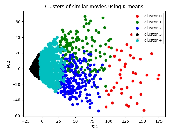
Figure 6: Clusters of similar movies
If we look at the graph, it is clear that the data points are more accurately clustered across clusters 3 and 4. However, clusters 0, 1, and 2 are more scattered and did not cluster well.
Here we did not compute any accuracy metric because train data doesn't have labels. Now let's compute the top k similar movies for a given respective movie name and print them:
ratings_df = readers.read_file("Input/ratings.dat", sep="::")
topK = main.top_k_similar_items(9,ratings_df = ratings_df,k = 10,TRAINED = False)
print(topK)
>>>
[1721, 1369, 164, 3081, 732, 348, 647, 2005, 379, 3255]
The above result computes Top-K similar movies for the movie 9::Sudden Death (1995)::Action. Now if you observe the movies.dat file, you will see that the following movies are similar to this one:
1721::Titanic (1997)::Drama|Romance
1369::I Can't Sleep (J'ai pas sommeil) (1994)::Drama|Thriller
164::Devil in a Blue Dress (1995)::Crime|Film-Noir|Mystery|Thriller
3081::Sleepy Hollow (1999)::Horror|Romance
732::Original Gangstas (1996)::Crime
348::Bullets Over Broadway (1994)::Comedy
647::Courage Under Fire (1996)::Drama|War
2005::Goonies, The (1985)::Adventure|Children's|Fantasy
379::Timecop (1994)::Action|Sci-Fi
3255::League of Their Own, A (1992)::Comedy|Drama
Now let's compute the user-user Pearson correlation. When you run this user similarity function, on the first run it will take time to give output but after that, its response is in real time:
print(main.user_similarity(1,345,ratings_df))
>>>
0.15045477803357316
Now let's compute the aspect rating given by a user for a movie:
print(main.user_rating(0,1192))
>>>
4.25545645
print(main.user_rating(0,660))
>>>
3.20203304
Let's also see the top K movie recommendations for the user:
print(main.top_k_movies([768],ratings_df,10))
>>>
{768: [2857, 2570, 607, 109, 1209, 2027, 592, 588, 2761, 479]}
print(main.top_k_movies(1198,ratings_df,10))
>>>
{1198: [2857, 1195, 259, 607, 109, 2027, 592, 857, 295, 479]}
So far, we have seen how to develop a simple RE using a movies and rating dataset. However, most recommendation problems assume that we have a consumption/rating dataset formed by a collection of (user, item, rating) tuples. This is the starting point for most variations of collaborative filtering algorithms, and they have proven to yield good results; however, in many applications, we have plenty of item metadata (tags, categories, and genres) that can be used to make better predictions.
This is one of the benefits of using FMs with feature-rich datasets, because there is a natural way in which extra features can be included in the model, and higher-order interactions can be modeled using the dimensionality parameter d (see figure 7 below for more detail).
A few recent types of research show that feature-rich datasets give better predictions: i) Xiangnan He and Tat-Seng Chua, Neural Factorization Machines for Sparse Predictive Analytics. In Proceedings of SIGIR '17, Shinjuku, Tokyo, Japan, August 07-11, 2017. ii) Jun Xiao, Hao Ye, Xiangnan He, Hanwang Zhang, Fei Wu and Tat-Seng Chua (2017) Attentional Factorization Machines: Learning the Weight of Feature Interactions via Attention Networks IJCAI, Melbourne, Australia, August 19-25, 2017.
These papers explain how to make existing data into a feature-rich dataset and how FMs were implemented on the dataset. Therefore, researchers are trying to use FMs to develop more accurate and robust REs. In the next section, we will see some examples of using FMs and some variations.