
Gradients for deeper layers are calculated as products of many gradients of activation functions in the multi-layer network. When those gradients are small or zero, it will easily vanish. On the other hand, when they are bigger than 1, it will possibly explode. So, it becomes very hard to calculate and update.
Let's explain them in more detail:
- If the weights are small, it can lead to a situation called vanishing gradients, where the gradient signal gets so small that learning either becomes very slow or stops working altogether. This is often referred to as vanishing gradients.
- If the weights in this matrix are large, it can lead to a situation where the gradient signal is so large that it can cause learning to diverge. This is often referred to as exploding gradients.
Thus, one of the major issues of RNN is the vanishing-exploding gradient problem, which directly affects performance. In fact, the backpropagation time rolls out the RNN, creating a very deep feed-forward neural network. The impossibility of getting a long-term context from the RNN is due precisely to this phenomenon: if the gradient vanishes or explodes within a few layers, the network will not be able to learn high temporal distance relationships between the data.
The next diagram shows schematically what happens: the computed and backpropagated gradient tends to decrease (or increase) at each instant of time and then, after a certain number of instants of time, the cost function tends to converge to zero (or explode to infinity).
We can get the exploding gradients by two ways. Since the purpose of activation function is to control the big changes in the network by squashing them, the weights we set must be non-negative and large. When these weights are multiplied along the layers, they cause a large change in the cost. When our neural network model is learning, the ultimate goal is to minimize the cost function and change the weights to reach the optimum cost.
For example, the cost function is the mean squared error. It is a pure convex function and the aim is to find the underlying cause of that convex. If your weights increase to a certain big amount, then the downward moment will increase and we will overshoot the optimum repeatedly and the model will never learn!
In the preceding figure, we have the following parameters:
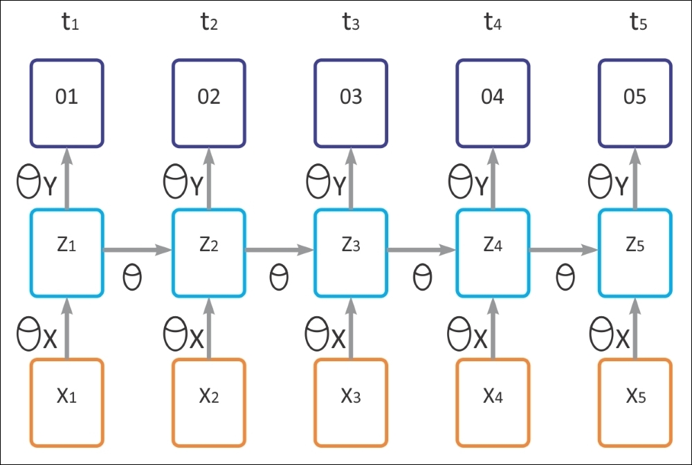
Note that the preceding diagram denotes the time lapse of the recurrent neural network model given below. Now if you recall figure 1, the output can be formulated as follows:
Now let E represent the loss at the output layer: ![]() . Then the above three equations tell us that the E depends upon the output
. Then the above three equations tell us that the E depends upon the output ![]() .Output
.Output ![]() changes with respect to the change in the hidden state of the layer (
changes with respect to the change in the hidden state of the layer (![]() ). The hidden state of the current timestep (
). The hidden state of the current timestep (![]() ) depends upon the state of the neuron at the previous timestep (
) depends upon the state of the neuron at the previous timestep (![]() ). Now the following equation will clear the concept.
). Now the following equation will clear the concept.
The rate of change of loss with respect to parameters chosen for the hidden layer = ![]() , which is a chain rule that can be formulated as follows:
, which is a chain rule that can be formulated as follows:
(I)
In the preceding equation, the term![]() is not only interesting but also useful.
is not only interesting but also useful.
(IINow let's consider t = 5 and k = 1 then
(III)
Differentiating equation (II) with respect to (![]() ) gives us:
) gives us:
(IV)
Now if we combine equation (III) and (IV), we can have the following result:
In these cases,
also changes with timestep. The above equation shows the dependency of the current state with respect to the previous states. Now let's explain the anatomy of those two equations. Say you are at a timestep five (t = 5), then k will range from one to five (k=1 to 5) this means you have to calculate k) for the following:
Now come at equation (II), each of the above
. Moreover, it is dependent on the parameter of the recurrent layer
. If your weights get large during training, which they will due to multiplications in equation (II) for each timestep (I). The problem of gradient exploding will occur.
To overcome the vanishing-exploding problem, various extensions of the basic RNN model have been proposed. LSTM networks, which will be introduced in the next section, are one of these.
One type of RNN model is LSTM. The precise implementation details of LSTM are not in the scope of this book. An LSTM is a special RNN architecture that was originally conceived by Hochreiter and Schmidhuber in 1997.
This type of neural network has been recently rediscovered in the context of deep learning because it is free from the problem of vanishing gradients and offers excellent results and performance. LSTM-based networks are ideal for the prediction and classification of temporal sequences and are replacing many traditional approaches to deep learning.
The name signifies that short-term patterns are not forgotten in the long term. An LSTM network is composed of cells (LSTM blocks) linked to each other. Each LSTM block contains three types of the gate: an input gate, an output gate, and a forget gate, which implements the functions of writing, reading, and reset on the cell memory, respectively. These gates are not binary, but analog (generally managed by a sigmoidal activation function mapped in the range [0, 1], where 0 indicates total inhibition, and 1 shows total activation).
If you consider an LSTM cell as a black box, it can be used very much like a basic cell, except it will perform much better; training will converge more quickly and it will detect long-term dependencies in the data. In TensorFlow, you can simply use BasicLSTMCell instead of BasicRNNCell:
lstm_cell = tf.nn.rnn_cell.BasicLSTMCell(num_units=n_neurons)
LSTM cells manage two state vectors, and for performance reasons, they are kept separate by default. You can change this default behavior by setting state_is_tuple=False when creating BasicLSTMCell. So, how does an LSTM cell work? The architecture of a basic LSTM cell is shown in the following diagram:
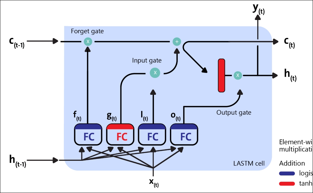
Figure 11: Block diagram of an LSTM cell
Now, let's see the mathematical notation behind this architecture. If we don't look at what's inside the LSTM box, the LSTM cell itself looks exactly like a regular memory cell, except that its state is split into two vectors, ![]() and
and ![]() :
:
 is a
is a
 as the short-term s
 as the long-term state
Now, let's open the box! The key idea is that the network can learn the following:
- What to store in the long-term state
- What to throw away
- What to read it
As the long-term![]() traverses the network from left to right, you can see that it first goes through a forget gate, dropping some memory, and then it adds some new memory via the addition operation (which adds the memory that was selected by an input gate). Theresult
traverses the network from left to right, you can see that it first goes through a forget gate, dropping some memory, and then it adds some new memory via the addition operation (which adds the memory that was selected by an input gate). Theresult ![]() is sent straight out, without any further transfo
is sent straight out, without any further transfo
Therefore, at each time step, some memory is dropped and some memory is added. Moreover, after the addition operation, the long-term state is then copied and passed through the tanh function, which produces outputs in the scale of [-1, +1].
Then the output gate filters the result. This produces the short-term ![]() (which is equal to the cell's output for this time step
(which is equal to the cell's output for this time step ![]() ). Now, let's look at where new memories come from and how the gates work. First, the current input
). Now, let's look at where new memories come from and how the gates work. First, the current input ![]() and the previous short-ter
and the previous short-ter![]() are fed to four different fully connectedThe presence of these gates allows LSTM cells to remember information for an indefinite period: in fact, if the input gate is below the activation threshold, the cell will retain the previous state, and if the current state is enabled, it will be combined with the input value. As the name suggests, the forget gate resets the current state of the cell (when its value is cleared to 0), and the output gate decides whether the value of the cell must be carried out or not.
are fed to four different fully connectedThe presence of these gates allows LSTM cells to remember information for an indefinite period: in fact, if the input gate is below the activation threshold, the cell will retain the previous state, and if the current state is enabled, it will be combined with the input value. As the name suggests, the forget gate resets the current state of the cell (when its value is cleared to 0), and the output gate decides whether the value of the cell must be carried out or not.
The following equations are used to do the LSTM computations of a cell's long-term state, its short-term state, and its output at each time step for a single instance:
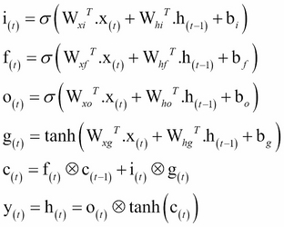
In the preceding equation, ![]() ,
, ![]() ,
, ![]() , and
, and ![]() are the weight matrices of each of the four layers for their connection to the input vector
are the weight matrices of each of the four layers for their connection to the input vector ![]() . On the other hand,
. On the other hand, ![]() ,
, ![]() ,
,
, and
are the weight matrices of each of the four layers for their connection to the previous short-term state
,
, ![]() , and
, and
are the bias terms for each of the four layers. TensorFlow initializes
to a vector full of 1's instead of 0's. This prevents it from forgetting everything at the beginning of training.
There are many other variants of the LSTM cell. One particularly popular variant is the Gated Recurrent Unit (GRU) cell. Kyunghyun Cho and others proposed the GRU cell in a 2014 paper that also introduced the autoencoder network we mentioned earlier.
Technically, a GRU cell is a simplified version of an LSTM cell where both the state vectors are merged into a single vector called ![]() . A single gate controller controls both the forget gate and the input gate. If the gate controller's output is 1, the input gate is open and the forget gate
. A single gate controller controls both the forget gate and the input gate. If the gate controller's output is 1, the input gate is open and the forget gate
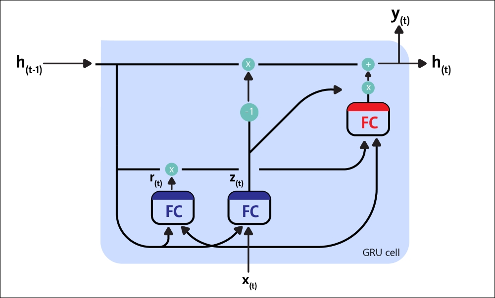
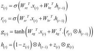
Figure 12: A GRU cell
On the other hand, if it's output is 0, the opposite happens. Whenever a memory must be stored, the location where it will be stored is erased first, which is actually a frequent variant of the LSTM cell in and of itself. The second simplification is that since the full state vector is output at every time step, there is no output gate. However, a new gate controller controls which part of the previous state will be shown to the main layer.
The following equations are used to do the GRU computations of a cell's long-term state, its short-term state, and its output at each time step for a single instance:
Creating a GRU cell in TensorFlow is straightforward. Here is an example:
gru_cell = tf.nn.rnn_cell.GRUCell(num_units=n_neurons)
These simplifications are not a weakness of this type of architecture; it seems to perform successfully. The LSTM or GRU cells are one of the main reasons behind the success of RNNs in recent years, in particular for applications in NLP.
We will see examples of using LSTM in this chapter, but the next section shows an example of using an RNN for spam/ham text classification.