
CHAPTER 19 The Salvo real-time operating system
All the concepts introduced about the RTOS (real-time operating system) in Chapter 18 are theoretical niceties unless we can apply them to a working system. Preferably, this should be one that can be run on a PIC-based embedded system. Our chance to do this comes with Salvo – ‘the RTOS that runs in tiny places’. Salvo is a commercially available RTOS specially intended for the small embedded system, with a version which works with the Microchip C18 compiler. Best of all, there is a free Salvo Lite version! This gives us the opportunity to enter the exciting yet challenging world of the RTOS, and, without too much trouble, to write simple, illustrative and working programs.
The main aim of this chapter is to provide an introduction to Salvo, to a level at which effective yet simple programs can be written. The purpose of this is to see a real RTOS applied to practical situations, rather than to become an expert user of Salvo. Therefore, the deeper detail of using Salvo is left to the user's guide.
This chapter is essentially built around three example programs, which progress through applications of key RTOS concepts. Having reached the end of the chapter, you should have a good understanding of:
19.1 The main idea – Salvo, an example RTOS
Salvo was originally developed, in Assembler, for the data-acquisition system of a racing car. Once it was recognised that it could be applied more widely, it was rewritten in C and adapted for general use. Its target application is the small embedded system. Salvo now needs to run with a C compiler; it no longer works with Assembler. Versions of it are available for many of the major embedded system compilers. Salvo is supplied by Pumpkin Real Time Software Inc.
Selected information on Salvo is given in the sections that follow; it is intended to be enough to write some interesting introductory programs. For full details on Salvo, you should refer to the supplier's reference information, notably Refs 19.1–19.3.
19.1.1 Basic Salvo features
Salvo works with a cooperative scheduler and can run multiple prioritised tasks. This is one of the keys to its low memory demands – as discussed in Section 18.4.5, cooperative scheduling is less demanding of memory. The number of tasks (in the fully featured version) is limited only by the available RAM, while 16 priority levels are available. Tasks can also share priority levels. Salvo supports a range of different ‘events’, including binary and counting semaphores, messages and message queues.
Salvo is supplied as an extensive set of files – source, header, library and others. These effectively act as extra services that are added to the host compiler. The programmer works with the host compiler in the usual way, but incorporates the Salvo files as needed. In so doing, he/she must of course follow the requirements of the Salvo RTOS. The program as developed by the programmer is finally a combination of original source code, header and source files from Salvo and the compiler, and Salvo and compiler library files. The build process and the main contributory files are summarised in Figure 19.1. The output is an executable file, which can be downloaded to program memory.

19.1.2 Salvo versions and references
There are a number of versions of Salvo available. At the de luxe end is Salvo Pro, a highly configurable, fully featured version. The freeware version of Salvo, called Salvo Lite, contains a subset of Salvo functionality. At the time of writing this may be downloaded from the Pumpkin website: http://www.pumpkininc.com/ – a copy is also available on the book's companion website. The version which matches the compiler in use, in our case the Microchip C18 compiler, must be chosen. Salvo Lite permits three tasks and five events. This sounds like a modest limit. In fact, it allows surprisingly useful and advanced programs to be developed.
Salvo comes with a big but readable user manual [Ref. 19.1]. This is written to support use of all versions of Salvo, right up to Salvo Pro. For the beginner, aiming to use Salvo Lite, some of it can be daunting. Nevertheless, it has good and informative introductory chapters. It contains all general information for the RTOS but nothing that is compiler-specific. This is contained within further reference manuals. For the Microchip C compiler the important ones are (at the time of writing) Refs 19.2 and 19.3.
19.2 Configuring the Salvo application
One of Salvo's principal features is that it is highly reconfigurable. It is therefore important early on to have a picture of how this configuration takes place. This section introduces some of the essential features of Salvo's files and configuration, and will lead to a better understanding of the build process shown in Figure 19.1.
19.2.1 Building Salvo applications – the library build
There are two main ways to build a Salvo application: ‘library build’ and ‘source-code build’. The latter requires manipulation of the Salvo source code and is for advanced players only. Anyway, it can only be undertaken with Salvo Pro, so we will not consider it here. That leaves us with library build – building the application using the library features available.
Different libraries are available for use, each one with a different set of features. For a given application, the most suitable library must be chosen. Once this is done, the library services are fixed. The user source code then makes calls to the Salvo functions contained in the chosen library.
Apart from the library files, certain other source and header files must be incorporated, as seen in Figure 19.1. The most important ones are as follows.
• salvo.h. This is Salvo's main header file and must be included in any source file that uses Salvo services. It should not be modified by the user. This file in turn includes salvocfg.h.
• mem.c. This is a major file, supplied with Salvo. It holds global objects, which define characteristics for the features used, like tasks, semaphores and so on. It should not be modified by the user, although the contents of salvocfg.h impact upon it.
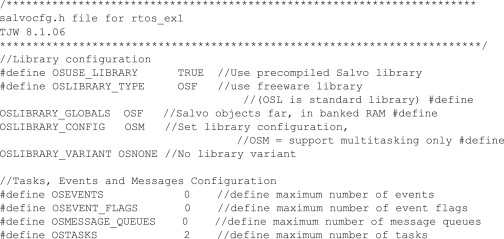
• salvocfg.h. This file, written by the user, determines much of the configuration of the system for the application. It sets certain key elements, like which library is to be used and how many tasks and events there will be. Further details are given in Section 19.4.4.
19.2.2 Salvo libraries
Salvo has a large set of standard libraries, which contain much of the RTOS functionality. There are different library sets for each compiler and different versions within compilers. These support different memory models and different combinations of features. One of the skills in configuring a Salvo application lies with selecting the library which has the features needed and nothing more.
Salvo Lite is provided with a set of freeware libraries. These are like the standard libraries, but have limited capability. The coding used for the C18 compiler is shown in Figure 19.2. The final letter of the library name indicates its ‘configuration’, which is defined in Table 19.1. The sfc18sfa.lib library, for example, has all features except time-outs. This makes it a comparatively large library. If only multi-tasking is needed in an application, it would be better to use a library with ‘m’ configuration. This would lead to more efficient coding and less memory utilisation.

TABLE 19.1 Library services available for each library configuration
| Library configuration | |||||
|---|---|---|---|---|---|
| a | d | e | m | t | |
| Multi-tasking | + | + | + | + | + |
| Delays | + | + | − | − | + |
| Events | + | − | + | − | + |
| Idling | + | + | + | − | + |
| Task priorities | + | + | + | − | + |
| Time-outs | − | − | − | − | + |
+ = enabled; − = not enabled.
19.2.3 Using Salvo with C18
When using Salvo, it is essential to ensure that a compatible combination of MPLAB IDE, C18 compiler and Salvo is used. This book uses MPLAB version 8.10, with C18 version 3.00 and Salvo version 3.2.3.c. To install Salvo, it should be downloaded from the Salvo website and the usual installation procedure followed. This is straightforward, but is detailed in Ref. 19.1 and on the book's companion website. The installation will result in the set of folders shown in Figure 19.3.

19.3 Writing Salvo programs
This section gives an introduction to programming with the Salvo RTOS, before we look at a first program example in the section which follows.
19.3.1 Initialisation and scheduling
Many of the features of the Salvo RTOS are contained within its C functions, found in the Salvo libraries. Part of the skill of programming with Salvo lies in knowing these functions and understanding what they do. Some examples, exactly the ones that will be used in our first program example, are given in Table 19.2. This gives the name of the function or service, a summary of its action and the parameters (if any) that it takes. The contents of the table will be referred to and explained repeatedly over the next few pages – do not worry if all its details are not immediately clear.
TABLE 19.2 Example core Salvo services
| Function/service | Action and parameter(s) | |
|---|---|---|
| OSInit( ) | Initialises the operating system, including data structures, pointers and counters. Must be called before any other Salvo function. No parameters. | |
| OSSched( ) | The Salvo scheduler. On every call it chooses – from those which are eligible – the next task to run. Multi-tasking can occur when this is called repeatedly. No parameters. | |
| OS_Yield( )∗ | Unconditional return to scheduler | |
| OSCreateTask(,) | Creates a task and starts it (i.e. makes it eligible). | |
| OSStartTask( ) | Makes a stopped task eligible. | |
| _OSLabel( ) | Defines a unique label required for each context switch. | |
| OSTCBP( ) | Defines a pointer to specified control block, in this case to the task control block. |
∗ Can cause a context switch.
Some of the functions shown can cause a context switch; by this means the cooperative scheduling is implemented. All Salvo functions that the user can call are prefixed with ‘OS’ or ‘OS_’. The latter is used if the service contains a conditional or unconditional context switch.
To enable and initialise the RTOS the function OSInit( ) must be called before any other Salvo function. Tasks can then be created with a call to OSCreateTask( ), ensuring that all arguments are properly specified.
The scheduler is contained within the OSSched( ) function. On every call, this does three things, as listed below:
• It processes the event queue, if events are being used. Remember, events include semaphores and messages. As a result of this, certain tasks may become eligible to run.
• It processes the delay queue, where delays in Salvo are an important means of controlling when a task executes. Again, a task may become eligible to run.
• It then selects and runs the most eligible (i.e. highest priority) task. Tasks with the same priority are run on a round-robin basis.
19.3.2 Writing Salvo tasks
Each Salvo task is written as a C function and follows the general pattern for the writing of tasks described in Section 18.5 of Chapter 18. There are further important requirements, specific to Salvo. These are summarised below:
• All tasks are initially ‘destroyed’. Tasks must be created using the Salvo OSCreateTask( ) function. They can be created anywhere in the program. In practice, many are created early in the main function.
• Tasks are generally made up of an optional initialisation followed by an infinite loop, which must contain at least one context switch.
• The context switch can be provided by a call to the function OS_Yield( ), although there are other functions which also cause a switch. With this (or equivalent) call, the task relinquishes access to the CPU and hands control back to the scheduler. This is the basis of the cooperative scheduling used by Salvo.
• Tasks use static variables; therefore, task data is unchanged when the task is not running. Variables of type auto can be used if the data does not need to be retained following a context switch.
The operating characteristics of a task are contained within its task control block (TCB). This is a block of memory allocated uniquely to the task, which contains (among other things) the task's start address, state and priority.
Tasks can, in general, follow the state diagram of Figure 18.7, with Salvo-specific interpretations of each state. These are introduced in the following pages.
19.4 A first Salvo example
A first example of a Salvo-based program is shown in Program Example 19.1. It uses the Salvo services summarised in Table 19.2. It contains just two tasks, of equal priority. One, Count_Task, increments a counter. The other, Display_Task, displays two bits of the counter value on two bits of Port C. As the Derbot hardware can be used, the two least significant bits of the counter are shifted over to the Derbot LEDs, which are on bits 5 and 6 of Port C.
19.4.1 Program overview and the main function
Looking down the program listing, this example looks at first like a regular small C program. The first indication that it is a Salvo program comes in the inclusion of salvo.h. A few lines


lower, the _OSLabel macro is applied twice. This provides a means of defining labels that are used in the task context switches. There are only two context switches in this program, one in each task. We will see that the labels chosen, Count_Task1 and Display_Task1, are applied for this purpose within the tasks.
The main function starts conventionally enough, with a little initialisation for Port C, the only port to be used. It then calls the OSInit( ) function, which initialises the operating system and sets the scene for all RTOS action to come. The tasks themselves are then created, with two calls to OSCreateTask( ). The format of this is summarised in Table 19.2, where we see that three arguments must be provided. The task start address is identified simply by the task name, from its function prototype. The TCB start address is defined using the OSTCBP( ) macro. Numbering the argument to this from one upwards allocates a TCB block to each task. Both tasks are then set to the same priority. Any value from 1 to 16 could be chosen; arbitrarily the value 10 is used. A continuous loop is then established, causing a repeated call to the scheduler OSSched( ). The action of this will be to activate the most eligible task.
Configuration bits can be set in the program in the way described in Chapter 17. The version of Salvo used leads to a small clash, however, as the name OSC is defined for two different purposes in salvo.h and p18F2420.h. Pumpkin Inc. advise that it is not needed for the C18 implementation. Therefore, it is undefined, using the #undef preprocessor directive in the line before p18F2420.h is included.
19.4.2 Tasks and scheduling
It can be seen that the tasks themselves are written as functions. Each is a continuous loop, with each loop containing an OS_Yield( ) function call. The argument to this function call is the context switch label, already defined at the top of the program. Every time the task is activated, it will execute until it reaches the OS_Yield( ) call. Here it returns control back to the scheduler, and the task moves from the ‘running’ state to the ‘ready’ or ‘eligible’ state (Figure 18.7). When the scheduler activates the task again, it picks up execution at the line immediately following the OS_Yield( ) call and returns to the ‘running’ state.
19.4.3 Creating a Salvo/C18 project
Creating a project with Salvo is initially just like creating any other C18 project. The steps outlined here are similar to those described in Ref. 19.3, where some troubleshooting advice is given as well. This is an application note for MPLAB version 6, but is reasonably applicable to version 8. At the time of writing, there is not an application note for this later version.
If you wish to build this project for yourself, and you are strongly encouraged to do so, you should start by creating an MPLAB project in the normal way. The name rtos_ex1 was used for this project. Create a folder just for this project (there will be a number of files in it), and copy to it the source file and salvocfg.h file from the folder on the book's companion website. From the salvo/lib folder, add the sfc18sfm.lib library. Also from the salvo/src folder, add the mem.c file. Your MPLAB project window should then appear as shown in Figure 19.4.
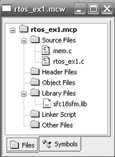
Look back at Figure 19.2 and Table 19.1 to determine the characteristics of the sfc18sfm.lib library. It should not be difficult to work out that this is a freeware library for the C18 compiler, applying the small memory model, with capability for multi-tasking only. This is an appropriate choice for this very simple program.
19.4.4 Setting the configuration file
The Salvo RTOS is configured for a particular application by the settings in the salvocfg.h file, written by the programmer. The file is made up of a series of C define statements. A limited set of these is available in Salvo Lite, while many more are available in the fully featured versions. There are default values for every configuration option, so some (or all) of these can be adopted. The more tightly the configuration file matches the actual application, however, the more efficient is the final coding likely to be. There is, for example, no point in having memory set up for six tasks when only three are required.
The salvocfg.h file used for the rtos_ex1 project is shown in Program Example 19.2. Comments are written to explain each line. It can be seen that the settings in this simple file relate either to library configuration or to program features, the latter including tasks, events and messages. The first line selects the fundamental option that pre-compiled libraries are to be used. It is important that the further library configuration options that follow actually match the library that has been selected. In this case, the sfc18sfm.lib library already selected is matched by the corresponding configuration setting, using the OSM code.
19.4.5 Building the Salvo example
A build using Salvo follows the same process as a normal C18 build. There are, however, more things which must be right for the program to build. Alongside all the possible errors of writing and linking a C program are the further requirements of a Salvo configuration. The file structure should be set up as already described and shown in Figure 19.4. The correct search path for Salvo Include Files should be specified in the Build Options dialogue box, as shown in Figure 19.5.

If the files provided on the book's companion website are applied, then a build should proceed without problems. If errors persist, it may be necessary to refer to Salvo reference material or the Salvo User Forum (at the Pumpkin website). Also check the book website (www.embedded-knowhow.co.uk).
19.4.6 Simulating the Salvo program
This first example RTOS program can be simulated just like any other. Having successfully built the program, select MPLAB SIM.
Open a Watch window, and select counter and PORTC for display. Insert the breakpoints shown in Figure 19.6. These are placed at the key points in this simple RTOS program. Then run the simulator to the first breakpoint, which is just before the RTOS initialises. Run it again, which takes you to the OSSched( ) call. A further run will move to Count_Task, which runs first as it was created first. If you single-step from here, you will see that execution remains sequentially within the task, until the OS_Yield( ) function call is reached.

Further presses of ‘run’ cause execution to alternate between tasks, visiting OSSched( ) in between each task call. Every time execution returns to a task, it picks up exactly where it left off. As the tasks are of equal priority, they are executed in round-robin scheduling.
Every time Count_Task runs, the value of counter in the Watch window increments, and every time Display_Task runs, the value of Port C is updated. In terms of functionality, we have achieved nothing startling. In terms of the way the program executes, it is a major new departure.
The program can also be run on the Derbot hardware. It is not particularly interesting to run it this way, however. As it is running at effectively uncontrolled speed, the LEDs just appear to be continuously on.
19.5 Using interrupts, delays and semaphores with Salvo
A key feature of any real-time operating system is, of course, its ability to manage real-time activity. To do this, it is more or less essential to set up a continuous ‘clock tick’, at a fixed and reliable frequency, which can be used as the time base against which other things can happen. Once the clock tick is there, many Salvo features become possible.
To establish the clock tick we need to use a timer interrupt, and we then need services to count and respond to tick-based durations. Table 19.3 gives examples of Salvo services related to interrupts and timing which we will be using.
TABLE 19.3 Example Salvo functions and services used with interrupts, timers and delays
| Function/service | Action and parameter(s) | |
|---|---|---|
| OSTimer( ) | Checks to see if any delayed or waiting tasks have timed out. If yes, they are rendered eligible. Must be called at the desired tick rate if delay, time-out or elapsed time services are required. Often placed within timer interrupt ISR.No parameters. | |
| OS_Delay(,)∗ | Causes current task to return to scheduler and delay by amount specified. Requires OSTimer( ) to be in use. | |
| OSEi( ) | Enables interrupts (sets GIE and PEIE in INTCON; see Figure 13.8). | |
| OSDi( ) | Disables interrupts. |
∗ Can cause a context switch.
19.5.1 An example program using an interrupt-based clock tick
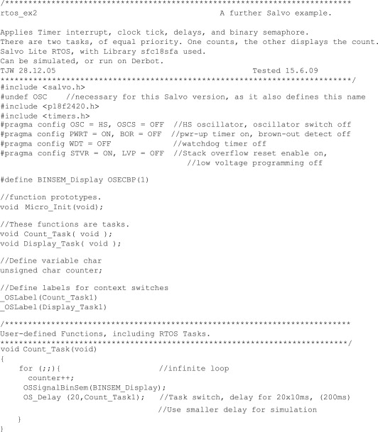
Program Example 19.3, called rtos_ex2, is a development of our first RTOS example. It keeps the same two tasks, still of equal priority, but introduces an interrupt-driven clock tick, a delay and a binary semaphore. Each of these is discussed in detail in the sections that follow. The ISR for the clock tick appears in the program example that follows.
The program is structured in a way that should be recognisable, even though new features are added. The main function initialises the microcontroller through a call to the function Micro_Init( ). This is followed by the RTOS initialisation, through a call to OSInit( ). After creating tasks and semaphore, the program enters the expected scheduling loop.

19.5.2 Selecting the library and configuration
In the rtos_ex1 example, the sfc18sfm.lib library was used. Now, however, we want to introduce delays and semaphores, the latter being a type of ‘event’. Looking at Table 19.1 tells us that the ‘m’ suffix library is no longer adequate. The best we can do is to go to an ‘a’ suffix library, even though this gives idling and priority capability, which we do not yet need.
With a different library, and new features, a new salvocfg.h file is needed for this project. This is the same as the one for rtos_ex1, except that two differences, the changed library and the inclusion of a semaphore (an ‘event’), must be identified. The lines shown below are therefore inserted in place of similar lines in the previous file. The full file is available on the book's companion website.
#define OSLIBRARY_CONFIG OSA //Set library configuration,
//OSA = support multitasking, delays & events
…
#define OSEVENTS 1 //define maximum number of events
19.5.3 Using interrupts and establishing the clock tick
Interrupts can be introduced to a Salvo-based program in the way described in Section 17.4. Program Example 19.4 shows the ISR for rtos_ex2. It follows the pattern of Program Example 17.3, except that it includes the all-important call to OSTimer( ). This function, seen in Table 19.3, allows the time-based features of Salvo to work. A variable tick_counter is also incremented on every ISR iteration. This is used in the simulation.
A clock tick period of 10 ms was chosen (somewhat arbitrarily) for this example program. It is established using the Timer 0 interrupt on overflow. This is enabled and configured through the OpenTimer0( ) call, with settings as shown in the comments. With a 4 MHz clock oscillator and the prescaler set to divide-by-16, the clock input to the timer has a period of 16 μs. Theoretically, it therefore needs 625 cycles to produce the 10 ms period. The value reloaded into the timer must therefore be 65 536 − 625, or 64 911. After the program was simulated and measurements made using the Stopwatch feature, this number was adjusted upwards to take into account the not inconsiderable interrupt latency that was observed.
The timer interrupt is enabled within the call to OpenTimer0( ). The Global Interrupt Enable is set within the call to OSEi( ), in the main function. There is nothing Salvo-specific within this macro; it is just used here for convenience.

While we have now established a useful, if not essential, clock tick feature, we need to remember that in this form it will only be approximate. The RTOS does routinely disable interrupts, for example during OSSched( ). This worsens the interrupt latency and will cause a delay in the response to the timer ISR. A timer with hardware auto-reload would give a more accurate time base. In either case, the time base formed is an approximation as, due to the cooperative scheduling, tasks can only respond to the clock tick when allowed by the action of other tasks. We will be able to assess the extent of this approximation in the simulation that is coming up.
19.5.4 Using delays
Now that we have a clock tick, we can synchronise tasks to it. One way of doing this is by using the OS_Delay( ) function, with parameters as shown in Table 19.3. This function forces a context switch when called and can thus replace OS_Yield( ). It also introduces a delay before the next time the task can run, determined by the setting of the first parameter.
The OS_Delay( ) function call is seen in the Count_Task function in Program Example 19.3, used in the following way:
OS_Delay (20,Count_Task1); //Task switch, delay for 20x10ms, (200ms)
//Use smaller delay for simulation
As the comment indicates, use of this delay causes the Count_Task function to occur periodically, every 200 ms.
19.5.5 Using a binary semaphore
The concept of the semaphore was introduced in Section 18.6. It can be used for resource protection or simply for signalling between tasks. It is a powerful feature, as it is effectively the simplest way of establishing inter-task communication. Program Example 19.3 uses a binary semaphore.
Salvo semaphores, like tasks, must first be created in the program. This allocates them an ‘event control block’ (ECB) in memory, similar to the TCB for tasks. Here, essential information on the semaphore is stored. Semaphores can then be written to by one task and waited on by another. The functions that do these three things are shown in Table 19.4.
TABLE 19.4 Example Salvo functions and services for binary semaphores
| Function | Action and parameter(s) | |
|---|---|---|
| OSCreateBinSem(,) | Creates binary semaphore. | |
| OSSignalBinSem( ) | Signals a binary semaphore. If no task is waiting it increments. If one or more tasks are waiting, then the one with highest priority is made eligible. | |
| OS_WaitBinSem(,)∗ | Task waits (in ‘wait’ state) until binary semaphore is signalled. Wait state is exited when semaphore signals and task is highest priority, or if time-out expires. Semaphore is then automatically cleared. Time-out must be specified. | |
| OSECBP( ) | Defines pointer to specified control block, in this case to the event control block. Similar to OSTCBP( ) in Table 19.2. | |
| OSNO_TIMEOUT | Entered as time-out value in OS WaitBinSem( ) if time-out is not required. |
∗ Can cause a context switch.
Our program example uses a single semaphore. As it is the only event in the program, it is allocated the ECB pointer OSECBP(1). The ECB pointer is used more than the TCB pointer in function calls, so it is worth allocating it a name. It is therefore given the name BINSEM_Display in this program line:
#define BINSEM_Display OSECBP(1)
The semaphore is created in the main function immediately after the tasks are created, in the line:
OSCreateBinSem(BINSEM_Display, 0);
This uses the ECB pointer name previously defined. The semaphore is initially set to 0.
The actual mechanics of this simple use of the binary semaphore can be understood by looking at the two tasks. Remember first of all that Count_Task only runs every 20 clock ticks, due to its use of OS_Delay(). When it runs, it signals to the semaphore through its call to OSSignalBinSem(). The action of signalling to the semaphore sets its value high. If a task is waiting for it, then that task becomes ready to run and the semaphore is cleared.
Meanwhile, Display_Task is waiting for the semaphore to go high, with the line:
OS_WaitBinSem(BINSEM_Display, 100, Display_Task1);
This indicates the name of the semaphore awaited, the time-out value and the context switch label. If no timeout is required, then a value of OSNO_TIMEOUT can be entered. The overall effect is that as soon as the count is updated in Count_Task, it is then displayed by Display_Task.
With the steps just taken, we have established simple inter-task communication and synchronisation. This is a great step forward, but there is a further advantage. A task that is waiting for a semaphore is not activated in any way by the scheduler. Hence CPU usage is made much more efficient.
19.5.6 Simulating the program
It is interesting to simulate this program and see how clock tick, tasks and the semaphore interact. Create a new project and copy the source (rtos_ex2.c), the ISR (isr.c) and the salvocfg.h files from the book's companion website. Three source files should be selected in the project window (as seen earlier in Figure 19.4): isr.c, mem.c and rtos_ex2.c. Select the sfc18sfa.lib library, ensure Build Options are set as described for Program Example 19.1, and build the program.
The following simulation settings are then suggested. Select MPLAB SIM as the Debugger and insert three breakpoints, one within each task and one in the ISR. Open a Watch window and select for display the variables shown in Figure 19.7. From the toolbar, select Debugger > Settings > Osc/Trace and set the oscillator frequency to 4 MHz. Open the Stopwatch window, as seen in the upper half of Figure 19.7, from the Debugger pull-down menu.
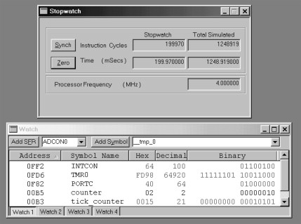
Using the simulator controls, run the program. It will halt at the first breakpoint it encounters. Assuming the timer interrupt has not yet occurred, this will be the breakpoint within Count_Task. This is the task created first, and the delay does not take effect until the first iteration of OS_Delay( ). The value of counter is incremented to 1. The semaphore is then set and a further run will reach the breakpoint in Display_Task. The value of Port C here is set by the program to 20H. The next run will find the breakpoint in the timer ISR. The time to reach the first interrupt is longer than subsequent intervals, as Timer 0 has not been preloaded and so counts up from zero.
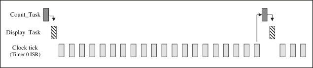
At this point, Zero the time in the Stopwatch window. Further runs will repeatedly return to the timer ISR. These are the clock ticks. It can be seen that the Stopwatch time increments by almost exactly 10 ms every time. It is interesting to note that the error is not constant, but depends on other activities of the program, which are asynchronous with the timer. This reflects the approximation discussed in Section 19.5.3. After 20 clock ticks, the Count_Task delay is up and the task is revisited. In turn it sets its semaphore and Display_Task follows. It can be seen from the Stopwatch that both of these occur comfortably within one time slice.
This general pattern of behaviour, as just described, is illustrated in Figure 19.8. This shows the broad overall sequencing of activity within the program; a precise horizontal time axis is not implied.
The two screen shots in Figure 19.7 were taken from within a program simulation. From the information given, can you deduce where program execution has halted?
19.5.7 Running the program
If you have a Derbot, download the program and run it. The LEDs will flash in a pleasing manner. As you watch this, remember: each LED change is due to an accumulation of clock ticks taking place, leading to a task being released, leading to a counter being incremented, leading to a semaphore being switched, leading to an LED display being changed. We have achieved a very simple outcome, but the elegance and power of the underlying process is extremely satisfying. This elegance and power is also available for much more challenging applications.
19.6 Using Salvo messages and increasing real-time operating system complexity
The next step we take involves learning about just one new Salvo resource, the message. This leads us, however, into a program of significantly greater complexity than the earlier ones, in which we can exercise the RTOS features in a more practical and realistic way.
Messages provide a convenient way both of transferring data between tasks and of synchronising activity between them. They have some characteristics similar to semaphores – they need to be created and can then take a piece of data from one point in the program and transfer it to another, possibly releasing a task at the same time.
Terminology with messages can be a little confusing. We can create a ‘message’ (i.e. a Salvo data-carrying structure), which can then carry any number of messages (i.e. pieces of data moved from one part of the program to another). Therefore, we call the actual Salvo service the message and then talk about ‘signalling’ the message when a piece of data is actually attached to it.
In Salvo the message signal itself can be of any data type, from character to array. The information that is actually passed is the ‘pointer’ to the signal. It is up to the programmer to ensure that this is pointing to the data required when it is signalled and that it is dereferenced properly at the receiving end. Note that a message can be sent from anywhere in the program. Thus, for example, an interrupt can signal a message, which is then received by a task.
Sample Salvo message functions and services are given in Table 19.5. These will all be applied in Program Example 19.5. As a Salvo message is a type of ‘event’, an ECB is set up for each message, just as it was for a semaphore.
TABLE 19.5 Example Salvo functions and services for messages
| Function/service | Action and parameter(s) | |
|---|---|---|
| OSCreateMsg(,) | Creates message, with ECB (event control block) pointer and initial value. | |
| OSSignalMsg(,) | Signals a message, i.e. attaches a data element to it. If more than one task is waiting for the message, then the one with highest priority is made eligible. | |
| OS_WaitMsg(,)∗ | Task waits (in ‘wait’ state) until message is signalled. Then makes message pointer (param. 2) point to it; waiting task then continues with execution. Task also continues if timed out. Time-out must be specified. | |
| OSECBP( ) | As in Table 19.4. | |
| OSNO_TIMEOUT | As in Table 19.4. | |
| OStypeMsgP | Define data type as message pointer. One of a number of predefined Salvo data types, which must be used as appropriate. |
∗ Can cause a context switch.
19.7 A program example with messages
Program Example 19.5 gives the listing of a fairly substantial Salvo-based program. It builds on the Derbot ‘blind navigation’ program of Program Example 15.3, but includes the use of an ultrasound sensor of the type described in Section 8.6.5. This was mounted pointing upwards, as shown in Figure 19.9. Note that the sensor shares port bits with the LEDs, so these are not available in this program. The program acts as the ‘blind navigation’ program, except that when the Derbot runs under an overhanging object, for example under a chair, it detects this, rotates and moves away.

The program has two tasks, now of different priorities, and two interrupts, also of different priorities. Unlike earlier examples, each task forms a substantial block of code and each contains more than one context switch. A single ‘message’ is defined; this is used to carry signals to the motor control task from both an interrupt and from the other task. A number of delays are also used.

The main function is very similar to that of the previous program example, except that a message is created instead of a semaphore.
19.7.1 Selecting the library and configuration
As far as configuration is concerned, this program is no different from the previous one. They both have two tasks and one event. In this case the event is a message. Therefore, the sfc18sfa.lib library remains the right one to use and the salvocfg.h file from rtos_ex2 can be copied in to this project.
19.7.2 The task: USnd_Task
This task periodically pulses the ultrasound sensor, to detect whether there is an overhang above the AGV. If an overhang is detected, it sends a message, which is received by the Motor_Task task. As the action of the motors depends on a measurement made in this task, it was accordingly given the higher priority.
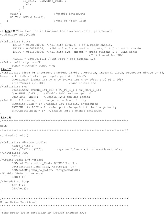
The structure of the USnd_Task is drawn from Program Example 9.7, using software delays to first generate the pulse and then to time the response. It starts from line 96 in the listing. The task uses the OS_Delay( ) function, placed at the start of its ‘infinite’ loop, to make the function occur every 20 clock ticks. When a delay period is up, it outputs a pulse by setting Port C bit 5 high, calling a delay of 20 μs and then setting it low again.
The measurement timing loop, from line 110, need be approximate only, and is only used for short-range measurement. Therefore, an effective time-out of 50 cycles is incorporated in the while loop. If the echo pulse (on Port C, bit 6) is seen to fall low during this timing loop, a message is generated. In this case the task then enters a significant delay. This uses two iterations of the OS_Delay( ) function, as it can only apply 8-bit delay values. This inhibits the ultrasound action while the Derbot turns (under the control of the other task) and moves away from the overhang that it has detected. If, however, the echo pulse does not fall low, then the timing loop simply times out and the task yields through a call to OS_Yield( ).
19.7.3 The task: Motor_ Task
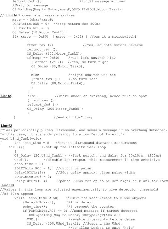
The Motor_Task task undertakes all motor settings, doing this based on the messages it receives from the Port B interrupt and the USnd_Task task. It starts from line 58 in the listing. The task opens by declaring the variable msge, where the incoming message will be stored. It then defines the message pointer msgP using a special Salvo data type OStypeMsgP (Table 19.5).
Having started the two motors, the task waits for a message to arrive, through a call to the OS_WaitMsg( ) function. Depending on the message received, execution moves to different states. As new motor states are set up, delays are forced using the OS_Delay( ) function. During waiting for both message and delay, the task is completely inactive, as it is the scheduler which initially receives the message and determines whether the task should be enabled.
19.7.4 The use of messages
Part of the power of this program lies in its use of messages. Significant lines are replicated below. In every case they make use of the services summarised in Table 19.5. Only one Salvo message, Msg_to_Motor, is created, but it is used to carry different messages from different places in the program. All are received by the Motor_Task function.
…
//Carries messages from microswitch and ultrasound
#define Msg_to_Motor OSECBP(1)
…
From main
OSCreateMsg(Msg_to_Motor, (OStypeMsgP)0);
…
From Motor_Task Function
static char msge; //hold message once recd
OStypeMsgP msgP; //Declare msgP as special Salvo pointer type
…
//Wait for message
OS_WaitMsg(Msg_to_Motor,&msgP,OSNO_TIMEOUT,Motor_Task1);
//Proceed when message arrives
msge = ∗(char∗)msgP;
…
Early in the program listing (line 50) the name of the message, Msg_to_Motor, is defined. As with the semaphore, it is actually the pointer to the ECB (event control block) which is being named, as this is used to identify the message in all three of the Salvo functions that are used.
The message is created in main using OSCreateMsg( ). Very early in the first call to Motor_Task( ), program execution reaches an OS_WaitMsg( ) call. This causes a context switch and forces the task to wait until the message identified, Msg_to_Motor, is signalled. Time-out is explicitly not applied, through use of the OSNO_TIMEOUT. The pointer for the incoming message signal is specified as msgP, which is declared at the beginning of the function.
The message is signalled from within the uswitch_isr (one example shown below) and from the USnd_Task function. The format is as shown. The predefined name, Msg_to_Motor, is again used to supply the message pointer. The value of the message signal, named Rt_usw, has been defined earlier. The pointer to the message signal is then supplied, using the special Salvo OStypeMsgP data type.
From uswitch_isr Function
…
char Rt_usw = 0x01;
…
if (PORTBbits.RB4 == 0) //Test right uswitch
OSSignalMsg(Msg_to_Motor,(OStypeMsgP)&Rt_usw); //Send message
…
19.7.5 The use of interrupts and the Interrupt Service Routines
This is the first (and only) example in the book where both a high- and a low-priority 18 Series interrupt are applied, so it is worth checking the settings. A Timer 0 interrupt is used, exactly as in Program Example 19.3, to establish a 10 ms clock tick. To this is added a Port B interrupt on change, to detect microswitch presses.
The interrupts are configured mainly at the end of the Micro_Init() function. The registers applied are seen in Figures 13.8–13.10 and the role of the IPEN bit is seen in Figure 13.7. This bit is first set high (line 147), enabling the low-priority interrupt path. In the next two lines the Port Change Interrupt is enabled and set to low priority. The Global Interrupt is enabled through the call to OSEi( ) in main.


The two ISRs are shown in Program Example 19.6. The Microswitch ISR, uswitch_isr( ), starts with a delay call of 8 ms to allow microswitch bounce to settle. Both switches are then tested. If one is found to be low, the corresponding message is generated. It is quite possible that neither is found to be low, as the ISR is called on switch release as well as switch activation. The ISR ends with the interrupt flag being cleared.
19.8 The real-time operating system overhead
This chapter has aimed to give an introduction to the power of working with an RTOS. It is important to recognise that in making use of Salvo Lite we have only used a limited subset of what Salvo has to offer, or what is available in the wider world of the RTOS.
While appreciating the power of this type of programming, it is important also to recognise the costs. These fall into three categories:
(1) Financial cost. Once we move beyond using a free RTOS like Salvo Lite or equivalent, it will be necessary to buy a commercially available RTOS or else to spend time (and hence money) in designing an RTOS from scratch.
(2) Program size cost. A program written with an RTOS tends to occupy more memory space.
(3) Execution time cost. With significantly more code to execute, due to the RTOS overheads, the program will run slower.
These costs are similar to those experienced in moving from Assembler to C programming. The programming technique is more powerful, but it comes with a cost. The last two of the above list, of course, determine the actual performance of the program. It is desirable, but not easy, to quantify these. The difficulty lies in the fact that both code size and execution time are dependent on the precise implementation of the program in question. One cannot, for example, simply say that an RTOS-based program occupies twice as much memory as a convention sequential program or runs at half the speed. A practice that is applied sometimes is to use ‘benchmark’ programs to allow comparisons to be drawn between different programming implementations of the same functional outcome.
The Salvo user manual [Ref. 19.1] has a useful chapter on ‘Performance’ (Chapter 9). This gives, in some detail, performance characteristics of the Salvo RTOS and its component parts.
As far as this book is concerned, we have a small number of programs that could be used as informal benchmarks. The Derbot ‘blind navigation’ program appeared in Assembler version as Program Example 8.4 and in C as Program Example 15.3, albeit with a different microcontroller. An interrupt-based ‘flashing LEDs’ program appeared first in a conventional C version as Program Example 17.3 and then in an RTOS-based version as Program Example 19.3. One simple comparison can be made between each of these pairs by looking at their memory usage, as seen in their. map files, described in Section 17.10.3. If you do this, you may then like to go on to explore optimising either the C or the RTOS-based versions. There is scope to do this in both cases, with some options being described in both the C compiler manual and the Salvo manual.
Summary
• Salvo is an effective real-time operating system for the small embedded environment; it illustrates in a practical way all key RTOS features and is very well suited to the PIC environment.
• Working with an RTOS leads to a new approach to programming, where tasks, priorities and events become the key features.
• There are costs associated with using the RTOS, including financial, memory space and execution time. These need to be understood and evaluated when deciding whether to use an RTOS.
19.1. Salvo – The RTOS that runs in tiny places, User Manual, Version 3.2.2. Pumpkin Inc.; http://www.pumpkininc.com
19.2. Salvo Compiler Reference Manual – Microchip MPLAB-C18 (2003, rev. 2007). Code RM-MCC18. Pumpkin Inc.; http://www.pumpkininc.com
19.3. Building a Salvo Application with Microchip's MPLAB-C18 C Compiler and MPLAB IDE v. 6 (2004). Pumpkin Inc., Application Note AN-25.2004; http://www.pumpkininc.com