
CHAPTER 16 Acquiring and using data with C
Having established a grounding in the world of embedded C, it is now appropriate to explore how C can be applied to the acquisition – and then the manipulation – of data.
The first point of interest will be to interface to the ADC peripheral with C. We will find that there are a number of useful library functions that ease this task. Having acquired some data, we will need to consider how it can be stored and manipulated. This will lead us into the field of C arrays and strings. As we will need to move data around, it will be appropriate to look at how to use the I2C peripheral. As overall this can become a complex field of study, and we are only working at an introductory level, only integer data manipulation will be considered.
As in the previous chapter, examples will mostly be applied to the Derbot-18 AGV, but all can be simulated to good effect.
At the end of the chapter, you should have a good understanding of:
• How to invoke library functions for use with the 18FXX20 ADC and I2C peripherals.
• How to invoke library functions which facilitate string manipulation.
16.1 The main idea – using C for data manipulation
One of the strengths of C lies in its ability to work with data. It defines data types, controls data movement and protects data from unwanted changes. In its use in the desktop computer environment, it has many library functions that are designed to make it easy to move blocks of data around. We will see a few of these capabilities in this chapter, applied to the embedded environment. While it has already been mentioned that we will be using only integer data in this chapter for reasons of simplicity, it is also worth stating that floating-point routines on an 8-bit microcontroller like the 18 Series are rather time-consuming in execution. This gives another reason to avoid them, except in situations where it is absolutely necessary.
16.2 Data acquisition in C
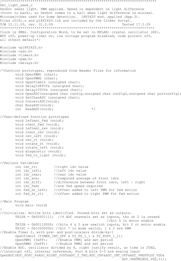
Program Example 16.1 provides a more substantial example of C programming, again for the Derbot-18 AGV. It is the light-seeking program, first introduced in Assembler as Program Example 11.3. With its three light-dependent resistors (LDRs), the Derbot seeks light, coming to a halt when all sensors are at a similar light level. The program provides useful further examples of conditional branching and introduces use of the ADC. Note that some line numbers are embedded within the comments.
16.2.1 The light-seeking program structure
With this increase in program complexity, it is useful to pause to look at the program layout. There are varied practices adopted for this; the goal of each is program clarity. The practice adopted here, where there are nested code blocks, is for the opening brace of each nested block to be indented one step to the right. Notice first the opening brace of the main function, which is fully left. Then note the position of the opening brace of the major while loop starting at line 83. This is indented one tab to the right. Further code blocks within this are indented further right again, with matching braces always lying directly below each other. The end of the while loop and end of main are both commented, and in this layout fairly easy to see. The position of a ‘fully left’ pair of braces in this book is generally reserved for the main function. Therefore, the braces for the smaller functions are indented, but still paired vertically. Major comments are given a full line or lines, while smaller comments are just placed to the right of the code.
This program, with around 20 functions, illustrates how functions proliferate as complexity increases. Around half are from the libraries, while the rest are user-defined. Function prototypes for the library functions appear in the associated header files and are thus not needed in the source file. They are, however, copied in as comments here, just for information. Prototypes for the others are included for real.
The main function starts with initialisation followed by the diagnostic function, in the usual way. The program then enters a continuous loop, making use of the while keyword. Within this it first tests the front microswitches, responding if necessary in the way seen in Program Example 15.3. It then follows broadly the flow diagram of Figure 11.13.
16.2.2 Using the 18F2420 analog-to-digital converter
The 18F2420 ADC was described in overview in Section 13.17; the C functions we can use to control it are shown in Table 14.1. Some of these are different for different 18 Series ADC versions, so it is important to choose the correct one by consulting Ref. 14.3.


This program uses all but one of the ADC functions. The most complex of these is OpenADC, whose function prototype is quoted early in the program and repeated here:
void OpenADC (unsigned char, unsigned char, unsigned char);
The three unsigned characters required as arguments are made up of bit masks, in a way similar to that described for the OpenTimer2() function in Section 15.5.1. The options for the ADC are more complex than for Timer 2. They are not reproduced here, but can easily be looked up in Ref. 14.3.
The function is used here as follows:
OpenADC (ADC_FOSC_4&ADC_RIGHT_JUST&ADC_2_TAD,ADC_CH0&ADC_INT_OFF&ADC_VREFPLUS_VDD&ADC_VREFMINUS_VSS,11);
This function makes the following settings:
• The ADC conversion speed is set. With a minimum specified conversion clock cycle time (TAD) of 0.7 μs, the 4 MHz internal oscillator is divided by four to give a TAD value of 1.0 μs.
• The result is right-justified, as seen in Figure 11.9.
• The acquisition time was calculated in Section 13.17 as 1.5 μs; this is therefore set to 2 TAD.
• Channel 0 is currently selected. This has no impact on the program that follows.
• The power supply rails are selected as the reference voltage.
• Four channels are used for input, though channel 2 is not used. This sets up the lower four bits in register ADCON1 to be 1011 (i.e. 11D), as seen in Figure 13.25.
The use of this function has the same purpose as these 16F873A Assembler lines:
bsf status,rp0
…
movlw B'10000100' ;select port A bits 0,1,3 for analog input
movwf adcon1 ;right justify result
bcf status,rp0
movlw B'01000001' ;set up ADC: clock Fosc/8, switch ADC on but not ;converting,
movwf adcon0 ;input channel selection currently irrelevant
The conversion process which follows reflects the data acquisition flow diagram of Figure 11.5. It is repeated for each LDR and appears as reproduced here, in this case for channel 0:
SetChanADC (ADC_CH0);
ConvertADC();
while (BusyADC()); //wait for conversion to complete
ldr_left = ReadADC()&0×03FF; //reverse polarity
ldr_left = 1024 - ldr_left; //reverse polarity
Here the functions used are fairly straightforward: SetChanADC() selects the input channel and the conversion is initiated with ConvertADC(). The BusyADC() function tests whether the conversion is still ongoing and returns a 1 if it is. Recall from Section 15.3.3 that a function call acts as its return value. Here the function call is embedded within the while construct. Its use causes the program to loop at that point until the conversion is complete.
The result of the conversion is then read with the ReadADC() function. The function is embedded within an expression, acting as its return value, which is the ADC result. This is a 10-bit value, with a consequent maximum possible value of 1023D. The result is ANDed with 03FFH to ensure that no higher bits are present in the reading. While this is probably an unnecessary move, it helps to illustrate how the function can be placed within an expression. Due to the hardware configuration of the LDRs, the magnitude of the result decreases with increasing light intensity. To make the subsequent arithmetic simple, the result is then subtracted from its 10-bit maximum, 1024D, so that the value of ldr_left increases with increasing light.
16.2.3 Further use of ‘if–else’
Following the data conversions, and having undertaken some intermediate calculations, the program then determines, from line 116, which (out of four) possible paths of action to take. In doing this, it is following the flow diagram of Figure 11.13. If one of the front LDRs is brightest, it will veer in that direction. If the rear LDR is brightest, it will rotate, either clockwise or anticlockwise. These decisions are made with three if–else tests, repeated below. It can be seen that the first if has an if–else nested within it, as does the corresponding else.
//determine action, by comparing LDR readings
if (ldr_left > ldr_rt)
{
if (ldr_left >ldr_rear)
fwd_left(); //ldr_left is brightest, go forward left
else rotate_left (); //rear is brightest, rotate towards light
}
else
{
if (ldr_rt >ldr_rear)
fwd_rt(); //ldr_rt is brightest, go forward right
else rotate_rt ();
}
16.2.4 Simulating the light-seeking program
It is interesting to simulate this program with the MPLAB simulator, whether or not you have a Derbot. This allows examination of the branching that is used and the operations that are applied. Set up the simulation with the following steps.
• In MPLAB, select the simulator with Debugger > Select Tool > MPLAB SIM.
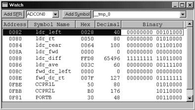
• Open a Watch window and select the variables shown in Figure 16.1 for display.
• Set up a stimulus controller and simulate inputs for the microswitch inputs, RB5 and RB4.
• Using Debugger > Settings > Osc/Trace, set the Processor Frequency to 4 MHz. This is only important here because, if set too high, the simulator is clever enough to recognise and flag that the converter cycle time, TAD (Chapter 11, Section 11.3.2), is too short.
Run the program to the first breakpoint. With the stimulus controller, ‘fire’ bits 4 and 5 of Port B to 1, to simulate the microswitches being inactive. Now run the program again to the breakpoint at line 108. The Output window will warn ‘No stimulus file attached to ADRESL for A/D’. Don't worry about this.
Now enter in the Watch window the first set of trial values, for ldr_left, ldr_right and ldr_rear, from Table 16.1. (Enter the decimal value for each and the other columns will follow.) From here, single-step through the program, using the ‘Step Into’ Debugger button. See how the correct function is chosen, fwd_to_light in this first case, and in the Watch window see the outcome of the calculations made. The results for each set of input figures are shown in the table. When you reach the first set of results, run the program back to the first breakpoint and then down to the second and enter another set of results. Continue to loop in this way, entering different trial results and observing the program response in terms of its calculations and looping.
TABLE 16.1 Trial values in the ‘light-seeking’ simulation
| Condition | Input values from ADC (decimal) | Resulting action and values (decimal) | ||||
|---|---|---|---|---|---|---|
| ldr_left | ldr_rt | ldr_rear | Function selected | fwd_dr_left | fwd_dr_rt | |
| left>right>rear | 0100 | 0080 | 0040 | fwd_to_light | 015 | 035 |
| right>left>rear | 0080 | 0100 | 0040 | fwd_to_light | 035 | 015 |
| left≫right>rear | 0200 | 0040 | 0020 | fwd_to_light | 00 | 127 |
| rear>left>right | 0080 | 0040 | 0100 | rotate_left | – | – |
| rear>right>left | 0040 | 0080 | 0100 | rotate_right | – | – |
If you have a Derbot AGV, this is an entertaining program to run. It is enhanced later in this chapter by the addition of a display capability.
16.3 Pointers, arrays and strings
We saw in Chapter 14 how data elements were declared and used. Much data exists, however, in the form of ‘sets’ of variables, for example in a string of data being prepared to send to a display. In this section we look therefore at how sets of data can be defined and used, introducing ‘arrays’ and ‘strings’, and the ‘pointers’ which access them.
16.3.1 Pointers
Instead of specifying a variable by name, we can specify its address. In C terminology such an address is called a ‘pointer.’ A pointer can be loaded with the address of a variable by using the unary operator ‘&’, like this:
my_pointer = &fred;
This loads the variable my_pointer with the ‘address’ of the variable fred; my_pointer is then said to ‘point’ to fred.
Doing things the other way round, the value of the variable pointed to by a pointer can be specified by prefixing the pointer with the ‘∗’ operator. For example, ∗my_pointer can be read as ‘the value pointed to by my_pointer’. The ∗ operator, used in this way, is sometimes called the ‘dereferencing’ or ‘indirection’ operator. The indirect value of a pointer, for example ∗my_pointer, can be used in an expression just like any other variable.
A pointer is declared by the data type it points to. Thus,
int ∗my_pointer;
indicates that my_pointer points to a variable of type int.
Reflecting the Harvard memory structure of the PIC microcontroller, the C18 compiler allows pointers to be set up both for program memory and for data memory. The resulting size of the pointer is shown in Table 16.2. The meanings of ‘near’ and ‘far’ in this context are described in Section 17.6.5 of Chapter 17.
| Pointer type | Pointer size |
|---|---|
| Data memory | 16-bit |
| Near program memory | 16-bit |
| Far program memory | 24-bit |
16.3.2 Arrays
An ‘array’ in C is defined as a set of data elements, each of which has the same type. Any data type can be used. Array elements are stored in consecutive memory locations. An array is declared with its name and data type. The number of elements can also be specified; for example, the declaration
unsigned char message1[8];
defines an array called message1, containing eight characters. Alternatively it can be left to the compiler to deduce the array length, for example in the line here:
char item1[] = "Apple";
It is easy to recognise arrays by the use of the square brackets which follow the name.
Elements within an array can be accessed with an index, starting with value 0. Therefore, for the above array, message[0] selects the first element and message[7] the last. The index can be replaced by any variable which represents the required value.
Importantly, the name of an array is set equal to the address of the initial element. Therefore, when an array name is passed in a function, what is passed is this address.
16.3.3 Using pointers with arrays
Pointers can be set up to point at arrays using the operators just introduced. For example, the statement
ADC_val_ptr = &ADC_val_BCD[0];
assigns the address of the first element of the array ADC_val_BCD to the pointer ADC_val_ptr. This assignment, if desired, can be combined with the pointer declaration itself, as follows:
int ∗ADC_val_ptr = &ADC_val_BCD[0];
Following this assignment, the value of ADC_val_BCD[0] (the first element in the array) is equal to ∗ADC_val_ptr (the value pointed to by ADC_val_ptr). It follows that the values of ADC_val_BCD[1] and ∗(ADC_val_ptr + 1) are also equal, as are ADC_val_BCD[2] and ∗(ADC_val_ptr + 2), and so on.
Because the name of the array is also its first address, the above assignment could be written as
ADC_val_ptr = ADC_val_BCD;
It follows further that ADC_val_BCD[i] is equivalent to ∗(ADC_val_BCD + i), the name of the array effectively now being used as the pointer.
A further notational development is that the pointer can be used with an index. Thus, ADC_val_ptr[i] is the same as ∗(ADC_val_ptr + i). It seems like the pointer and the array name are almost interchangeable, and that the pointer may be barely necessary. Remember, however, that the array name is a constant – the array is fixed in memory, whereas the pointer is a genuine variable, with all the properties of the variable.
16.3.4 Strings
A ‘string’ is a particular type of array, made of characters of type char, ending with the null character ‘�’. The size of the string array must therefore be at least one byte more than the string itself, to accommodate this final character.
16.3.5 An example program: using pointers, arrays and strings
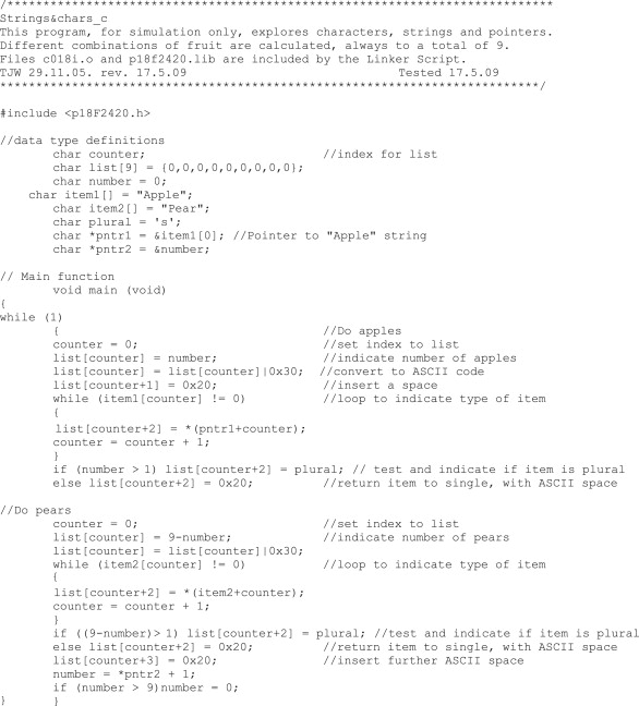
The slightly improbable Program Example 16.2 demonstrates some of the ways in which arrays, strings and pointers are used. It has nothing to do with embedded systems and is for simulation only. An array of characters, called list, is declared, with each value preset to zero. A string, called item1, is declared, containing the word ‘Apple’. A similar one is declared, with the word ‘Pear’. A single character is declared, with the name plural. Notice that strings are contained within double inverted commas and characters within a single. Two pointers are defined. The first, pntr1, is set to the address of the first element of the item1 string. The second, pntr2, is set to the address of the variable number.
16.3.6 A word on evaluating the ‘while’ condition
The while keyword was introduced in Section 14.2.8 of Chapter 14. While we have used it a number of times for endless loops, this is the first time that we use it in a conditional sense, in the line:
while (item1[counter] != 0) //indicate type of item
There is a similar usage a few lines later. Here we have spelled out the condition for looping: that the array element identified by the value of counter must not be equal to zero. We can in fact simplify this, as was explained in Chapter 14. The loop will continue executing as long as the conditional expression is ‘true’ (i.e. non-zero) and will be left when the expression is zero. Therefore, a simpler way of writing the while statement is:
while (item1[counter]) //indicate type of item
This will have an effect in the program identical to the original version of the line.
16.3.7 Simulating the program example
Create a project round Program Example 16.2 (the source code is on the book’s companion website), build it and simulate with the MPLAB simulator.
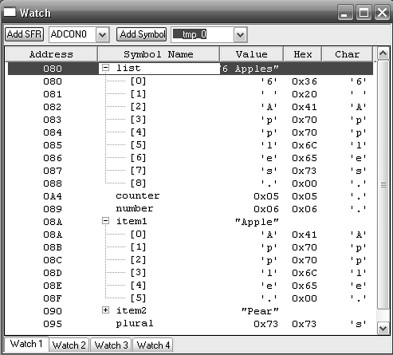
Open a Watch window, showing the variables seen in Figure 16.2. This gives an opportunity to see how the simulator handles the display of arrays. The figure shows that they can be displayed by name only, as with item2, or they can be expanded to a full listing, as with list and item1. Notice that item1 has been created with six elements, the last one being a null character which the compiler has inserted.
Set breakpoints at the locations shown in Figure 16.3 and run the program down to the first. Then single step carefully through the program, noting the action of each line. There are two program sections, identified by the comments ‘Do apples’ and ‘Do pears’. The action of each section is essentially to populate the array list with a number and the type of commodity, i.e. apple or pear.

After initialising counter, the number is transferred to the first location in the array, with the line
list[counter] = number; //indicate number of items
This uses the simplest form of array accessing, where the number contained in the square brackets indicates the array element. In this case, the first element of the array is assigned the value number. The following line converts this to ASCII code, by ORing with 30H. An ASCII space is then inserted.
A while loop is now set up. A string is known to terminate with a null character, so a test is made for this. The ‘not equal to’ operator is used in this line:
while (item1[counter] != 0) //indicate type of item
As long as the character is not null, it is transferred from the string item1 to the array list, in this line:
list[counter+2] = ∗(pntr1+counter);
The list element is again determined with an index in the squared bracket. Now the value of counter is offset by two, as its first two elements are already populated. The value assigned to it is the indirect value of pntr1, offset by the value of counter. When the end of the string has been reached, a test follows for whether the number of apples is greater than one. If so, an ‘s'must be added to the commodity type. Otherwise, a space is inserted.
Notice that in the ‘Pears’ section of the program, the string is transferred in a different way. Now the array element in the item2 string is determined using the array name as the base address, offset in turn by the value of counter. It is the indirect value of this calculated address which is transferred to the list.
Towards the end of the loop the value of number is incremented. On the right-hand side of the assignment, number is accessed by using the indirect value of its pointer, i.e. number itself.
number = ∗pntr2 + 1;
Single-step through this program until you understand what each line of code is doing. Then run it from breakpoint to breakpoint and see how the contents of the list array updates in each loop iteration.
One thing may strike you as a little odd – that the strings we have defined have found their way into data memory, as the Watch window indicates. Normally, we expect to find such strings in program memory. We return to this issue in the next chapter, when we explore how it is possible to control in which memory type strings and other constants are placed.
16.4 Using the Inter-Integrated Circuit peripheral
We saw in Chapter 8 that I2C is a useful standard for serial communication, but with some complexity in use. The C18 compiler library provides us with some very useful functions, which allow most I2C functionality to be implemented in a simple and reliable way. Reference 14.3 lists no less than 15 functions for use with I2C, although some are synonyms of others. Examples are shown in Table 16.3 in the order in which they might be used.
TABLE 16.3 Example Inter-Integrated Circuit library functions
| Function | Action |
|---|---|
| OpenI2C( ) | Configures the SSP module for I2C |
| StartI2C( ) | Generates an I2C Start condition |
| WriteI2C( ) | Writes a single byte to the I2C |
| ReadI2C( ) | Reads a single byte from the I2C |
| StopI2C( ) | Generates an I2C Stop condition |
16.4.1 An example Inter-Integrated Circuit program
A simple program which uses the I2C microcontroller capability, and applies the functions of Table 16.3, is shown in Program Example 16.3. The program is intended for the Derbot AGV and sends a single character, followed by a string, to the hand controller.
Program Example 16.3 Using an Inter-Integrated Circuit to send a character and string to the Derbot hand controller
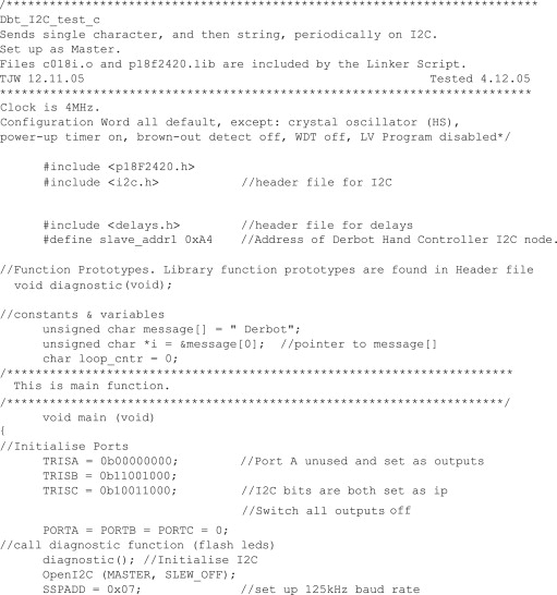
The opening lines of the program indicate which header files are to be included and define A4h as being the address of the hand controller slave node, as described in Section 10.8 of Chapter 10. They also declare the character string which forms the message that is to be sent and declare a pointer for it.
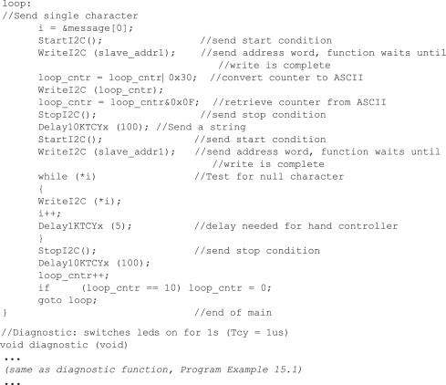
The I2C port is partially initialised with the OpenI2C() function. This has two arguments, detailed in Ref. 14.3, which determine the operating mode (whether Slave or Master) and select the slew rate. Note that it is still necessary to set the baud rate by writing to the SSPADD register. An I2C message is initiated with the StartI2C() function, which puts an I2C Start condition on the serial link. This is followed by the address byte being sent, being passed as an argument to the WriteI2C() function. This sets the R/W bit in the transmitted word low, as seen in Figure 10.13. The ASCII version of the loop counter value is formed, which is then sent through another use of the WriteI2C() function. The message is terminated with a StopI2C() function.
The string is sent by techniques which are mainly familiar, although certain developments of these are applied. A new I2C message is initiated with the StartI2C() function, followed by another sending of the slave address. A while loop is then set up, with the condition
while (∗i)
With i as the pointer to the string, ∗i indicates an element of the string. Remembering that the last string element is always a null character, the loop will be repeated until the end is reached, whereupon it will be exited.
16.4.2 Use of ++ and – – operators
Towards the end of the program example we see the ++ operator applied to both the index i and to loop_cntr. The operator, which causes an increment to the variable to which it is applied, can be seen in Table A6.5. Therefore,
There are, however, some important differences. This operator can be placed before the variable, in which case it indicates ‘pre-increment’. If it is placed after the variable, it indicates ‘post-increment’. The difference is not of significance in this program. It can, however, be understood by looking at these two examples:
index = 4; index = 4;
new_val = index++; new_val = ++index;
In the example on the left, new_val takes the value 4 and index is then incremented. In the example on the right, index is (pre-)incremented and new_val then takes the value 5.
The decrement operator, – –, is applied in exactly the same way.
16.5 Formatting data for display
We have seen now how characters and character strings can be sent over an I2C link to an LCD display. What we have not yet done is generate some meaningful data to be displayed. This section develops the Derbot ‘light-seeking’ program (Program Example 16.1), so that the values read by the light-dependent resistors are shown on the hand controller display.
16.5.1 Overview of example program
In Program Example 16.1, values are read from the ADC as 10-bit numbers. To convert this to a character string we need to convert the value to BCD and then to ASCII. We did this in Assembler, in Program Example 11.2, and very laborious it proved to be. Can C work better for us?
The answer to this question is a resounding ‘yes’. C has many functions that are designed to convert data from one format to another. A few examples are shown in Table 14.3. What we need for this application is a function that will take our 10-bit ADC output and convert it into a character string. This is very conveniently provided by the function itoa (read this as i-to-a – integer to ASCII), seen in the table.
Program Example 16.4 shows sections of the program light_seek_&_disp, which appears in full on the book’s companion website. The sections shown are extensions to Program Example 16.1. Two new functions have been written. One, disp_int(), formats the ADC output value and sends the resulting character string on the I2C link. The other, send_space(), simply sends a series of spaces to the display, to optimise information layout on the LCD.
The data is displayed only once every 10 iterations of the main loop. To do it any faster makes the data flicker in an annoying way. A loop counter, loop_cntr, has been inserted in the main loop and is incremented for every loop iteration. When data is to be displayed, it can be seen that disp_int() is called three times, once for each of the LDRs. These two results will be placed on the first line of the two-line display. Spaces are sent before and after the display of the rear LDR to centre it on the second display line.
16.5.2 Using library functions for data formatting
Let's take a close look at the function disp_int(), in Program Example 16.4, as it includes some important features. Notice first that an array, a pointer and a character variable are declared at the beginning. These will exist only for the duration of the function. The array is set for five locations, as the maximum digit count from a 10-bit number will be four (1023D) and a fifth byte is needed for the terminating null character. The argument transferred to the function is labelled op_int. The pointer is initialised to point to the start of the array.
The itoa() function is then called. This has the function prototype:
char ∗ itoa (int value,char ∗ string);
where value is the integer to be converted, string is the string where the result is to be placed and the return value is the pointer to the string. Its implementation is in the line:
itoa (op_int, disp_val_ptr);//first convert to a BCD string
It can be seen that op_int is the variable to be converted and that the resulting string is to be placed, by use of its previously declared pointer disp_val_ptr, in the array disp_val.
It would seem that this character string could be sent straight away to the display. It may, however, be of any length from one to four digits. To ensure that it always occupies the same location on the display, it is necessary first to find out how long it is. This is done with the strlen() function, found in the general software library. The function measures the length of a string and returns its value. Its prototype is:
size_t strlen(const char ∗string);
Here string is the string to be measured and the return value, size_t, contains the string length. The function is used to compute a value for space_no, which holds the number of spaces
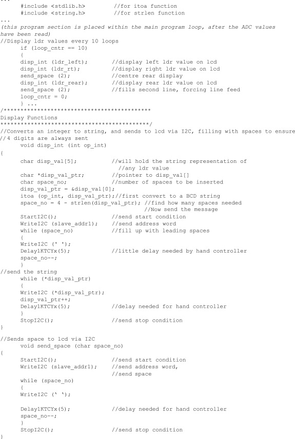
which must be sent to make up the value to four digits. These are sent before the data itself. The string is then sent and the function terminates.
16.5.3 Program evaluation
This program combines the function of the earlier light meter (Program Example 11.2) and light-seeking programs in one. It can be simulated in a similar way to that described in Section 16.2.4, inserting trial values into ldr_left, ldr_rt and ldr_rear, observing their conversion to a string and the string length being tested.
It is also a very satisfying program to run on the Derbot, as both its action and the data displayed provide a very explicit demonstration of what the program is doing.
Summary
This chapter aimed to show how C can be applied in acquiring and using integer data in embedded systems. The main points were:
• The 18FXX20 ADC and the I2C serial port can be driven in a straightforward way using library functions.
• Arrays and strings, with their associated pointers, provide powerful ways of dealing with sets of data. Some care is needed in understanding the way C deals with these.
• There are a number of library functions for manipulating data strings. These are particularly useful for formatting data in readiness for display.