
3
Systems Thinking and System Dynamics: A Primer
Brian Dangerfield
Salford Business School, University of Salford, UK
3.1 Introduction
This chapter introduces the basics of the system dynamics simulation methodology, together with the adjunct field of systems thinking which emerged subsequently. The field of system dynamics was initially known as industrial dynamics, which reflected its origins in the simulation of industrial supply chain problems. The first paper published by the founder of the field, Jay W. Forrester, appeared in 1958 (Forrester, 1958) and it was a precursor to what proved to be a hugely influential book: Industrial Dynamics (Forrester, 1961). Forrester sought to apply concepts of control engineering to management-type problems and was very probably influenced by the earlier work of Arnold Tustin (Tustin, 1953). Forrester argued that the field of operations/operational research (OR) at that time was not focused on the sort of problems that sought to inform policy (top-level) issues in an organisation. By its very definition OR was restricted to operational problems. Forrester saw a niche for a methodology which could tackle strategic issues more appropriately addressed to the success or failure of an organisation, as well as prominent national and international policy issues. See Forrester (2007) for his personal recollections of the history of the field.
The characteristics of system dynamics1 models can be listed as follows:
- They address issues by considering aggregates (of products, people, etc.) and not individual entities (as in discrete-event simulation – see Chapter 2) or individual agents (as in agent-based modelling – see Chapter 12).
- They primarily reflect the dynamics of a system as having endogenous causes: change over time comes from within the system boundary due to information feedback effects and component interactions, although the initial stimulus for those dynamics may be exogenous. For more on the endogenous perspective see Richardson (2011).
- They carefully distinguish between resource flows and the information flows which cause those resource flows to increase or run down. This is a fundamental (and powerful) feature of the methodology, which means such models can be used to design and evaluate information systems as well as the more usual focus on resource systems.
- The flows are assumed to be continuous and are governed by what are in effect ordinary differential equations. System dynamics (SD) models belong to the broader category of continuous simulation models.
- Although flow rates are included, SD models are primarily concerned with the behaviour of stocks or accumulations in the system. These are described by integral equations. Forrester has famously stated that differentiation does not exist in nature, only integration. Mathematical models characterised by differential equations must be solved in order to determine the stock values; system dynamics puts stock variables to the forefront.2
- They do not ignore soft variables (such as morale or reputation) where these are known to have a causative influence in the system.
Before addressing some of these characteristics in greater detail it is sensible to offer an overview of the adjunct field of systems thinking. This is sometimes described as qualitative system dynamics for its provenance is based upon diagramming or mapping techniques, primarily influence diagrams or causal loop diagrams. It was not until the 1970s, nearly 15 years after the publication of Forrester's early industrial models, that such diagrams started to appear. Their origins can be traced back to Maruyama (1963); the text by Goodman (1974) portrays some seminal examples.
3.2 Systems Thinking
The use of diagramming techniques in the analysis of a system has a long history going back to the block diagrams of control and electrical engineering. However, the qualitative strand associated with SD emphasises the feedback loops present in the system. Feedback is an essential building block of SD whereby information about the current state of the system is used to regulate controls on the resource flows and it underscores the endogenous point of view. For instance, if stocks of manufactured goods are beginning to over-accumulate, it is necessary either to cut back on production throughput or to inaugurate a sales drive, or both.
These mapping techniques are not mandatory in an SD study. On the other hand there are those who argue such methods, of themselves, have the capacity to generate insight and can help form a consensus for policy change in a problem system. See for instance the testimony from Merrill et al. (2013) concerning a health application. They state: ‘As a tool for strategic thinking on complicated and intense processes, qualitative models can be produced with fewer resources than a full simulation, yet still provide insights that are timely and relevant.’ Books have appeared which focus exclusively on such mapping techniques, for instance Ballé (1994) and Sherwood (2002), to the exclusion of formal simulation models which are described in Section 3.3 below. Whether such diagrams alone can be considered advantageous in the overall practice of SD has long been the subject of debate in the field. An exchange between Coyle and Homer and Oliva occupied many pages of the System Dynamics Review in 2000–2001. See Coyle (2000, 2001) and Homer and Oliva (2001).
Although the proponents of the need for formal SD models remain implacable, some authors and organisations have prospered in the propagation of systems thinking techniques. Pegasus Communications (now Leverage Networks) has for many years published the magazine The Systems Thinker and Peter Senge's reputation as a managerial thought leader was founded on his book The Fifth Discipline (Senge, 1990) and its associated Fieldbook (Senge et al., 1994). It was these sources that, primarily, introduced ‘behaviour over time’ sketch graphs together with the notion of system archetypes as additional tools in the armoury of systems thinking.
3.2.1 ‘Behaviour Over Time’ Graphs
Consider the chart in Figure 3.1. It represents some (hypothetical) data for two local authorities showing the percentage of girls who were classed as overweight in 2012.
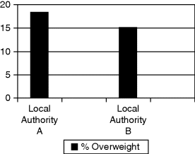
Figure 3.1 Prevalence of overweight girls aged 10–15 years in two local authorities in 2012.
It is a static graph and, as such, conveys limited and what could be misleading information. At first, an examination of the data would appear to suggest that local authority A has a more serious public health situation on its hands than local authority B. However, reframing the situation using a ‘behaviour over time’ graph paints an altogether different picture (see Figure 3.2). It is clear that local authority B is more in need of a public health intervention. Consideration of the dynamics in a system is vitally important.
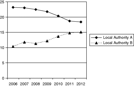
Figure 3.2 ‘Behaviour over time’ graph of the prevalence (%) of overweight girls, 2006–2012.
3.2.2 Archetypes
System archetypes are particular configurations that are capable of being expressed as a mapping in the form of an influence diagram. They commonly recur in various real-world situations and are accorded short descriptors. Besides the reference to Senge above, Wolstenholme (2003) has also contributed to the seminal literature on archetypes.
A classic archetype is the ‘tragedy of the commons’ which was first described by Hardin (1968). It accounts for how the behaviour of herdsmen in medieval England sowed the seeds of their own misfortune. Each would gain increased utility by purchasing another beast. But their actions, taken collectively, resulted in overgrazing to such an extent that the common land could not support such a large total herd – and many animals died of starvation. Today, many instances of this archetype abound, a notable example being the excessive exploitation of a common fishery. This was the basis for the well-known ‘FishBanks’ simulator game in SD (Meadows and Sterman, 2012).
3.2.3 Principles of Influence (or Causal Loop) Diagrams
This section examines the building blocks of the mappings which have come to constitute the heart of systems thinking – the diagrams known as influence diagrams (IDs) or causal loop diagrams (CLDs). There is no counterpart to an ID or CLD in discrete-event simulation. There one progresses to the development of an activity cycle diagram as the initial framework on which the computer simulation model is constructed. That is to say, the field of discrete-event simulation does not offer an optional diagramming phase which, of itself, is capable of generating insight.
Some practitioners have expressed the view that, in certain instances, an intervention based on systems thinking diagrams is sufficient to unearth the insight necessary to achieve a profound effect on system performance. The argument is bound up with project resources: models as mappings absorb less costs and can still produce insights which are timely and relevant.
A simple example of an influence diagram is given in Figure 3.3. Here we see the basic process underlying a firm's organic growth. As average profits increase they are reinvested to the future benefit of the organisation (positive links).
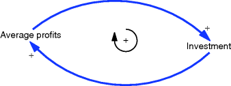
Figure 3.3 Simple positive feedback loop. (Note that the loop descriptor in the middle should flow in the same direction as the loop, in this case clockwise.)
Other examples of positive links are: sales per unit time of a durable product increase the customer base; revenues received increase the cash balance; students enrolling on a course increase the total student population.
Note that the + sign implies not only that an increase in one variable causes an increase in another, but also, alternatively, that a reduction in one variable causes a reduction in another. In the example in Figure 3.3 a reduction in average profits engenders a reduction in investment. A more obvious example is when rumours of a firm's financial health lead prospective customers to decline to engage with it.
Let us now consider a negative loop. The underlying influence created by such a loop is one of a controller. If movement occurs in the dynamics in one direction then a countervailing force pushes against that momentum to establish the original (or a new) equilibrium. The entire discipline of control engineering is concerned with how negative loops can be represented as physical controllers in machinery of all types, for example the autopilot in modern aircraft and the thermostat in a heating system.
Figure 3.4 shows an example of a simple negative loop taken from the domain of stock control. The very word ‘control’ reflects the nature of what is going on. As stock levels increase then replenishment ordering is cut, or vice versa (negative link). The change in the flow of orders directly affects the stock level and thus completes the loop. Other examples of negative links are: a perceived reduction in the numbers of a particular workforce will lead to an increase in employee recruitment; an increase in spending on wages will lead to a fall in an organisation's cash balances.
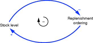
Figure 3.4 Simple negative feedback loop.
In selecting the sign to place on a given arrowhead (establishing link polarity)3 it is important not to take into account other influences that may be simultaneously operating. The Latin maxim of ceteris paribus, so common in elementary economics texts, needs to be adhered to: that is, let other factors remain constant. Therefore the only consideration in assigning link polarity is: what effect will a change in the variable at the tail of the arrow have on the variable at its head?
Two mutually connected negative relationships create a positive loop. Consider Figure 3.5 where an increase in staff turnover (in a close working team) will lead to a fall in morale which in turn will lead to a further increase in staff turnover.
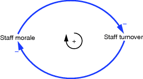
Figure 3.5 Two mutually causative negative relationships create a positive loop.
In determining the loop (as opposed to link) polarity there are two methods available. One can enter the loop at any given point, and start with, say, an increase in that variable and trace around the effect. If one returns to that point with a further increase then the loop is positive, but if the initial increase has resulted in a decrease then the loop is negative. An arguably easier approach is to add up the number of negative links in the loop: if the number is zero or is even, then the loop is positive; if it is an odd number, then the loop is negative. The loop polarity is the algebraic product of the number of negative signs, for example three negatives multiplied together yield a negative result, hence a negative loop.
3.2.4 From Diagrams to Behaviour
The determination of loop polarity is not merely an exercise for its own benefit but rather serves as a precursor to being able to infer the behaviour mode of the loop if it were to be ‘brought to life’. Loop dynamics differ between negative and positive loops so it is essential to determine loop polarity. A positive loop produces dynamics which reinforce an initial change from an equilibrium point and so underpin growth and decay behaviour patterns. A pure positive loop in growth mode will produce exponentially increasing behaviour. A negative loop, on the other hand, will generate equilibrating behaviour such that any shift away from an initial equilibrium point will produce a compensating force driving it back towards that point (or indeed a new equilibrium). Introducing a delay into a negative loop will induce an oscillation in the behaviour. It is this knowledge which can aid in model conceptualisation when time series data is available. After smoothing out any noise which may be present, an oscillatory behaviour pattern is indicative of a system dominated by a negative loop or loops; one which exhibits growth or decay would suggest that a positive loop is at work somewhere. An oscillatory behaviour associated with a trend up or down would suggest the need for a model conceptualisation based around a combination of negative and positive loops.
In order to further develop this idea of behaviour generated by different feedback loops it is necessary to move away from the single loop examples above to a more realistic real-world situation where multiple loops are at play. For instance, the example in Figure 3.6 portrays a simple product diffusion model where initial sales generate further growth through ‘word-of-mouth’ effects but this growth is ultimately curtailed by market limitations of one form or another. Because this system structure also underpins the dynamics of an epidemic in a closed population (e.g. passengers on a cruise liner), the variables named for the diffusion example have been duplicated by the equivalent epidemic variables: the same system structure can underpin quite widely different situations!
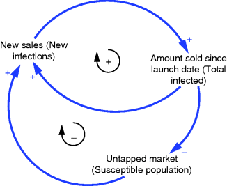
Figure 3.6 Influence diagram showing two loops and two different examples: diffusion dynamics and epidemics underpinned by the same system structure.
Also brought out by Figure 3.6 is the associated concept of loop dominance. As the structure plays out over time, the positive loop is dominant initially – that is to say, it has the control of system behaviour in the early stages while the word-of-mouth effects are at play. Ultimately the market limits begin to take over. There are fewer and fewer people who do not have this product and so the capability of making further new sales is diminishing by each passing week. Now the negative loop assumes dominance in system behaviour and growth slows. Figure 3.7 shows the resultant behaviour: S-shaped growth where the transition from growth to market maturity coincides with the switch in loop dominance. Technically this is at the point of inflection on the cumulative curve, a point where the sales per unit time (not shown) reach a peak and start to fall.
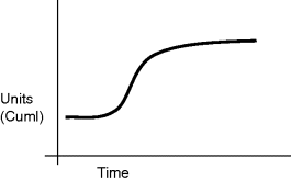
Figure 3.7 S-shaped (or sigmoidal) growth generated by coupled positive and negative loops.
3.3 System Dynamics
It is now appropriate to move forward and to consider the conceptualisation and formulation of a formal SD simulation model. As mentioned earlier, there is no essential requirement to preface the creation of an SD model with an influence diagram. There are those who argue that an influence diagram can aid in the definition of system content (and model boundary), but there is no direct linkage between such a diagram and the formal simulation model. This is in contrast to the stock–flow diagram: here the stocks (levels) and flows (rates) need to be explicitly present in the equation listing for the model.
3.3.1 Principles of Stock–Flow Diagramming
The stock–flow diagram in SD is the counterpart to the activity cycle diagram (ACD) in discrete-event simulation (DES). Although the flows may not result in a cycling of resources as such (which is common in DES), each diagram is there to underpin the formal model and the quantitative expressions which define its constituent elements.
SD flow rates are depicted by a tap-like symbol which indicates a device that can control the flow, equivalent to policy controls in the real world. A stock is represented by a rectangle and here there exists an unfortunate misalignment in the DES and SD diagramming conventions. In DES a rectangle is reserved for an activity – an active state. A stock in SD is a ‘dead’ state, equivalent to a queue in DES. Figure 3.8 is an example of what might be part of the stock–flow diagram underpinning an SD model of a nation's education system.

Figure 3.8 Example of a single flow process in a stock–flow diagram.
It is important to note that the boundary of the flow at each edge of the system is represented by a cloud-like symbol. Consideration of the resource beyond these points is outside the scope of the model. Also the stocks and flows must alternate along the sequence. The incoming flow adds to a stock while an outgoing one drains it. Only one resource can be considered along any process flow. So, for example, what starts as a flow of material (or product) cannot suddenly be transformed into a flow of finance. Thus, separate flow lines need to be formulated for the various different resources being considered in the model. ‘Resource’ can be taken to be a product class, financial flow, human resources, orders, capital equipment, and so on. Clearly the more resource flows being considered, the more complex the model and the more equations it will comprise.
Further possible arrangements are shown in Figures 3.9 and 3.10. One can have an inflow to a stock without an outflow (or vice versa). It is possible to have more than one inflow and/or outflow as in the example of the financial flows into and out of a state treasury department. In certain cases the flow might actually form a cycle. This can happen, for instance, if one is modelling a manufacturing recycling process often described as ‘reverse logistics’ or a ‘closed loop supply chain’. Although such flow arrangements do constitute a loop or cycle they are in no circumstances a feedback loop. As will be described later, a feedback loop is based on information feedback.

Figure 3.9 An inflow without an outflow.
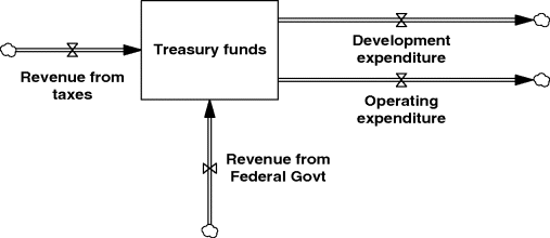
Figure 3.10 Multiple inflows and outflows in a stock–flow diagram.
3.3.2 Model Purpose and Model Conceptualisation
Getting started can be the greatest difficulty in the creation of a useful SD model. One starts with the proverbial blank sheet of paper. Experience over many years has taught the author that two fundamental aspects of SD model conceptualisation are: first, being able to write in one sentence the purpose of the model; and, second, ensuring the stock–flow representation is ‘right’. This latter term is deliberately placed within inverted commas because no model can ever be perfectly correct and represent the ultimate truth, but it is meant to suggest that a great deal of thought needs to go into deciding which resource flows to include, and how to structure those flows as bald stocks and flows with no consideration of any other variables or constants at this juncture – these can be usefully termed the spinal stock–flow structures (see examples in Figures 3.8–3.10). Where clients are involved they need to ‘buy into’ that raw stock–flow diagram and the written definition of model purpose before any further model formulation work is undertaken. Several iterations of this first conceptualisation are typically necessary. The above advice also underlines the point made earlier about influence diagrams – they are not always necessary as a precursor to formal model creation. For this task the stock–flow diagram reigns supreme.
A particularly useful precept, first expressed by Forrester in Industrial Dynamics (1961), is to define the level (stock) variables. These would still be visible if the system metaphorically stopped (e.g. employees in a factory, cash in the firm's bank accounts). Next, consider what might be flowing into and/or out of those stocks. These flows would, of course, not be visible if the system ‘stopped’. All the time it is necessary to remember that a number of different spinal stock–flow modules may be required in order to fully conceptualise the model in line with the agreed model purpose.
3.3.3 Adding Auxiliaries, Parameters and Information Links to the Spinal Stock–Flow Structure
In order to flesh out the spinal stock–flow structure it is necessary to embellish it with other explanatory variables (called auxiliaries), together with parameters. In general one follows the oft-restated mantra: rates (flows) affect levels (stocks) via resource flows, while levels (stocks) affect rates via information (feedback) links. The sequence is:
- Resource flows
 System state
 - System state Information to management
- Information to management Managerial action
- Managerial action Resource flows.
This is the essential expansion of the concept of the feedback loop which is illustrated in Figure 3.11.
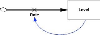
Figure 3.11 A simple feedback loop in stock–flow symbolism.
In general, more complexity will be required and other variables, which are neither stocks nor flows, of necessity have to be introduced – these are termed auxiliaries. These reflect variables which, in a business model, lie in the managerial planning and information system. Thus any variable which is intended to represent something planned, desired, a target, or a management goal would be modelled by an auxiliary variable. Consider the augmented stock–flow diagram in Figure 3.12. Here the concept of a desired workforce has been added to explain the recruitment rate on the spinal flow. It would seem intuitive that recruitment policy might be explained by a comparison between the desired workforce and what one currently possessed.
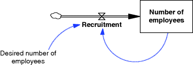
Figure 3.12 Auxiliary variable and information links added to the spinal flow.
The level of sophistication can increase, however. To jump ahead a little, there is another item which would need to be added, namely the adjustment time for eliminating any discrepancy between the desired and actual workforce. Workforce adjustment time would be a parameter and would mimic the average time to advertise and recruit new people or to give notice of redundancy and fire them if business conditions dictated it. Moreover, it might be necessary to have two different parameter values if the average time constant were thought to be different for recruitment and firing processes. Additionally, there may be a need to introduce other auxiliary variables in order to better define the desired number of employees. In fact chains of auxiliaries are often created in order to effect a proper definition for the flow variable. SD models tend to reflect real-world causes and effects very closely and this is one of the reasons why it is such a powerful methodology and why the total number of variables and parameters can rapidly escalate over and above the original number of variables on the spinal flows.
3.3.4 Equation Writing and Dimensional Checking
Undoubtedly for many the most challenging task in SD model formulation is the composition of the equations for the rates and auxiliary variables. In modern SD software the stock variables are automatically created because the system can ‘see’ what is flowing into and/or out of a stock. These integration equations take the form
SD simulations exhibit a constant time advance (unlike DES) and through this process the equations describing the flow rates (which are, in effect, differential equations) are converted to difference equations and solved to yield the values of the stocks as in the example above. In the earlier SD literature the time increment was termed dt to reflect the ‘with respect to’ element commonly seen in differential calculus; TIME STEP is often employed nowadays. Its value is normally restricted to a binary fraction (1/2n, for n = 0,1,2…) because of the way computers handle real numbers; by this means the greatest accuracy is achieved in determining the value for the system (reserved) variable Time. Clearly at the beginning of the simulation an ‘old’ value is needed to initialise the stock and this is termed an initial value. All stocks must have an associated initial value declared in order for the time advance process of the simulation to get started.
However, while formulation of the integration equations can be left to the software, this is not the case with rate and auxiliary equations. Here the user needs to compose the expression based upon the known informational influences evident in the developing stock–flow diagram. To this end it is recommended that the influence links are entered on the diagram before building the equation.
Structuring the equation is unavoidably bound up with units (or dimensional) checking. Most with a background in the physical sciences and engineering will know that any equation describing a real-world process needs to have the units balanced on each side of the ‘=’ sign. Thus, if the units on the left are $/yr then the expression on the right side needs to decompose algebraically to $/yr. Further, if any terms on the right side are added or subtracted then each individual term needs to have the same units as the variable on the left side.
In the integration equation above, the ‘dt *’ element on the right side is necessary in order for the units to balance since the flows will be in terms of units/time. The dt term is a time interval and so we have time ∗ units/time = units and the entire expression is units = units + units − units.
For the formulation of rate and auxiliary equations the user needs to think in terms of the units involved. If the variable concerned is expressed in terms of units/month then the expression on the right side needs also to be units/month. Thinking along these lines can actually aid in the formulation of the expression. You should know what units the rate or auxiliary is measured in; the right side needs duly to conform.
Let's consider some simple examples:
- The accounts payment rate (APR) is known to be influenced by the value of accounts payable (AP) and a delay in making payment (DMP):

- The annual out-migration rate (OMR) from a certain region of a country is dependent on the population (POP), the normal fraction of people leaving (FPL) and the departure migration multiplier (DMM).
The multiplier term could be there to account for periods of time when the normal fraction departing is tweaked as a result of, say, a temporary incentive. Where such constructs are employed in SD models they are inevitably dimensionless, that is to say they have no units. As well as a multiplier, any fraction, proportion, percentage or an index number would be dimensionless and be given units of ‘1’.
So we have

Why is the FPL term in units of 1/yr? This is because it is the number of persons leaving each year divided by the number there to start with, or (persons/yr)/persons = 1/yr. The same idea applies with an interest rate which is ($/yr)/$ = 1/yr (i.e. a percentage, which is dimensionless, but which can change over time).
Below are listed two possible equations to describe the production rate. It is interesting to note that each is quite different but both are dimensionally balanced.
- Production rate (PR) is a function of the workforce (WF) and their productivity (PROD). Productivity can crop up in a lot of business models and its dimensions can cause difficulty. It is a compound dimension expressed as (output) units/person/time unit, or (units/(persons ∗ time)).
So we have

- Production rate (PR) is related to the average sales rate (ASR), together with a correction for a stock discrepancy (CSD) and a correction for a backlog discrepancy (CBD). The correction terms will be accounted for separately in the model and they describe the product units produced per time unit that will eliminate any discrepancy between what is desirable and the state of affairs that exists.
So we have

Which formulation for PR is the correct one? Either could be and there may indeed be other formulations which occur to the reader. The formulation employed is the one which is most appropriate given the purpose of the model and the circumstances prevalent in the actual system being modelled. A useful categorisation of commonly found formulations for rate and auxiliary equations is set out in the classic SD text by Richardson and Pugh (1981) and also in Sterman (2000). In addition the aspiring modeller should also study the many model listings provided by SD experts in texts and as supplementary material in journal articles.
To conclude, a more complicated equation formulation example is described. It concerns the need to formulate an expression for the extra labour (EL) required to eliminate a greater than normal backlog of orders. Many operations experience this challenge, especially if there are seasonally induced gluts in orders. It is not feasible to employ a large workforce throughout time and it falls to the management to recruit more people when a very high backlog situation arises.
An initial formulation might be
where
- OB = Order Backlog
- NOB = Normal Order Backlog
- PTAB = Planned Time to Adjust the Backlog
EL is obviously dimensioned as ‘persons’ and the expression is
The equation is not balanced dimensionally. It is necessary to introduce another variable (or constant) which will relate units/time to persons. A moment's thought should make one realise that the concept of worker productivity (see example 3 above) is missing and so an additional parameter is required, say normal productivity of labour (NPL). After some further thought it will be established that this parameter needs to be included in the denominator of the expression and as a multiplier. We now have
Extracting just one of the terms in the numerator for the dimensional check yields
and the two ‘time’ and ‘units’ elements cancel, leaving persons = persons and the equation is shown to be dimensionally correct. In the final step above it might be necessary to recall the mathematical dictum often chanted in school: ‘Invert the divisor and multiply.’
3.4 Some Further Important Issues in SD Modelling
The subsections which follow describe some important additional aspects of SD modelling. Since this is a primer these topics are not covered comprehensively but their flavour is imparted.
3.4.1 Use of Soft Variables
The utility of SD simulation models is enhanced considerably by a means of representing soft variables not easily capable of being measured. As Forrester once remarked, to ignore these type of variables is equivalent to giving them a value of zero: ‘the one value that is certain to be wrong’. So how might these variables be typically represented in an SD model? A common technique is via an X–Y lookup (or table) function.
Consider the influence diagram in Figure 3.5 where a variable, staff morale, is shown. The diagram suggests that this ‘soft’ variable influences staff turnover. This would seem intuitive since being a member of a team where morale is low is surely going to predispose people to look elsewhere for employment. The loop is closed because the spate of departures further erodes the morale among those who remain. It should be possible to set up an X–Y relationship which depicts staff morale as some function of staff turnover. To effect this relationship a preferred approach is to normalise the independent variable, in this case staff turnover. By this is meant creating a ratio of average staff turnover to normal staff turnover. This avoids the need to determine absolute values for the x-axis variable.4 An average for turnover is employed since the perceptions of team members collectively will not instantaneously change as staff departures increase; it will take some weeks or months for perceptions to become embedded. The larger this ratio becomes, the worse the staff turnover situation is. A plausible relationship might be as depicted in Figure 3.13.
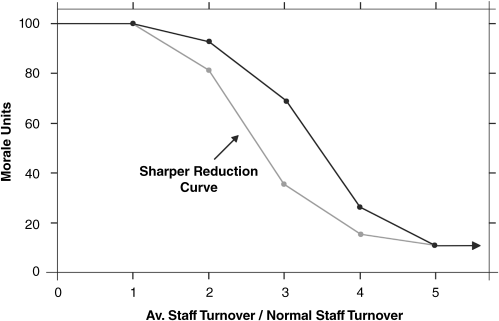
Figure 3.13 Alternative hypothesised X–Y relationships for the effect of staff turnover on team morale.
The range on the Y-axis for the soft variable is typically between 0 and 1.0 or 0 and 100. The full range is shown on the X-axis even though a value of the ratio between 0 and 1.0 will have no effect – it is assumed that an average staff turnover lower than (or equal to) normal staff turnover has no detrimental effect on morale. The range can be extended above 5 if required, but anything beyond two or three times normal staff turnover must be quite serious. The software will linearly interpolate within the line segments as the simulation is on-the-fly and then use the corresponding Y-value for staff morale. The Y-value for the X = 5 point will be used if X > 5.0 and a warning message would be given so the user has the option of extending the curve if necessary. It is assumed that at very high rates of turnover the effect on morale cannot get any worse, so the negative slope tapers off. Also, the general shape of the curve can be experimented with. For instance, a sharper reduction beyond X = 1 or X = 2 might be felt more appropriate (see Figure 3.13), although the overall slope must surely be negative. In general any two line segments in these X–Y relationships should not exhibit a slope reversal (i.e. from negative to positive or vice versa). See Chapter 9 where an instance of an exception to this rule is suggested.
The values used for morale units are arbitrary but the diagram reflects that if morale is really high then 100 can be taken to be a typical value, where a value of, say, 10 or less suggests morale is approaching rock-bottom. It is important to appreciate that, even though the Y-axis units may not be easily confirmed (although an attitude questionnaire might be possible in this case), so long as the X–Y relationship is not changed between policy runs, its effects are captured but in a neutral way. If the relationship is in some sense considered to be ‘wrong’ then that applies equally across all runs. Hence, not only does the comparison between different simulations remain intact, but also, most importantly, a difficult-to-measure but influential variable has been captured.
3.4.2 Co-Flows
There are occasions when it is necessary to model an associated characteristic of a resource in a stock–flow arrangement. For instance, when modelling the physical flow of production in a manufacturing operation, from material processing through to work-in-progress and on to the finished goods stage, it may also be necessary to incorporate the equivalent book value of this sequence of stocks; in other words, we need a separate financial stock–flow arrangement which mirrors the physical flow. This is known as a co-flow arrangement and is the equivalent in SD simulations of the concept of an attribute for an entity often employed in DES. In this case the attribute for the resource involved is value.
The example in Figure 3.14 concerns a totally different application. In a professionally skilled workforce the new employees arrive with a basic level of skill, such as in science-graduate-only recruitment situations, and this is enhanced through, first, in-house training and latterly project experience. One might wish to include not only the numbers at each level of skill, but their collective productivity also. In this example productivity is the attribute concerned. The example shown is intended to represent a software engineering firm where an individual's productivity might be measured in terms of lines of error-free code written per person per month. Departures from the firm are ignored here so as not to clutter the diagram.
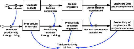
Figure 3.14 Co-flow arrangement for modelling a workforce and their collective productivity.
The co-flow arrangement inevitably involves flouting a normal rule in SD modelling: that is, that direct rate-to-rate connections are not allowed. But it is obvious that as the various physical stocks change, so will the level of the attribute concerned and so a rate-to-rate link is needed. The units for the flows of people in Figure 3.14 are persons/month and the flows representing changes to collective productivity are output/(month ∗ month). This is derived from a multiplication of the person flow (persons/month) by an appropriate individual marginal productivity parameter (output/(persons ∗ month)) which is not shown in the figure.
The co-flow formulation enables an easy assessment of the total productivity (total output capacity) of the entire enterprise. Were it not to be employed it would be necessary to formulate a long auxiliary equation for total productivity which would involve a multiplication and summation of each level of skill's separate contribution to productivity, each based upon its appropriate marginal productivity parameter. However, some may find this more intuitive!
3.4.3 Delays and Smoothing Functions
All dedicated SD software platforms come replete with a library of functions which the modeller can deploy as he or she thinks fit. Among these functions are those for use to represent delays and smoothing and they merit some separate attention in this subsection because they are very frequently used. Because SD separates resource flows and the information flows required to control the resource flows, delay functions are split between resource delays and information delays, although both yield the same effect – a family of exponential delays.
Let us consider resource delays first. Suppose it is desired to model production completion in a manufacturing model or deaths in a population model. In the former case it could be represented as a delayed function of production starts and in the latter as a delayed function of births (ignoring in- and out-migration). Whether a delay function can properly be used is dependent on a crucial criterion. Any delay function implies the use of an internal stock (level) variable which can be made explicit if required. For instance, it would be work-in-progress in the manufacturing example – see Figure 3.15. Where this internal stock ‘drives’ the output then using a delay function is permissible. Work-in-progress cannot be allowed to build up indefinitely and so in a sense is driving the completion of production. In the population example the internal stock is, indeed, population which, by dint of the ageing process which affects any living entity, is driving the death rate. Where the delay output is determined by something elsewhere in the system (other than the internal stock) then a delay function is not indicated.
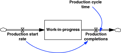
Figure 3.15 Delay construct in the manufacturing example; note rate-to-rate connection and outflow assumed driven by work-in-progress.
Once it has been established that use of a delay function is acceptable, two further determinations need to be made: the value for the average delay time and the order of the delay to be used. In the case of the manufacturing example, the former is the production cycle (or lead) time (Figure 3.15). Its value would be measured in weeks in respect of, say, consumer durables production and months or even years in respect of an aircraft or a naval warship. The determination of the order of the delay function is bound up with the need to understand the transient behaviour of the function (e.g. following a pulse change in the input) and an ability to relate this to the practical situation under consideration.
Consider Figure 3.16 where the transient output from a pulse change in input is presented for three different delay orders – first, third and infinite order (fixed or pipeline delay).
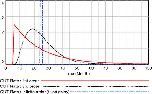
Figure 3.16 Transient output rates from delay functions of various orders (average delay time = 20).
The input PULSE occurs at time t = 5. A first-order delayed response occurs immediately and then progressively declines. The third-order output is initially slower to respond but progressively builds up to a peak and then declines. The fixed delay, as its name implies, merely reproduces the input (not shown) as output, in this case 20 months later. Statistically these are a series of exponential functions which belong to the Erlang family of distributions. The negative exponential response (first-order) is equivalent to an Erlang type 1 distribution. As the order increases, the variance of the distribution of output reduces, so higher orders than 3 would yield narrower and more peaked distributions until ultimately reaching the zero-variance distribution of an infinite-order delay. Clearly, whatever enters the delay function must ultimately leave it, even if this involves a long right-hand tail to the output distribution.
The names for these functions can vary with the software platform chosen. Variants of DELAY1, DELAY3 and DELAY FIXED are employed with an upper case ‘I’ being added at the end of the name where it is required to initialise the delay output to a particular value and this will be included as an additional argument to the function. In the absence of this special case, by default the delay output is initialised to the value of the input. If higher orders than 3 are required then it is permissible to cascade the available functions, but, in general, the three examples offered in Figure 3.16 are the ones most commonly employed.
These functions, which should only ever be used in flow equations, are clearly flexible and can suit different practical circumstances. The first-order function might be used to model deliveries arising from a large order placed for many different items. The third-order version might suit the manufacturing example above, certainly in the case of consumer durables production, whereas the fixed delay might be more appropriate in the case of, say, the construction of a warship.
Turning now to the consideration of information delays, there exists a similar repertoire of functions to those available for resource delays, save for the instance of the infinite delay order. Information delays are used to model the process of decision making. Forrester once famously noted: ‘Management is the process of converting information into action.’ He was distinctly capturing the real-life processes of information collection and assimilation prior to action being taken. These processes are modelled in SD by chains of auxiliary variables which lead into a flow variable. The auxiliaries effectively define action through the control of the flow rates (the policy variables).
Information collection and assimilation processes take time in real life and hence SD models need to reflect these delays. Flow rates are not changed instantaneously, nor can they be observed instantaneously. Sequences of values arising from a flow (and being reported through the formal or informal information systems) may not predicate a trend. Assimilation of this flow of information is necessary in order to reach agreed actionable conclusions.
Information needs to be processed ahead of any action; this is usually referred to as smoothing. The time delay in processing information is commonly referred to as the ‘smoothing time’ or ‘smoothing constant’ and is the second argument in the function following the name of the input variable. First- and third-order smoothing processes are usually available and again have names which can vary with the SD software platform being used: SMOOTH1 and SMOOTH3 are common for first-order and third-order smoothing respectively. The ‘I’ variant is also available should it be required to initialise the output of the smoothing process. By far the most commonly used is first-order smoothing; in fact this is mathematically equivalent to exponential smoothing of the information input stream. Third-order is much less common and tends to be reserved for the more ‘important’ decisions and where there is a discrete delay in the reporting sequence, for example quarterly as opposed to daily or weekly information reports.
Finally, it is worth pointing out that information delays and resource delays possess different properties with respect to mass. A resource delay moves mass from the input to the output variable (i.e. it is conserved) whereas an information source can give up the same information to many different destinations in respect of the policy process – it is non-conserved.
3.4.4 Model Validation
It is probably true to say that SD models are required to undergo much higher standards of validation than other methodologies and techniques associated with the fields of management science and econometrics. It is a commendation for the SD research community that it has responded and there now exists a significant range of tests which can be used to validate an SD model. It must be emphasised from the outset, however, that no model can be shown to represent the ultimate truth and a primary objective of the process of subjecting a model to various tests is to enhance its suitability for use in policy analysis. Where the work is for clients, it is necessary for them to be sufficiently confident of the internal mechanics and robustness of the model and then to go on and put into action the policy advice which might emerge from the simulation runs. Validation tests can be seen, therefore, as enhancing confidence in the model – nothing more and nothing less.
It is not the intention here to go into great detail of the range of tests now available for SD models. Various references can be consulted. An early, oft-cited contribution is that of Forrester and Senge (1980). Sterman (2000) offers considerable detail on the matter, some material being derived from his earlier article describing appropriate metrics for the historical fit of simulated to reported data (Sterman, 1984). Coyle and Exelby (2000) give attention explicitly to the validation of commercial SD models, while Barlas has a number of publications in this domain, a notable one being Barlas (1996). Finally, Schwaninger and Grösser (2009) offer a contemporary overview of SD model validation.
Model verification is a necessary step in DES modelling. It is the task of demonstrating that the coded model is the one intended by the modeller. This is different to model validation, which is more concerned with an external assessment and how well the model corroborates with the real-world system it purports to represent. In respect of SD modelling, a dimensional analysis check (see Section 3.3.4) could be construed as a verification task, but there also exists a test which accords with model verification and which does not always appear in the list of SD model tests published elsewhere: this is the mass-balance check.
It is obvious that, in a model where flows of resources are represented, the amount flowing in must balance with the amount flowing out. In other words, the model must not gain or lose mass. The need for this check is enhanced when the resource flows in the model involve multiple inflows and bifurcations, although there is no harm carrying out the check even with a simple one-way flow system.
It is necessary to cumulate all the inflows and outflows for each resource being modelled. Then, taking account of both initial values and the values of the various stocks at any one time, the balance (or checksum) equation has the form
Given the inevitably large numbers which will be involved either side of the minus sign, it is necessary to deploy a double precision version of the software being used. The correct result should be computationally equivalent to zero throughout the run; anything else indicates a flawed model. Where more than one resource flow is involved (e.g. people and finance) then separate checksum equations need to be used – one for each flow.
To conclude this subsection it is worthwhile to align important validation tests against the three main categories of SD model. These categories are: (A) a model representing an existing real-world system where there is knowledge extant for that system and an issue which needs addressing (models built for consultancy assignments, and where a client exists, usually fall into this category); (B) a model of a generic system, addressing a specific issue but not parameterised to any particular real-world system (models developed in academic research are often examples of this type); (C) a model of a system that does not yet exist but where there is a need to anticipate matters which might affect the design of that system (the setting for this type could be either consulting or academic research).
With models of type A there will be an emphasis on behaviour reproduction tests. It is necessary to demonstrate a correspondence between the simulated output and reported data. This correspondence need only be qualitative; point-for-point equivalence is neither sought nor is necessary. Goodness-of-fit metrics can, however, be calculated. The use of R2 is common but a more appropriate metric is Theil's inequality statistics. This decomposes the mean square error into three components and then determines the fraction of the error due to each. Sterman (2000, p. 876) outlines different possible outcomes and the interpretation of the statistic. Given knowledge of the system being modelled, the model's face validity and its constituent parameter values can also be subject to collective scrutiny by the clients as a further validation check in this case.
In the case of models of type B the output behaviour needs to be plausible. That is to say, important constituent variables should not produce behaviour which is ‘obviously wrong’. Generally, a reference mode behaviour will be known. This is a sketch graph of the typical dynamic behaviour of this type of system; the model needs to conform qualitatively to this behaviour. In addition it may be possible to assemble a range of experts with an intimate knowledge of such systems and utilise their collective expertise to assess the model's face validity.
Finally, in the case of models of type C, behaviour reproduction tests are clearly impossible and the emphasis will fall solely onto the model's face validity. The formation of an expert group is almost mandatory here and, as far as possible, unanimity among the members as to the model's structure and behaviour is sought.
3.4.5 Optimisation of SD Models
The term ‘optimisation’ when related to SD models has a special significance. It relates to the mechanism used to improve the model vis-à-vis a criterion. This collapses into two fundamentally different intentions. First, one may wish to improve the model in terms of its performance. For instance, it may be desired to minimise the overall costs of inventory while still offering a satisfactory level of service to the downstream customer. So the criterion here is cost and this would be minimised after searching the parameter space related to service level. The direction of need may be reversed and maximisation may be desired as if, for instance, one had a model of a firm and wished to maximise profit subject to an acceptable level of payroll and advertising costs. Here the parameter space being explored would involve both payroll and advertising parameters. This type of optimisation might be described generically as policy optimisation.
A separate improvement to the model may be sought where it is required to fit the model to past time series data. Optimisation here involves minimising a statistical function which expresses how well the model fits a time series of data pertaining to an important model variable. In other words, a vector of parameters is explored with a view to determining the particular parameter combination which offers the best fit between the chosen important model variable and a past time series dataset of this variable. This type of optimisation might be generically termed model calibration. If all the parameters in the SD model are determined in this fashion then the process is equivalent to the technique of econometric modelling. A good comparison between SD and econometric modelling can be found in Meadows and Robinson (1985).
In respect of calibration optimisation, there is also the possibility of fitting the model to projected future behaviour. If a future target is set in terms of some performance metric, then to associate that with a particular trajectory for its attainment is a significant improvement on just determining a target as a single point x time periods ahead. Not least, this approach helps to verify if the chosen target is actually feasible. Model optimisation in this mode can be seen as a synthesis of policy optimisation and calibration optimisation.
The process by which an SD model is optimised involves pre-selecting the parameters to be included in the search vector, associating each parameter with a range in which the search will be conducted and finally determining the objective function to be optimised. The software will repeatedly simulate, for thousands of runs if required, searching for the values of the particular parameter combination which will conform with the maximum or minimum value of the objective function, as appropriate.
More details on the mechanisms of SD model optimisation can be found in Keloharju and Wolstenholme (1988), Dangerfield and Roberts (1996) and Dangerfield (2009). Examples are reported in Keloharju and Wolstenholme (1989), Dangerfield and Roberts (1999), Graham and Ariza (2003) and also in Dangerfield (2009).
3.4.6 The Role of Data in SD Models
In many cases where the author has suggested an SD approach to a policy issue the rejoinder has been: ‘What data will you require to accomplish this?’ There is an implicit assumption by lay people that ‘modelling’ must involve enormous quantities of data and this puts a brake on its possible use. In fact in the case of SD simulation models the answer to the amount of data required in order to produce a working model is: ‘Surprisingly little’.
It is a fact, though, that the amount of data required for a modelling exercise varies significantly with the technique being adopted. Confining the discussion to the domain which might be loosely termed ‘dynamic systems models’, on one extreme lies econometric modelling where every variable requires sufficient historical time series data in order to fit the model. If no historical data exists for an important variable then sometimes a proxy can be formulated from the data which does exist, but, failing this, the variable has to be excluded from the model. Further, there is no provision in econometrics for the incorporation of soft variables as discussed above in Section 3.4.1.
The amount of data required for a DES model lies somewhere on the continuum between econometrics and SD. All activity durations need to be estimated, usually by fitting a theoretical probability distribution to reported data. Further, a maximum number may need to be established for certain entities (e.g. beds on a hospital ward) along with any limits on queue sizes.
In the case of SD the extent of required data can be framed in the knowledge that such models can be created for systems which do not yet exist (i.e. operating in a design mode). Here the data required is simply parameter values, such as productivity of the workforce (output units/person/time unit), delay in adjusting capital stock (time unit), fat quantity in meals outside (grams/meal) or probability of default on debt (dimensionless) together with estimates for the initial values of each of the stocks (levels) in the model. All of these numerical quantities would then be guesstimated by the modeller with the help of the clients if available.
Should the system being studied already exist then statistical estimates or generally accepted and reliable knowledge can replace the guesstimates of parameter values for the SD model. Further, if working on a specific policy issue, past time series data may be available for certain model variables and this data can be embraced as part of the process of model validation (see Section 3.4.4). Therefore, in respect of SD models, the maxim on requisite data is: nothing is required, but if any data exists then by all means use it.
3.5 Further Reading
It is impossible in this single chapter to do full justice to what is now a significant methodology in the socio-economic, managerial, health, biological, environmental, energy and military sciences. However, three contemporary books will take the interested reader much further. These are purely the author's choice and they are listed in order of page count.
John Sterman's book (982pp.) has arguably the most comprehensive coverage; see Sterman (2000) in the reference list. John Morecroft's (466pp.) Strategic Modelling and Business Dynamics: A feedback systems approach (2007), published by John Wiley & Sons, Ltd, Chichester, offers a very wide coverage of systems thinking and SD and incorporates many practical model examples. Third, Kambiz Maani and Bob Cavana have written a second edition of their offering (288pp.): K.E. Maani and R.Y. Cavana (2007) Systems Thinking, System Dynamics: Managing change and complexity, published by Pearson Education NZ (Prentice Hall), Auckland.
All these books come with a CD-ROM and/or a web site which provides specimen models to be run and allows scenario experiments to be conducted. Exercises and instructor's manuals are also available.
Notes
References
- Ballé, M. (1994) Managing with Systems Thinking, McGraw-Hill, London.
- Barlas, Y. (1996) Formal aspects of model validity and validation in system dynamics. System Dynamics Review, 12 (3), 183–210.
- Coyle, G. and Exelby, D. (2000) The validation of commercial system dynamics models. System Dynamics Review, 16 (1), 27–41.
- Coyle, R.G. (2000) Qualitative and quantitative modelling in system dynamics: some research questions. System Dynamics Review, 16 (3), 225–244.
- Coyle, R.G. (2001) Rejoinder to Homer and Oliva. System Dynamics Review, 17 (4), 357–363.
- Dangerfield, B.C. (2009) Optimization of system dynamics models, in Encyclopedia of Complexity and Systems Science (ed. R.A. Meyers), Springer, New York, pp. 9034–9043. (Reprinted in Complex Systems in Finance and Econometrics, Springer, New York, 2011, 802–811.)
- Dangerfield, B.C. and Roberts, C.A. (1996) An overview of strategy and tactics in system dynamics optimisation. Journal of the Operational Research Society, 47 (3), 405–423.
- Dangerfield, B.C. and Roberts, C.A. (1999) Optimisation as a statistical estimation tool: an example in estimating the AIDS treatment-free incubation period distribution. System Dynamics Review, 15 (3), 273–291.
- Forrester, J.W. (1958) Industrial dynamics – a major breakthrough for decision makers. Harvard Business Review, 36 (4), 37–66.
- Forrester, J.W. (1961) Industrial Dynamics, MIT Press, Cambridge, MA (now available from the System Dynamics Society, Albany, NY).
- Forrester, J.W. (2007) System dynamics – a personal view of the first fifty years. System Dynamics Review, 23 (2–3), 345–358.
- Forrester, J.W. and Senge, P.M. (1980) Tests for building confidence in system dynamics models, in System Dynamics (eds A.A. Legasto Jr, J.W. Forrester and J.M. Lyneis), North-Holland, Amsterdam, pp. 209–228.
- Goodman, M.R. (1974) Study Notes in System Dynamics, Wright-Allen Press, Cambridge, MA (now available from the System Dynamics Society, Albany, NY).
- Graham, A.K. and Ariza, C.A. (2003) Dynamic, hard and strategic questions: using optimisation to answer a marketing resource allocation question. System Dynamics Review, 19 (1), 27–46.
- Hardin, G. (1968) The tragedy of the commons. Science, 162 (3859), 1243–1248. doi: 10.1126/science.162.3859.1243
- Homer, J. and Oliva, R. (2001) Maps and models in system dynamics: a response to Coyle. System Dynamics Review, 17 (4), 347–355.
- Keloharju, R. and Wolstenholme, E.F. (1988) The basic concepts of system dynamics optimisation. Systems Practice, 1, 65–86.
- Keloharju, R. and Wolstenholme, E.F. (1989) A case study in system dynamics optimisation. Journal of the Operational Research Society, 40 (3), 221–230.
- Maruyama, M. (1963) The second cybernetics: deviation-amplifying mutual causal processes. American Scientist, 51 (2), 164–179.
- Meadows, D.L. and Sterman, J. (2012) Fishbanks: A Renewable Resource Management Simulation, https://mitsloan.mit.edu/LearningEdge/simulations/fishbanks/Pages/fish-banks.aspx (accessed 30 May 2013).
- Meadows, D.M. and Robinson, J.M. (1985) The Electronic Oracle, John Wiley & Sons, Ltd, Chichester (now available from the System Dynamics Society, Albany, NY).
- Merrill, J.A., Deegan, M., Wilson, R.V. et al. (2013) A system dynamics evaluation model: implementation of health information exchange for public health reporting. Journal of the American Medical Informatics Association, 20, e131–e138. doi: 10.1136/amiajnl-2012-001289
- Richardson, G.P. (2011) Reflections on the foundations of system dynamics. System Dynamics Review, 27 (3), 219–243.
- Richardson, G.P. and Pugh, A.L. (1981) Introduction to System Dynamics Modelling with DYNAMO, MIT Press, Cambridge, MA (now available from the System Dynamics Society, Albany, NY).
- Schwaninger, M. and Grösser, S. (2009) System dynamics modelling: validation for quality assurance, in Encyclopedia of Complexity and Systems Science (ed. R.A. Meyers), Springer, New York, pp. 9000–9014. (Reprinted in Complex Systems in Finance and Econometrics, Springer, New York, 2011, 767–781.)
- Senge, P. (1990) The Fifth Discipline, Currency Doubleday, New York.
- Senge, P., Kleiner, A., Roberts, C. et al. (1994) The Fifth Discipline Fieldbook, Currency Doubleday, New York.
- Sherwood, D. (2002) Seeing the Forest for the Trees: A Manager's Guide to Applying Systems Thinking, Nicholas Brealey, London.
- Sterman, J.D. (1984) Appropriate summary statistics for evaluating the historical fit of system dynamics models. Dynamica, 10 (2), 51–66.
- Sterman, J.D. (2000) Business Dynamics: Systems Thinking and Modeling for a Complex World, Irwin McGraw-Hill, New York.
- Tustin, A. (1953) The Mechanism of Economic Systems, Harvard University Press, Cambridge, MA.
- Wolstenholme, E.F. (2003) Towards the definition and use of a core set of archetypal structures in system dynamics. System Dynamics Review, 19 (1), 7–26.