
8
An Empirical Study Comparing Model Development in Discrete-Event Simulation and System Dynamics*
Antuela Tako and Stewart Robinson
School of Business and Economics, Loughborough University, UK
8.1 Introduction
Simulation is a modelling tool widely used in operational research (OR), where computer models are deployed to understand and experiment with a system (Pidd, 2004). Two of the most established simulation approaches are discrete-event simulation (DES) and system dynamics (SD). They both started and evolved almost simultaneously with the advent of computers (Wolstenholme, 1990; Robinson, 2005), but very little communication existed between these fields (Lane, 2000; Brailsford and Hilton, 2001). This is, however, changing with more DES and SD academics and practitioners showing an interest in the other's world (Morecroft and Robinson, 2005). Unfortunately there is little assistance for this interest, since work reporting on comparisons of the two simulation approaches is limited. The comparisons that exist are mostly opinion based, derived from the authors' personal views based on their field of expertise. Hence, little understanding exists regarding the differences and similarities between the two simulation approaches. More specifically, this chapter explores the model development process as followed by expert modellers in each field.
Both DES and SD models are simplified representations of a system developed with a view to understanding its performance over time and to identifying potential means of improvement. DES represents individual entities that move through a series of queues and activities at discrete points in time. Models are generally stochastic in nature. DES has been traditionally used in the manufacturing sector, while recently it has been increasingly used in the service sector (Robinson, 2005). Some key DES applications include airports, call centres, fast food restaurants, banks, health care and business processes.
In SD, systems are modelled as a set of stocks and flows, adjusted in pseudo-continuous time. SD models are based on differential equations and are generally deterministic. Feedback, which results from the relationships between the variables in the model, is an important feature in SD models. SD has been applied to a wide range of problems. Applications include economic behaviour, politics, psychology, defence, criminal justice, energy and environmental problems, supply chain management, biological and health care modelling, project management, educational problems, staff recruitment and also manufacturing (Wolstenholme, 1990).
While the underlying aims of using the two simulation approaches are similar, it is our belief that the approach to modelling is very different among the two groups of modellers. This chapter provides an empirical study that compares the model development process followed in each respective field. The study follows the processes used by 10 expert modellers, five from each field, during a simulation modelling task. Each expert was asked to build a simulation model from a case study on forecasting the UK prison population. The case was specifically designed to be suitable for both DES and SD. Verbal protocol analysis (Ericsson and Simon, 1984) was then used to identify the processes that the modellers followed. This study provides a quantitative analysis that compares the modelling process followed by the DES and SD modellers. Its key contribution is to provide empirical evidence on the comparison of the DES and SD model development process. Its underlying aim is to bring closer the two fields of simulation, with a view to creating a common basis of understanding.
The chapter is outlined as follows. It starts with a review of the existing literature comparing DES and SD, including the comparison of the model development process in DES and SD modelling as described in the literature. This is then followed by an explanation of the research approach, describing the case study, the participants, verbal protocol analysis and the coding undertaken. The results of the study, including the quantitative analysis of the protocols of the 10 expert modellers and some observations on how they tackle the case, are then presented. Finally, the main findings and the limitations of the study are discussed.
8.2 Existing Work Comparing DES and SD Modelling
This section reviews the existing literature on the comparison of the two simulation approaches, DES and SD. First, the main comparison studies are briefly considered in chronological order, followed by an account of the views expressed on the model development process in DES and SD.
The first comparison work was that of Meadows (1980) which looked into the epistemological stance taken in SD as a modelling approach and in econometrics (representative of DES). Based on the basic characteristics and the limitations of each paradigm, the author goes on to identify a paradigm conflict resulting from the modellers' perception of the world and the problems concerned, the procedures they use to go about solving them, as well as the validity of model outcomes.
Coyle (1985) approaches the discussion from a SD perspective, while considering ways to model discrete events in an SD environment. His comparison focuses on two aspects: randomness existing in DES modelling and model structure; he claims that open- and closed-loop system representations are developed in DES and SD respectively.
In her doctoral thesis, Mak (1993) developed a prototype of automated conversion software, where she investigates the conversion of DES activity cycle diagrams into SD stock and flow diagrams. DES process flow diagrams, which could be considered as more close to stock and flow diagrams, were not considered in her study.
Baines et al. (1998) provide an experimental study of various modelling techniques, on DES and SD among others, and their ability to evaluate manufacturing strategies. The authors comment on the capability of a modelling technique based on the time taken in building models, flexibility, model credibility and accuracy.
Sweetser (1999) compares DES and SD based on the established modelling practice and the conceptual views of modellers in each area. He maintains that both simulation approaches can be used to understand the way systems behave over time and to compare their performance under different conditions. When comparing the two simulation approaches, Sweetser considers the following aspects: feedback effects and system performance, mental models, systems' view and type of systems represented, the model building process followed and finally validation of DES and SD models. Two DES and SD conceptual models of an imaginary production line are then compared.
Brailsford and Hilton (2001) compare DES and SD in the context of health care modelling. The authors compare the main characteristics and the application of the two approaches, based on two specific health care studies (SD and DES) and on their own experience as modellers. At the end, they provide a list of criteria to assist in the choice between the two simulation approaches, considering problem type, model purpose and client requirements. Theirs is only a tentative list and they admit that the decision is not simple and straightforward.
Lane (2000) provides a comparison of DES and SD, focusing mainly on the conceptual differences. Considering three modes of discourse, Lane maintains that DES and SD can be presented as different or similar based on the position taken (the mode of discourse). In the third discourse a mutual approach is taken. The main comparison aspects considered are: the modeller's perspective on complexity, data sources, problem type, model elements, human agents, model validity and outputs. It should be noted that some of the statements have been contradicted. For example, model outputs in DES do not always represent point predictions (Morecroft and Robinson, 2005). An example of a DES model used to understand the system behaviour can be found in the paper by Robinson (2001).
Morecroft and Robinson (2005) is the first study that undertakes an empirical comparison, using a fishery model. The authors build a step-by-step simulation model, using DES (Robinson) and SD (Morecroft) modelling. However, one could claim the existence of bias, as the two modellers were aware of each other's views on modelling. The authors conclude with a list of differences between DES and SD, regarding system representation and interpretation. They become aware of the different modelling philosophies they take when developing their models, but they still contemplate that there is not a straightforward distinction between the two approaches, but rather it is a result of careful consideration of various criteria.
An empirical study on the comparison of DES and SD from the users' point of view has been carried out by Tako and Robinson (2009). The authors found that users' perceptions of two simple DES and SD models were not significantly different, implying that from the user's point of view the type of simulation approach used makes little difference if any, as long as it is suitable for addressing the problem situation at hand. So far, no study has been identified that provides an unbiased empirical account on the comparison of the DES and SD model development process.
The opinions expressed regarding the comparison of DES and SD are built around three main areas: the practice of model development; modelling philosophy; and the use of respective models. There appears to be a general level of agreement in the opinions stated on the nature of the differences, but also exceptions and contradictions exist. In addition, limited empirical work has been done to support the statements found in the literature. A long list of the views expressed can be compiled. Table 8.1 provides only some of the key differences proposed in the literature.
Table 8.1 Examples of views expressed on the comparison of DES and SD modelling.
| Aspects compared | DES | SD | Author(s) |
| Nature of problems modelled | Tactical/operational | Strategic | Sweetser, 1999; Lane, 2000 |
| Feedback effects | Models open-loop structures – less interested in feedback | Models closed-loop structures based on causal relationships and feedback effects | Coyle, 1985; Sweetser, 1999; Brailsford and Hilton, 2001 |
| System representation | Analytic view | Holistic view | Baines et al., 1998; Lane, 2000 |
| Complexity | Narrow focus with great complexity and detail | Wider focus, general and abstract systems | Lane, 2000 |
| Data inputs | Quantitative, based on concrete processes | Quantitative and qualitative, use of anecdotal data | Sweetser, 1999; Brailsford and Hilton, 2001 |
| Validation | Black-box approach | White-box approach | Lane, 2000 |
| Model results | Provides statistically valid estimates of system performance | Provides a full picture (qualitative and quantitative) of system performance | Meadows, 1980; Mak, 1993 |
8.2.1 DES and SD Model Development Process
Considering the modelling process, as suggested in DES and SD textbooks teaching the art of modelling, one can identify similarities between the two approaches, especially in terms of the stages involved. It is clear that the main stages followed are equivalent to generic OR modelling (Hillier and Lieberman, 1990; Oral and Kettani, 1993; Willemain, 1995), which include: problem definition; conceptual modelling; model coding; model validity; model results and experimentation; implementation. For instance, see Figure 8.1 which shows a typical DES modelling process from Robinson (2004).
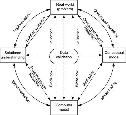
Figure 8.1 The DES modelling process based on (Robinson, 2004, p. 211). Reproduced with permission from the McGraw-Hill Companies.
The main aspects pertaining to the model development process are considered next. First, it is claimed that during the DES model building process emphasis is put on the development of the model on the computer (model coding). In their experimental study, Baines et al. (1998) commented specifically that the time taken in building a DES model was considerably longer compared with a SD model. Furthermore, Artamonov (2002) developed two equivalent DES and SD models of the beer distribution game model (Senge, 1990) and commented on the difficulty involved in coding the model on the computer. He found the development of the model on the computer more difficult in the case of the DES approach, whereas the development of the SD model was less troublesome. Baines et al. (1998) attributes this to the fact that DES encourages the construction of a more lifelike representation of the real system compared with other techniques, hence resulting in a more detailed and complex model.
On the other hand, Meadows (1980) highlights that system dynamicists spend most of their modelling time specifying the model structure. Specification of the model structure consists of the representation of the causal relationships that generate the dynamic behaviour of the system. This is equivalent to the development of the conceptual model.
Another feature concerning DES and SD model development is the iterative nature of the modelling process. In DES and SD textbooks, it is highlighted that simulation modelling involves a number of repetitions and iterations (Randers, 1980; Sterman, 2000; Pidd, 2004; Robinson, 2004). Indeed, an iterative modelling process is depicted in Figure 8.1 for both DES and SD. Regardless of the modeller's experience, a number of repetitions occur from the creation of the first model, until a better understanding of the real-life system is achieved. So long as the number of iterations remains reasonable, these are in fact quite desirable (Randers, 1980).
8.2.2 Summary
The existing studies comparing DES and SD tackle three main areas of modelling: the practice of model development; modelling philosophy; and the use of models. These studies, however, are mostly opinion based and lack any empirical basis. We focus on the model development process in each field (DES and SD). The key aspects identified consist of the amount of attention paid to the different stages during modelling, the sequence of modelling stages followed, and the pattern of iterations followed. Taking an empirical perspective, we examine in this chapter the statements found in the literature by following the model development process adopted by expert DES and SD modellers. While it is expected that DES and SD modellers pay different levels of attention to different modelling stages, both DES and SD modellers are expected to follow iterative modelling processes. However, we do not have specific expectations about the exact pattern of iteration that the two groups of modellers will follow.
8.3 The Study
The overall objective of the study is to compare empirically the stages followed by expert modellers while undertaking a simulation modelling task. We believe that DES and SD modellers think differently during the model development process. Therefore, it is expected that while observing DES and SD experts developing simulation models, these differences become evident. The authors use qualitative textual analysis (Miles and Huberman, 1994) and perform a quantitative analysis of the resulting data to identify the differences and similarities in the model development process. The current chapter compares DES and SD modellers' thinking process by analysing the modelling stages they think about while developing simulation models. The aim is to compare the model building process followed by DES and SD modellers regarding: the attention paid to different modelling stages, the sequence of modelling stages followed, and the pattern of iterations. In order to provide a more complete picture, some observations are also made on the models developed and the DES and SD experts' reactions during the modelling sessions.
This section explains the study undertaken. First, the case study used is briefly described, followed by a brief introduction to the research method employed, namely verbal protocol analysis (VPA). Next, we report on the profile of the participants involved in the study and the coding process carried out.
8.3.1 The Case Study
A suitable case study for this research needs to be sufficiently simple to enable the development of a model in a short period of time (60–90 minutes). In addition it needs to accommodate the development of models using both simulation techniques so that the specific features of each technique (randomness in DES vs deterministic models in SD, aggregated presentation of entities in SD vs individual representation of entities in DES, etc.) are present.
After considering a number of possible contexts, the prison population problem was selected. The prison population case study, where prisoners enter prison initially as first-time offenders and are then released or return to prison as recidivists, can be represented by simple simulation models using both DES and SD. Both approaches have been previously used for modelling the prison population system. DES models of the prison population have been developed by Kwak, Kuzdrall and Schniederjans (1984), Cox, Harrison and Dightman (1978) and Korporaal et al. (2000), while SD models have been developed by Bard (1978) and McKelvie et al. (2007); the UK prison population model of Grove, MacLeod and Godfrey (1998) is a flow model analogous to an SD model.
The UK prison population example used in this research is based on Grove, MacLeod and Godfrey (1998). The case study starts with a brief introduction to the prison population problem with particular attention to the issue of overcrowded prisons. Descriptions of the reasons for and impacts of the problem are provided. More specifically, two types of offenders are considered, petty and serious. There are in total 76 000 prisoners in the system, of which 50 000 are petty and 26 000 serious offenders. Offenders enter the system as first-time offenders and receive a sentence depending on the type of offence; on average 3000 petty offenders vs 650 serious offenders enter each year. Petty offenders receive a shorter sentence (on average 5 years vs 20 years for serious offenders). After serving time in prison they are released. A proportion of the released prisoners reoffend and go back to gaol (recidivists) after two years (on average), whereas the rest are rehabilitated. The figures and facts used in the case study are mostly based on reality, but slightly adapted for the purposes of the research. The modellers were provided with a basic conceptual model (Figure 8.2) and some initial data (i.e. the initial number of petty and serious offenders), while other data, namely statistical distributions, were intentionally omitted in order to observe modellers' reactions. The task for participating modellers was to develop a simulation model to be used as a decision-making tool by policy makers. For more details of the case study the reader is referred to Tako and Robinson (2009).

Figure 8.2 A simple diagram depicting a conceptual model of the UK prison population case study.
8.3.2 Verbal Protocol Analysis
VPA is a research method derived from psychology. It requires the subjects to ‘think aloud’ when making decisions or judgements during a problem-solving exercise. It relies on the participants' generated verbal protocols in order to understand in detail the mechanisms and the internal structure of cognitive processes that take place (Ericsson and Simon, 1984). Therefore, VPA as a process tracing method provides access to the activities that occur between the onset of a stimulus (case study) and the eventual response to it (model building) (Ericsson and Simon, 1984; Todd and Benbasat, 1987). Willemain (1994, 1995) was the first to use VPA in OR to document the thought processes of OR experts while building models.
VPA is considered to be an effective method for the comparison of the DES and SD model building process. It is useful because of the richness of information and the live accounts it provides on the experts' modelling process. Another potential research method would have been to observe real-life simulation projects, using DES and SD. This would, however, mean that only two situations could be used, which would result in a very small sample size. Additionally, for a valid comparison it is necessary to have comparable modelling situations, which would require two potential real-life modelling projects of equivalent problem situations. The potential for getting access to two modelling projects of a similar situation was deemed unfeasible. We also considered running interviews with modellers from the DES and SD fields. Given that the overall aim of this research is to go beyond opinions and to get an empirical view about model development, one can claim that modellers' reflections may not reflect correctly the processes followed during model building and this would therefore not represent a full picture of model building. Hence, interviews were not considered appropriate. VPA on the other hand mitigates the issues related to the aforementioned research methods, as it can capture modellers' thoughts in practical modelling sessions in a controlled experimental environment, using a common stimulus – the case study.
Protocol analysis as a technique has its own limitations. The verbal reports may omit important data (Willemain, 1995) because the experts, being under observation, may not behave as they would normally. The modellers are asked to work alone and this way of modelling may not reflect their usual practice of model building, where they would interact with the client, colleagues, and so on. In addition, there is a risk that participants do not ‘verbalise’ their actual thoughts, but are only ‘explaining’. To overcome this and to ensure that the experts speak their thoughts aloud, short verbalisation exercises, based on Ericsson and Simon (1984), were run at the beginning of each session.
8.3.3 The VPA Sessions
The subjects involved in this study were provided with the prison population case study at the start of the VPA session and were asked to build simulation models using their preferred simulation approach. During the modelling process the experts were asked to ‘think aloud’ as they model. The researcher (Tako) sat in the same room, but social interaction with the subjects was limited. She only intervened in the case when participants stopped talking for more than 20 seconds to tell them to ‘keep talking’. The researcher was also answering explanatory questions, providing participants with additional data inputs (if they asked for them) and prompting them to build a model on the computer in the case when they did not do so under their own initiative. The modelling sessions were held in an office environment with each individual participant. The sessions lasted approximately 60–90 minutes. The participants had access to writing paper and a computer with relevant simulation software (e.g. SIMUL8, Vensim, Witness, Powersim, etc.). The expert modellers chose to use the software they used as part of their work and hence were more familiar with. The protocols were recorded on audio tape and then transcribed.
8.3.4 The Subjects
The subjects involved in the modelling sessions were 10 simulation experts in DES and SD modelling, five in each area. The sample size of 10 participants is considered reasonable, although a larger sample would, of course, be better. According to Todd and Benbasat (1987), due to the richness of data found in one protocol, VPA samples tend to be small, between 2 and 20.
For reasons of confidentiality participants' names are not revealed. In order to distinguish each participant we use the symbol DES or SD, according to the simulation technique used, followed by a number. So DES modellers are called DES1, DES2, DES3, DES4 and DES5, while SD subjects are SD1, SD2, SD3, SD4 and SD5. All participants use simulation modelling (DES and SD) as part of their work, most of them holding consultant posts in different organisations. The companies they come from are established simulation software companies or consultancy companies based in the UK.
A mixture of backgrounds within each participant group (DES and SD) was sought. All participants have completed either doctorates or masters' degrees in engineering, computer science, OR or hold MBAs. Their experience in modelling ranges from at least 6 years up to 19 years. They have also acquired supplementary simulation training as part of their jobs. They boast an extensive experience of modelling in areas such as the National Health Service, criminal justice, the food and drinks sector, supply chains, and so on. A list of the expert modellers' experience and the software used in the modelling sessions is provided in Table 8.2.
Table 8.2 List of DES and SD modellers' profiles.
| DES modeller | Modelling experience | DES software used | SD modeller | Modelling experience | SD software used |
| DES1 | 9 years | Witness | SD1 | 14 years | Stella/iThink |
| DES2 | 4 years | SIMUL8 | SD2 | 16 years | Strategy dynamics |
| DES3 | 13 years | Flexim | SD3 | 5 years | Powersim |
| DES4 | 8 years | SIMUL8 | SD4 | 20 years | Stella/iThink |
| DES5 | 4 years | Witness | SD5 | 8 years | Vensim |
8.3.5 The Coding Process
A coding scheme was designed in order to identify what the modellers were thinking about in the context of simulation model building. The coding scheme was devised following the stages of typical DES and SD simulation projects, as in Robinson (2004), Law (2007), Sterman (2000) and Randers (1980). Each modelling topic has been defined in the form of questions corresponding to the modelling stage considered. The modelling topics and their definitions are as follows:
- Problem structuring: What is the problem? What are the objectives of the simulation task?
- Conceptual modelling: Is a conceptual diagram drawn? What are the parts of the model? What should be included in the model? How to represent people? What variables are defined?
- Model coding: What is the modeller entering on the screen? How is the initial condition of the system modelled? What units (time or measuring) are used? Does the modeller refer to documentation? How to model the user interface?
- Data inputs: Do modellers refer to data inputs? How are the already provided data used? Are modellers interested in randomness? How are missing data derived?
- Verification and validation: Is the model working as intended? Are the results correct? How is the model tested? Why is the model not working?
- Model results and experimentation: What are the results of the model? What sort of results is the modeller interested in? What scenarios are run?
- Implementation: How will the findings be used? What learning is achieved?
The coding process starts with the definition of a coding scheme. Initially, the recordings of each verbal protocol were transcribed and then divided into episodes or ‘thought’ fragments, where each fragment is the smallest unit of data meaningful to the research context. Each single episode was then coded into one of the seven modelling topics or an ‘other’ category for verbalisations that were not related to the modelling task. Some episodes, however, referred simultaneously to two modelling topics and were, therefore, coded as containing two modelling topics.
Regarding the nature of the coding process followed, a mix of top-down and bottom-up approaches to coding was taken (Ericsson and Simon, 1984; Patrick and James, 2004). A theoretical base was already established (the initially defined modelling topics), which enabled a top-down approach. Throughout the various checks of the coded protocols undertaken, the coding categories were further redefined through a bottom-up approach. An iterative coding process was followed, where the coding scheme was refined and reconsidered as more protocols were coded. Pilot studies were initially carried out to test the case study, use of VPA and the coding scheme. The coding scheme was refined during the pilots and to some extent during the coding of the 10 protocols.
The transcripts were coded manually using a standard word processor. According to Willemain (1995), the coding process requires attention to the context a phrase is used in and, therefore, subjectivity in the interpretation of the scripts is unavoidable. In order to deal with subjectivity, multiple independent codings were undertaken in two phases. In the first stage, one of the researchers (Tako) coded the transcripts twice with a gap of three months between coding. Overall, a 93% agreement between the two sets of coding was achieved, which was considered acceptable. The differences were examined and a combined coding was reached. Next, the coded transcripts with the combined codes were further blind-checked by a third party, knowledgeable in OR modelling and simulation. In the cases where the coding did not agree, the researcher who undertook the coding and the third party discussed the differences and re-examined the episodes to arrive at a consensus coding. Overall, a 90% agreement between the two codings was achieved, which was considered satisfactory compared with the minimum 80% match value suggested as acceptable by Chi (1997). A final examination of the coded transcripts was undertaken to check the consistency of the coded episodes. Some more changes were made to the definition of modelling topics, but these were fairly minor. The results from the coded protocols are now presented and discussed.
8.4 Study Results
This section presents the results of a quantitative analysis of the 10 coded protocols. The data represent a quantitative description of participants' modelling behaviour, exploring the distribution of attention to modelling topics, the sequence of modelling stages during the model building exercise and the pattern of iterations followed among topics. The findings from each analysis follow.
8.4.1 Attention Paid to Modelling Topics
In order to explore the distribution of attention by modelling topic, the number of words articulated is used as a measure of the amount of verbalisations made by the expert modellers. In turn, this is used to indicate the spread of modellers' attention to the different modelling topics. While Willemain used lines as a measure of verbalisation in his study of modellers' behaviour (Willemain, 1995; Willemain and Powell, 2006), we believe that word counts are a more accurate measure, since they avoid the misrepresentation caused by counting incomplete (half or three-quarter) lines as full lines. This is particularly relevant when measuring the amount of verbalisation in each episode, where the protocol is divided into smaller units, including more incomplete lines. The average number of words articulated in the DES and SD protocols by modelling topic is compared in order to establish significant differences between the two groups. Figure 8.3 shows the number of words verbalised by modelling topic by the two groups of modellers. The corresponding numerical values for the average number of words and the standard deviation for the two groups of modellers are also provided against each modelling topic. Comparing the total number of words verbalised in the overall DES and SD protocols, an average difference of 1751 words is identified, suggesting that DES modellers verbalise more than SD modellers. The equivalent box plots of the total number of words verbalised by DES and SD modellers in Figure 8.3 (bottom) show that, while the medians are similar, there is a bigger variation in the total number of words verbalised by DES modellers.
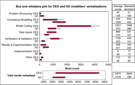
Figure 8.3 Box and whiskers plot of DES and SD modellers' verbalisations by modelling topic. The box shows the 75% range of values and the extreme values as the whiskers.
Considering each specific modelling topic, the biggest differences between the DES and SD protocols can be identified with regard to model coding, verification and validation and conceptual modelling (Figure 8.3). This suggests that DES modellers spend more effort in coding the model on the computer and testing it, while SD modellers spend more effort in conceptualising the mental model.
In order to test the significance of the differences identified, the Kolmogorov–Smirnov test, a non-parametric test, is used to compare two independent samples when it is believed that the hypothesis of normality does not hold (Sheskin, 2007). In this case, only five data points (word count for each modeller) are collected from the two groups of modellers (DES and SD). Due to the small sample size and the fact that count data are inherently not normal, it is considered that the assumption of normality is violated. The null hypothesis for the Kolmogorov–Smirnov test assumes that the verbalisations of the DES modellers follow the same distribution as the verbalisations of the SD modellers. The alternative hypothesis is that the data do not come from the same distribution. This test compares the cumulative probability distributions of the number of words verbalised by the modellers in the DES and SD groups for each modelling topic.
The statistical tests performed indicate significant differences, at a 10% level, in the amount of DES and SD modellers' verbalisations for the three modelling topics: conceptual modelling, model coding, and verification and validation (Table 8.3). This suggests that DES modellers verbalise more with respect to model coding and verification and validation, and thus spend more effort on these modelling topics compared with SD modellers. However, SD modellers verbalise more on conceptual modelling. In addition, the total verbalisations of the two groups of modellers are not found to be significantly different. Furthermore, the non-parametric Mann–Whitney test is used to compare the distributions of the verbalisations by modelling topic for the two groups of modellers. The test statistic W has a value of 70 for a p-value of 0.8748. At a 5% level of significance, this test suggests that the data for the two groups of modellers represent different distributions and hence that their verbalisations differ significantly.
Table 8.3 The results of the Kolmogorov–Smirnov test comparing the DES and SD modellers' verbalisations for seven modelling topics and the total protocols at a 10% level of significance. The significant differences are highlighted, based on the comparison of the greater vertical distance M with the critical value of 0.8 (Sheskin, 2007).
| Modelling topic | M | Differences in verbalisations? |
| Problem structuring | 0.6 | No (p-value = 0.329) |
| Conceptual modelling | 0.8 | Yes (p-value = 0.082) |
| Model coding | 0.8 | Yes (p-value = 0.082) |
| Data inputs | 0.6 | No (p-value = 0.329) |
| Verification and validation | 1.0 | Yes (p-value = 0.013) |
| Results and experimentation | 0.4 | No (p-value = 0.819) |
| Implementation | 0.4 | No (p-value = 0.819) |
| Total protocol | 0.4 | No (p-value = 0.819) |
8.4.2 The Sequence of Modelling Stages
This section focuses on the progression of modellers' attention during a simulation model development task using timeline plots. These plots show when modellers think about each modelling topic during the simulation modelling task (Willemain, 1995; Willemain and Powell, 2006). A timeline plot is created for each of the 10 verbal protocols.
As examples, Figures 8.4 and 8.5 show timeline plots for DES1 and SD1 respectively. The plots consist of matched sets of seven timelines showing which of the seven modelling topics the modeller attends to throughout the duration of the modelling exercise. The vertical axis takes three values: 1 when the specific modelling topic is attended to by the modeller; 0.5 when the modelling topic and another have been attended to at the same time; and 0 when the modelling topic is not mentioned. The horizontal axis represents the proportion of the verbal protocol, from 0 to 100% of the number of words. The proportion of the verbal protocol is counted as the fraction of the cumulative number of words for each consecutive episode over the total number of words in that protocol, expressed as a percentage.

Figure 8.4 Timeline plot for DES1.
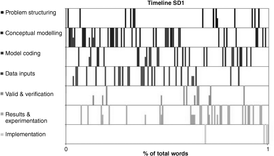
Figure 8.5 Timeline plot for SD1.
The timeline plots (Figures 8.4 and 8.5) are representative of most of those generated with the exception of DES3 and SD5. The former modeller did not complete the model due to difficulties encountered with the large number of attributes and population size. The latter was reluctant to build a model on the computer and so attended to model coding only at the end of the protocol, after being prompted by the researcher.
Observing the DES and SD timeline plots, it is clear that modellers frequently switched their attention to the topics. Similar patterns of behaviour were observed by Willemain (1995), where expert modellers were asked to build models of a generic OR problem. Looking at the overall tendencies in the DES and SD timeline plots, it appears that the DES protocols might follow a more linear progression in the sequence of modelling topics. Linearity of thinking implies that modellers' thinking progresses from the first modelling topics at the top left of the graph to the next one down towards the bottom right corner of the graph, with modelling topics concentrated in the centre of the plot. Meanwhile, in the SD protocols, modellers' attention appears to be more scattered throughout the model building session (Figure 8.5). The transition of attention between modelling topics is further explored in the next subsection.
8.4.3 Pattern of Iterations Among Topics
In this subsection the iterations among modelling topics are explored using transition matrices, with a view to further understanding the pattern of iterations followed by DES and SD modellers. A transition matrix represents the cross-tabulation of the sequence of attention between successive pairs of episodes in a protocol. The total number of transitions occurring in the combined DES and SD protocols is displayed in Table 8.4. It can be observed that DES and SD modellers switched their attention from one topic to another almost to the same extent (505 times for DES modellers and 507 times for SD modellers). In order to explore the dominance of the modellers' thinking, the cells in the transition matrices have been highlighted according to the number of transitions counted. The darker shades represent the transitions that occur most frequently.
Table 8.4 Comparative view of the transition matrices for the combined DES and SD protocols, where each cell has been highlighted depending on the number of transitions.
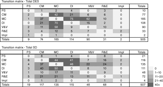 |
The main observations made based on the DES and SD transition matrices are as follows:
- Model coding is the topic DES modellers return to most often (185). Similarly, SD modellers return mostly to model coding.
- The modelling topics that DES modellers alternate between most often are conceptual modelling, model coding, data inputs, and verification and validation (shown by the dark grey highlighted cells in the DES transition matrix in Table 8.4). These transitions form the dominant loop in DES modellers' thinking. Among these transitions the highest are the ones between model coding and data inputs, and vice versa.
- SD modellers alternate mostly in a loop between conceptual modelling, model coding and data inputs. These transitions determine the dominant loop in their thinking process (dark grey highlighted cells in the SD transition matrix in Table 8.4).
- Comparing the dominant loops in the DES and SD transition matrices (Table 8.4), the pattern of the transitions for SD modellers follows a more horizontal progression, while a diagonal progression towards the bottom right-hand side of the matrix is observed for DES modellers. This serves as an indication that DES modellers' thinking process progresses more linearly compared with that of SD modellers.
The indication of linearity identified by comparing the dominant loops in DES and SD modellers' thinking is further verified using the total number of transitions of attention for the parallel linear strips in the two transition matrices. Each parallel strip includes the diagonal row of cells going from the top left to bottom right of the transition matrices (Table 8.4). The cells in each parallel strip have been highlighted in different shades for the DES and SD matrix separately (part (a), Table 8.5). So eight linear strips with different shades have been created, for which the total number of transitions is counted and summed (part (b), Table 8.5). In the case of absolute linear thinking, it is to be expected that all transitions would be concentrated in the central (darkest grey) strip. This would mean that the total number of transitions in the darkest grey strip would be equal to the total number of transitions, that is 505 for DES modellers and 507 for SD modellers. However, this is not the case with any of the DES or SD protocols. Nevertheless, the total number of transitions for all eight linear strips can provide an indication of the extent of linearity involved. The total number of transitions in each corresponding strip is compared for the DES and SD matrices. The highest total of transitions in the most central diagonal strips indicates a more linear modelling process. The highest total of transitions for the strips further away conveys a less linear process. The total number of transitions per linear strip for the DES and SD protocols is shown in Table 8.5(b). The reader should note that the totals shown in Table 8.5(b) differ from the totals in Table 8.4 due to the fact that the cells at the top right and bottom left corners have not been included in a parallel strip.
Table 8.5 Total number of transitions per parallel strip in the DES and SD transition matrices.
 |
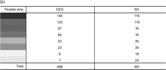 |
Comparing the total number of transitions in each parallel strip for the DES and SD modellers (Table 8.5b), it is observed that for DES modellers the higher numbers are at the top of the table, representing the most central strips in Table 8.5(a). This implies that the transition of attention for DES modellers focuses mainly in the most central strips in the matrix, hence representing a relatively more linear process compared with that for SD modellers. However, for SD modellers it can be observed that the higher totals are found at the bottom of the table, representing cells furthest away from the centre strips in Table 8.5(a). This suggests that the SD modellers switched their attention in a more vertical pattern compared with the DES modellers. It should be noted that an almost equal total number of transitions among topics has been found for DES and SD modellers. Based on the comparison of the transitions per linear strip, it can be concluded that DES modellers' attention progresses relatively more linearly among modelling topics than that of SD modellers.
8.5 Observations from the DES and SD Expert Modellers' Behaviour
Understanding the details of the models developed by each expert modeller is not the primary objective of the analysis presented in this chapter. Nor is a detailed analysis of the modellers' behaviour. However, it is considered beneficial to provide a brief overview of the models developed and some key observations (mostly relevant to the model development process), made while the DES and SD expert modellers undertook the modelling exercise. The following paragraphs give the reader a general idea of the data obtained from the VPA sessions and their richness, but these are by all means not exhaustive.
The prison models developed by the DES and SD experts were simple and hence only small differences could be depicted among them. The modellers started from the basic diagram provided (Figure 8.2) and the majority kept close to the brief. The resulting models provided almost similar numerical results for the base scenario, taking into account in some cases mistakes in data inputs or incorrect computations. Most DES modellers produced tidier models more pleasing to the eye compared with the equivalent SD models. This could be due to the fact that more SD modellers added further structures to experiment with various scenarios.
Despite the limited differences observed in the models developed, some differences were observed in DES and SD expert modellers' reactions to tackling the case study. Some key observations that the authors found interesting are now considered, but these are not exhaustive. It was observed that DES and SD modellers considered similar modelling objectives, related to creating a tool that projects the output of interest into the future. SD modellers, however, showed a tendency to consider broader aspects of the problem modelled. They also considered objectives beyond projecting the size of the prison population or solving the problem of prison overcrowding, such as reducing the number of criminal acts or reducing the cost incurred by the prison system to society. Furthermore, SD modellers related the objectives of the model to testing policies, whereas DES modellers rarely related the objectives of the model to a comparison of scenarios for various policies.
It was further observed that the development of a conceptual diagram was not a priority for most DES and SD modellers. Due to the nature of the task, the participants were provided with a basic diagram in order to provide a common starting point. Most expert modellers were happy with this simple diagram (Figure 8.2) and hence did not consider creating a conceptual diagram. Some modellers made some sketches on paper, but these did not resemble any formal DES- or SD-like conceptual diagrams. Most DES and SD expert modellers conceptualised at the same time as coding the model on the computer.
While it is believed that feedback is the basic structure of SD models, it was observed that most SD modellers naturally identified the individual causal relationships and less often the feedback effects present in the model. Most SD modellers considered the effect of one variable on another, which is the basis that leads to the identification of feedback effects. On the other hand, DES modellers did not consider any equivalent structures. While conceptualising, DES modellers were most interested in setting up the sequential flow of events in the model rather than considering the effects among them.
Furthermore, it was observed that the DES modellers go through an analytic thinking process when modelling the prison population model. They did not consider the wider issues involved in the prison system, but focused mostly on the individual parts of the model, without considering the wider environmental or social factors that affect the prison system. In contrast, different aspects of systems' thinking were identified in the SD protocols. The SD modellers thought about the context and the wider environment the prison model is part of. They also considered the interrelationships between variables as well as the effects of prison on society, which did not occur in the DES protocols.
Most of the DES and SD modellers were happy with the structure and nature of the data provided in the case study description. The tendency either to change the structure of the model (SD4 and SD5) or to suggest additional structures or variables (SD1, SD2 and SD3) was most common in the case of SD modellers. DES modellers, on the other hand, followed the structure given in the case study with higher fidelity and suggested the addition of more detailed parts or information in the model, such as the representation of the geographic spread of prison buildings across the UK.
Detailed thinking characterised the DES modellers' protocols. The use of labels and attributes given to each individual in the system, the inclusion of conditional coding and specialised functions in the DES models added to the complexity and, therefore, the difficulties encountered during modelling. On the contrary, in the SD protocols no specific indications of detailed complexity were identified. Most SD modellers were happy to look at aggregate numbers or people in the prison system. DES modellers also commented on the problems encountered with the large population of the prison system, whereas SD modellers did not raise any issues about this.
The DES models were almost entirely built on quantitative data such as length of sentence, number of offenders (petty and serious) entering prison, number of prisoners already in the system, and so on. The SD modellers used both quantitative and qualitative data. References to graphical displays were categorised as qualitative data. One such example was the use of data in the form of a graphical display representing the total prison population over time. Similar attitudes towards missing data were observed among the DES and SD group of modellers. In both groups some individuals required additional data inputs, whereas others were willing to make assumptions. As expected, randomness was an important aspect in DES modelling, whereas no references were made to it by SD modellers.
Both DES and SD modellers were concerned with creating accurate models. Contrary to expectations, SD modellers did not refer to model usefulness as a way of validating the model. Both DES and SD modellers showed an interest in the quantitative and qualitative aspects of the results of the models. DES modellers were naturally thinking about more detailed results. SD modellers were keener on developing scenarios for experimentation with their models.
8.6 Conclusions
This chapter presented an empirical study that compares the modelling process followed by DES and SD modellers, by undertaking a quantitative analysis of the verbal protocols. In summary, the findings of this study consist of the following:
- DES modellers focus significantly more on model coding and verification and validation of the model, whereas SD modellers concentrate more on conceptual modelling.
- DES modellers' thinking process progresses more linearly among modelling topics compared with that of SD modellers.
- Both DES and SD modellers follow an iterative modelling process, but their pattern of iteration differs.
- DES and SD modellers switch their attention frequently between topics, and almost to the same extent (505 times for DES modellers and 507 for SD modellers) during the model building exercise.
- The cyclicality of thinking during the modelling task is more distinctive for SD modellers compared with DES modellers.
- The DES and SD models developed and their outcomes did not differ substantially.
- Differences were found in the DES and SD expert modellers' thinking during modelling, in terms of model objectives, feedback effects, the level of complexity and detail of models, data inputs and experimentation.
The findings supported the views expressed in the literature and were on the whole as expected. As with generic OR modelling, both DES and SD consist of iterative modelling processes. A new insight gained from this analysis was that DES modellers' thinking followed a more linear process, whereas for SD modellers it involved more cyclicality. Based on the study presented in this chapter, it is not possible to identify the underlying reason that causes DES modellers to follow a relatively more linear process. In order to identify whether this is a result of the nature of the modelling approach used or of the modellers' way of thinking, it would be useful to observe DES modellers building SD models and vice versa.
As expected, differences were identified in the attention paid to different modelling stages. The authors believe that this finding is partly a result of the fact that DES modellers naturally tend to pay more attention to model coding and partly because it is inherently harder to code in DES modelling. Clearly, the results are dependent to some extent on the case study used and the modellers selected. Therefore, considerations need to be made about the limitations of the study and the consequent validity of the findings.
Obviously, it should be noted that the findings of this study are based on the researcher's interpretation of participants' verbalisations. Subjectivity is involved in the analysis of the protocols, as well as in the choice of the coding scheme. A different researcher might have reached different conclusions (using a different coding scheme with different definitions). In order to mitigate the problem of subjectivity, the protocols were coded three times, involving a third party in one case. Additionally, the current findings are based on the verbalisations obtained from a specific sample of modellers who were chosen by convenience sampling. A bigger sample size could have provided more representative results, but due to project timescales this was not feasible. In this study only one case study was used. For future research, the use of more case studies could provide more representative results regarding the differences between the two modelling approaches.
Considering the data (verbal protocols) obtained from the modelling sessions implemented, these are derived from artificial laboratory settings, where the modellers at times felt the pressure of time or the pressure of being observed. The task given to the participants was a simple and quite structured task to ensure completion of an exercise in a limited amount of time. These factors have to some extent affected the smaller amount of verbalisations for modelling topics such as problem structuring, results and experimentation, and implementation. Future research could involve less structured tasks or tasks that introduce more experimentation, whereas implementation is more problematic for a laboratory setting.
This chapter compares the behaviour of expert DES and SD modellers when building simulation models. The findings presented ultimately contribute to the comparison of the two simulation approaches. The main contribution of this study lies in its use of empirical data, gained from experimental exercises involving expert modellers themselves, to compare the DES and SD model building processes. The chapter focuses on a quantitative description of expert modellers' thinking process, analysing the processes that DES and SD modellers think about while building simulation models. It is suggested that the modelling processes followed in DES and SD modelling differ. The observations made during the modelling process suggest a number of differences in the approach taken in different stages of modelling.
For further work the analysis presented here could be extended by undertaking an in-depth qualitative analysis of the 10 verbal protocols. This would enable a more detailed examination of the protocols for each modelling topic so that differences and similarities in the underlying thought processes between DES and SD modellers can be identified. This list of differences and similarities can in turn be linked to specific criteria relevant to the problem characteristics that are to be modelled. This can help in developing a set of criteria that can guide the choice between the two modelling approaches. Future work could also concentrate on developing a framework for supporting the choice between DES and SD for a specific modelling study.
Acknowledgements
The authors would like to thank Suchi Collingwood for her help with the coding of the protocols and who patiently undertook the third blind check of the 10 coded protocols.
Note
References
- Artamonov, A. (2002) Discrete-event simulation vs. system dynamics: comparison of modelling methods. MSc dissertation. Warwick Business School, University of Warwick, Coventry.
- Baines, T.S., Harrison, D.K., Kay, J.M. and Hamblin, D.J. (1998) A consideration of modelling techniques that can be used to evaluate manufacturing strategies. International Journal of Advanced Manufacturing Technology, 14 (5), 369–375.
- Bard, J.F. (1978) The use of simulation in criminal justice policy evaluation. Journal of Criminal Justice, 6 (2), 99–116.
- Brailsford, S. and Hilton, N. (2001) A comparison of discrete-event simulation and system dynamics for modelling healthcare systems. Proceedings of the 26th Meeting of the ORAHS Working Group 2000, Glasgow Caledonian University, Glasgow, Scotland, pp. 18–39.
- Chi, M. (1997) Quantifying qualitative analyses of verbal data: a practical guide. Journal of the Learning Sciences, 6 (3), 271–315.
- Cox, G.B., Harrison, P. and Dightman, C.R. (1978) Computer simulation of adult sentencing proposals. Evaluation and Program Planning, 1 (4), 297–308.
- Coyle, R.G. (1985) Representing discrete-events in system dynamics models: a theoretical application to modelling coal production. Journal of the Operational Research Society, 36(4), 307–318.
- Ericsson, K.A. and Simon, H.A. (1984) Protocol Analysis: Verbal Reports as Data, MIT Press, Cambridge, MA.
- Grove, P., MacLeod, J. and Godfrey, D. (1998) Forecasting the prison population. OR Insight, 11 (1), 3–9.
- Hillier, F.S. and Lieberman, G.J. (1990) Introduction to Operations Research, 5th edn, McGraw-Hill, New York.
- Korporaal, R., Ridder, A., Kloprogge, P. and Dekker, R. (2000) An analytic model for capacity planning of prisons in the Netherlands. Journal of the Operational Research Society, 51 (11), 1228–1237.
- Kwak, N.K., Kuzdrall, P.J. and Schniederjans, M.J. (1984) Felony case scheduling policies and continuances – a simulation study. Socio-Economic Planning Sciences, 18 (1), 37–43.
- Lane, D.C. (2000) You just don't understand me: models of failure and success in the discourse between system dynamics and discrete-event simulation. LSE OR Dept, Working Paper 00.34:26.
- Law, A.M. (2007) Simulation Modeling and Analysis, 4th edn, McGraw-Hill, Boston, MA.
- Mak, H.-Y. (1993) System dynamics and discrete-event simulation modelling. PhD thesis. London School of Economics and Political Science.
- McKelvie, D., Hadjipavlou, S., Monk, D. et al. (2007) The use of SD methodology to develop services for the assessment and treatment of high risk serious offenders in England and Wales. Proceedings of the 25th International Conference of the System Dynamics Society, Boston, MA.
- Meadows, D.H. (1980) The unavoidable a priori, in Elements of the System Dynamics Methods (ed. J. Randers.) Productivity Press, Cambridge.
- Miles, M.B. and Huberman, A.M. (1994) Qualitative Data Analysis: An Expanded Sourcebook, Sage, Thousand Oaks, CA.
- Morecroft, J.D.W. and Robinson, S. (2005) Explaining puzzling dynamics: comparing the use of system dynamics and discrete-event simulation. Proceedings of the 23rd International Conference of the System Dynamics Society, Boston, MA.
- Oral, M. and Kettani, O. (1993) The facets of the modeling and validation process in operations research. European Journal of Operational Research, 66 (2), 216–234.
- Patrick, J. and James, N. (2004) Process tracing of complex cognitive work tasks. Journal of Occupational and Organizational Psychology, 77 (2), 259–280.
- Pidd, M. (2004) Computer Simulation in Management Science, 5th edn, John Wiley & Sons, Ltd, Chichester.
- Randers, J. (1980) Elements of the System Dynamics Method, MIT Press, Cambridge, MA.
- Robinson, S. (2001) Soft with a hard centre: discrete-event simulation in facilitation. Journal of the Operational Research Society, 52 (8), 905.
- Robinson, S. (2004) Simulation: The Practice of Model Development and Use, John Wiley & Sons, Ltd, Chichester.
- Robinson, S. (2005) Discrete-event simulation: from the pioneers to the present, what next? Journal of the Operational Research Society, 56 (6), 619–629.
- Senge, P.M. (1990) The Fifth Discipline: The Art and Practice of the Learning Organisation, Random House, London.
- Sheskin, D.J. (2007) Handbook of Parametric and Nonparametric Statistical Procedures, 4th edn, Chapman & Hall/CRC Press, Boca Raton, FL.
- Sterman, J. (2000) Business Dynamics: Systems Thinking and Modeling for a Complex World, Irwin/McGraw-Hill, Boston, MA.
- Sweetser, A. (1999) A comparison of system dynamics and discrete-event simulation. Proceedings of the 17th International Conference of the System Dynamics Society and 5th Australian & New Zealand Systems Conference, Wellington, New Zealand.
- Tako, A.A. and Robinson, S. (2009) Comparing discrete-event simulation and system dynamics: users' perceptions. Journal of the Operational Research Society, 60, 296–312.
- Todd, P. and Benbasat, I. (1987) Process tracing methods in decision support systems research: exploring the black box. MIS Quarterly, 11 (4), 493–512.
- Willemain, T.R. (1994) Insights on modeling from a dozen experts. Operations Research, 42(2), 213–222.
- Willemain, T.R. (1995) Model formulation: what experts think about and when. Operations Research, 43 (6), 916–932.
- Willemain, T.R. and Powell, S.G. (2006) How novices formulate models. Part II: a quantitative description of behaviour. Journal of the Operational Research Society, 58 (10), 1271–1283.
- Wolstenholme, E.F. (1990) System Enquiry: A System Dynamic Approach, John Wiley & Sons, Ltd, Chichester.