12
Multi-Method Modelling: AnyLogic
Andrei Borshchev
Managing Director and CEO, The AnyLogic Company, St Petersburg, Russia
The three modelling methods, or paradigms, that exist today are essentially the three different viewpoints the modeller can take when mapping the real-world system to its image in the world of models. The system dynamics (SD) paradigm suggests abstracting away from individual objects, thinking in terms of aggregates (stocks, flows) and feedback loops. The discrete-event (DE) modelling paradigm adopts a process-oriented approach: the dynamics of the system are represented as a sequence of operations performed over entities. In an agent-based (AB) model the modeller describes the system from the point of view of individual objects that may interact with each other and with the environment.
Depending on the simulation project goals, the available data, and the nature of the system being modelled, different problems may call for different methods. Also, sometimes it is not clear at the beginning of the project which abstraction level and which method should be used. The modeller may start with, say, a highly abstract system dynamics model and switch later to a more detailed discrete-event model. Or, if the system is heterogeneous, the different components may be best described by using different methods. For example, in the model of a supply chain that delivers goods to a consumer market, the market may be described in (SD) terms, the retailers, distributors, and producers may be modelled as agents, and the operations inside those supply chain components may be modelled as process flowcharts.
AnyLogic meets this challenge by supporting all three modelling methods on a single, modern object-oriented platform. With AnyLogic, a modeller can choose from a wide range of abstraction levels, can efficiently vary them while working on the model, and can combine different methods into one model.
In this chapter we offer an overview of the most used multi-method model architectures, discuss the technical aspects of linking different methods within one model, and consider three examples of multi-method models, namely:
- consumer market and supply chain
- epidemic and clinic
- product portfolio and investment policy.
The example models are described at a very detailed level so that they can easily be reproduced in AnyLogic development environment.
12.1 Architectures
The number of possible multi-method model architectures is infinite, and many are used in practice. Popular examples are shown in Figure 12.1. We will briefly discuss the problems where these architectures may be useful.
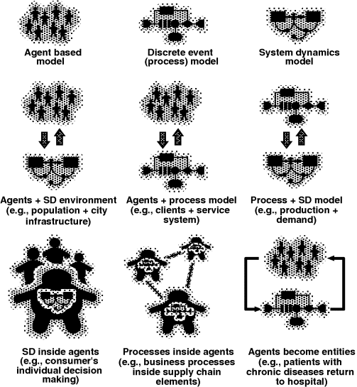
Figure 12.1 Popular multi-method model architectures.
Agents in a SD environment. Think of a demographic model of a city. People work, go to school, own or rent homes, have families, and so on. Different neighbourhoods have different levels of comfort, including infrastructure and ecology, cost of housing, and jobs. People may choose whether to stay or move to a different part of the city, or move out of the city altogether. People are modelled as agents. The dynamics of the city neighbourhoods may be modelled in a SD way, for example, the house prices and the overall attractiveness of the neighbourhood may depend on crowding, and so on. In such a model, agents' decisions depend on the values of the SD variables, and agents, in turn, affect other variables.
The same architecture is used to model the interaction of public policies (SD) with people (agents). Examples are: a government effort to reduce the number of insurgents in society; policies related to drug users or alcoholics.
Agents interacting with a process model. Think of a business where the service system is one of the essential components. It may be a call centre, a set of offices, a Web server or an IT infrastructure. As the client base grows, the system load increases. Clients who have different profiles and histories use the system in different ways, and their future behaviour depends on the response. For example, low-quality service may lead to repeated requests, and, as a result, frustrated clients may stop being clients. The service system is naturally modelled in a discrete-event style as a process flowchart where requests are the entities and where operators, tellers, specialists, and servers are the resources. The clients who interact with the system are the agents who have individual usage patterns.
Note that in the previous example the agents can be created directly from the company CRM database and acquire the properties of the real clients. This also applies to the modelling of the company's HR dynamics. You can create an agent for every real employee of the company and place them in the SD environment that describes the company's integral characteristics (the first architecture type).
A process model linked to an SD model. The SD aspect can be used to model the change in the external conditions for an established and ongoing process: demand variation, raw material pricing, skill level, productivity, and other properties of the people who are part of the process.
The same architecture may be used to model manufacturing processes where part of the process is best described by continuous time equations – for example, tanks and pipes, or a large number of small pieces that are better modelled as quantities rather than as individual entities. Typically, however, the rates (time derivatives of stocks) in such systems are piecewise constants, so simulation can be done analytically, without invoking numerical methods.
SD inside agents. Think of a consumer market model where consumers are modelled individually as agents, and the dynamics of consumer decision making are modelled using the SD approach. Stocks may represent the consumers' perception of products, individual awareness, knowledge, experience, and so on. Communication between the consumers is modelled as discrete events of information exchange.
A larger-scale example is interaction of organisations (agents) whose internal dynamics are modelled as stock and flow diagrams.
Processes inside agents. This is widely used in supply chain modelling. Manufacturing and business processes, as well as the internal logistics of suppliers, producers, distributors, and retailers, are modelled using process flowcharts. Each element of the supply chain is at the same time an agent. Experience, memory, supplier choice, emerging network structures, orders, and shipments are modelled at the agent level.
Agents temporarily act as entities in a process. Consider patients with chronic diseases who periodically need to receive treatment in a hospital (sometimes planned, sometimes because of acute phases). During treatment, the patients are modelled as entities in the process. After discharge from the hospital, they do not disappear from the model, but continue to exist as agents with their diseases continuing to progress until they are admitted to hospital again. The event of admission and the type of treatment needed depend on the agent's condition. The treatment type and timeliness affect the future disease dynamics.
There are models where each entity is at the same time an agent exhibiting individual dynamics that continue while the entity is in the process, but are outside the process logic – for example, the sudden deterioration of a patient in a hospital.
12.1.1 The Choice of Model Architecture and Methods
AnyLogic, designed as a multi-method object-oriented tool, allows you to create model architectures of any type and complexity, including those previously mentioned. You can develop complex, simple, flat, hierarchical, replicated, static, or dynamically changing structures.
The choice of the model architecture depends on the problem you are solving. The model structure reflects the structure of the system being modelled – not literally, however, but as seen from the problem viewpoint. The choice of modelling method should be governed by the criterion of naturalness. Compact, minimalistic, clean, beautiful, easy to understand, and explain – if the internal texture of your model is like that, then you have chosen the right method.
12.2 Technical Aspect of Combining Modelling Methods
In this section we will consider the techniques of linking different modelling methods in AnyLogic.
The very first thing you should know is that all model elements of all methods, be they SD variables, statechart states, entities, process blocks, and even animation shapes or business charts, exist in the “same namespace”: any element is accessible from any other element by name (and, sometimes, “path” – the prefix describes the location of the element).
The following examples are all taken from real projects and purged of all unnecessary details. This set, of course, does not cover everything, but it does give a good overview of how you can build interfaces between different methods.
12.2.1 System Dynamics → Discrete Elements
The SD model is a set of continuously changing variables. All other elements in the model work in discrete time (all changes are associated with events). SD itself does not generate any events, so it cannot actively have an impact on agents, process flowcharts, or other discrete-time constructs. The only way for the SD part of the model to affect a discrete element is to let that element watch a condition over SD variables, or to use SD variables when making a decision. Figure 12.2 shows some possible constructs.
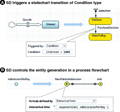
Figure 12.2 SD impacts discrete elements of the model.
In case A, SD triggers a statechart transition. Events (low-level constructs that allow scheduling a one-time or recurrent action) and statechart transitions are frequent elements of agent behaviour. Among other types of triggers, both can be triggered by a condition – a Boolean expression.
If the model contains dynamic variables, all conditions of events and statechart transitions are evaluated at each integration step, which ensures that the event or transition will occur exactly when the (continuously changing) condition becomes true.
In Figure 12.2A the statechart is waiting for the Interest to rise higher than a given threshold value. The statechart can be located on the same level as the SD, or in a different active object.
In case B the source block NewPatientAdmission generates new entities at the rate defined by the dynamic variable AdmissionsPerDay. The arrivals are defined in the form of interarrival time and not in the form of rate, because the rate is not re-evaluated during the simulation, whereas the interarrival time is re-evaluated after each new entity.
Note that if the value of the dynamic variable changes in between two subsequent event occurrences (or in between two entity arrivals), this will not be “noticed” immediately, but only at the next event occurrence (or next entity arrival).
12.2.2 Discrete Elements → System Dynamics
For cases C–E below, see Figure 12.3.
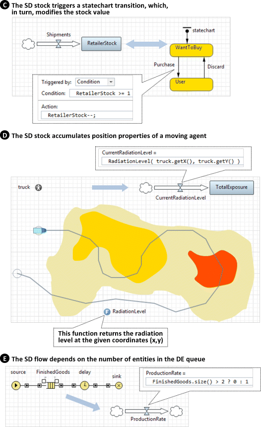
Figure 12.3 Discrete elements of the model impact SD.
In case C, the SD stock triggers a statechart transition, which, in turn, modifies the stock value. Here, the interface between the SD and the statechart is implemented in the pair condition/action. In the state WantToBuy, the statechart tests if there are products in the retailer stock and, if there are, buys one and changes the state to User.
In case D, the SD stock accumulates the “history” of the agent motion. This is an interesting example of SD–AB cooperation. The value of the stock TotalExposure is constantly updated as the mobile agent moves through the area contaminated by radiation. The value of the incoming flow CurrentRadiationLevel is set to the radiation level at the coordinates of the truck agent. As the truck moves or stays, the stock receives and accumulates a dose of radiation per time unit. Again, in the SD equation, we are referencing the agent and calling its function.
In case E, referencing DE objects in the SD formula, the flow ProductionRate switches between 0 and 1, depending on whether the finished products' inventory (the number of entities in the queue FinishedGoods returned by the function size()) is greater than 2 or not. Again, one can close the loop by letting the SD part control the production process.
12.2.3 Agent Based ↔ Discrete Event
For cases F and G below, see Figure 12.4.
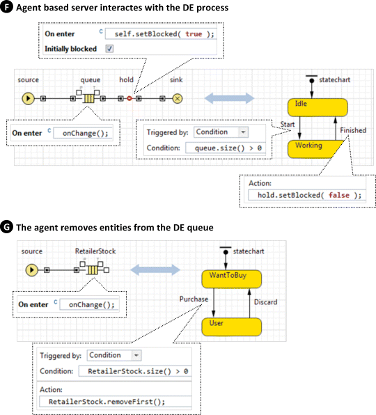
Figure 12.4 Agent-based parts of the model interact with discrete-event parts.
In case F, a server in the DE process model is implemented as an agent. Consider some complex equipment, such as a robot or a system of bridge cranes. The behaviour of such objects is often best modelled “in agent-based terms” by using events and statecharts. If the equipment is part of the manufacturing process being modelled, you need to build an interface between the process and the agent representing the equipment.
In this example, the statechart is a simplified equipment model. When the statechart comes to the state Idle, it checks if there are entities in the queue. If so, it proceeds to the Working state and, when the work is finished, unblocks the hold object, letting the entity exit the queue. The hold object is set up to block itself again after the entity passes through.
The next entity will arrive when the equipment is in the Idle state. To notify the statechart, we call the function onChange() upon each entity arrival (see the On enter action of the queue).
In case G, the agent removes entities from the DE queue. Here, the supply chain is modelled using DE constructs; in particular, its end element, the retailer stock, is a queue object. The consumers are outside the DE part and are modelled as agents. Whenever a consumer comes to the state WantToBuy, it checks the RetailerStock and, if it is not empty, removes one product unit. Again, as this is a purely discrete model, we need to ensure that the consumers who are waiting for the product are notified about its arrival – that is why the code onChange() is placed in the On enter action of the RetailerStock queue.
12.3 Example: Consumer Market and Supply Chain
We will model the supply chain and sales of a new product in a consumer market in the absence of competition. The supply chain will include delivery of the raw product to the production facility, production, and the stock of finished products. The QR inventory policy will be used. Consumers are initially unaware of the product; advertising and word of mouth will drive the purchase decisions. The product has a limited lifetime, and 100% of users will be willing to buy a new product to replace the old one.
We will use DE methodology to model the supply chain, and SD methodology, namely, a slightly modified Bass diffusion model (Bass, 1969), to model the market. We will link the two models through the sales events.
12.3.1 The Supply Chain Model
The supply chain flowchart (see Figure 12.5) includes three stocks (the supplier stock of raw material, the stock of raw material at the production site, and the stock of finished products at the same location). Delivery and production are modelled by the two Delay objects with limited capacity. The delay time for both has been left at the default value of triangular(0.5, 1, 1.5). To load the supply chain with some initial product quantity we will add this StartUp code:
Supply.inject( OrderQuantity);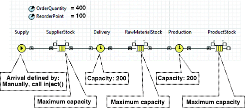
Figure 12.5 The discrete-event model of the supply chain.
If we run this model, at the beginning of the simulation 400 items of the product are produced and accumulate in the ProductStock. Nothing else happens in the model (the Supply object is set up to not generate any new entities, unless explicitly asked to do so). The inventory policy is not yet present in our model.
12.3.2 The Market Model
The market is modelled by an SD stock and flow diagram as shown in Figure 12.6. The SD part is located in the Main object – just on the same canvas where the flowchart was created earlier. The difference of our market model from the classical Bass diffusion model with discards (Sterman, 2000) is that the users', or adopters', stock of the classical model is split into two: the Demand stock and the actual Users stock. The adoption rate in this model is called PurchaseDecisions. It brings PotentialUsers not directly into the Users stock, but into the intermediate stock Demand, where they wait for the product to be available. The actual event of sale, that is, the “meeting” of the product and the customer who wants to buy it, will be modelled outside the SD paradigm.
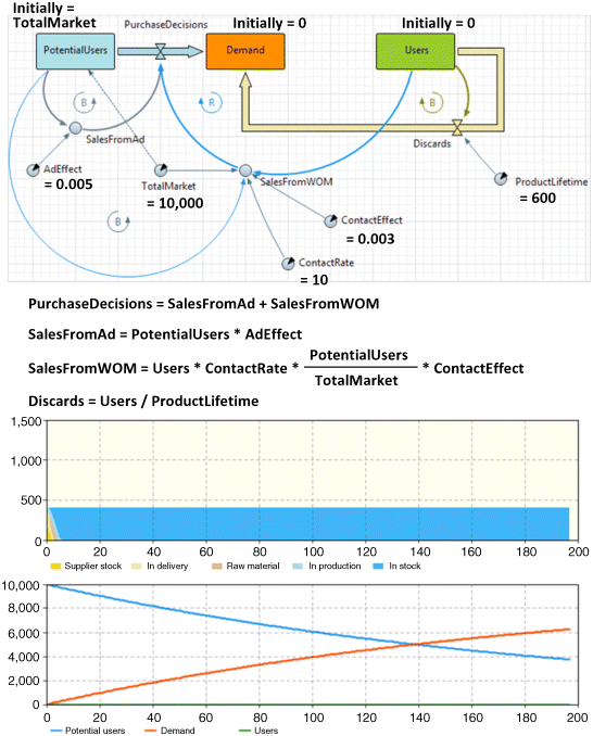
Figure 12.6 The SD model of the market; the dynamics of the unlinked model.
The two pieces of the model are not yet linked. If we run the model, the supply chain will still produce the 400 items and stop, and the potential clients will gradually make their purchase decisions, building up the Demand stock. Note that in the current version of the model, the only reason for the potential users to make a purchase decision is advertising. The word-of-mouth effect is not yet working because nobody has actually purchased a single product item. To better view the model dynamics in future experiments, it makes sense to add a couple of charts as shown in Figure 12.6.
12.3.3 Linking the DE and the SD Parts
How do we link the supply chain and the market? We want to achieve the following:
- If there is at least one product item in stock and there is at least one client who wants to buy it, the product item should be removed from the ProductStock queue, the value of Demand should be decremented, and the value of Users should be incremented, see Figure 12.7.
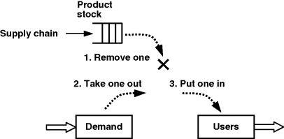
Figure 12.7 Linking the supply chain and the market: the scheme.
We therefore have a condition and an action that should be executed when the condition is true. The AnyLogic construct that does exactly that is the condition-triggered event. The implementation of our scheme in the AnyLogic modelling language is shown in Figure 12.8.
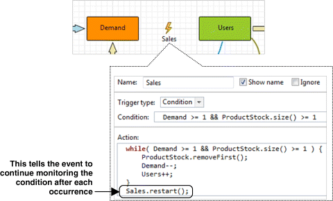
Figure 12.8 Linking the supply chain and the market: the implementation.
A couple of comments on how the condition-triggered events work are in order:
We put the sale into a while loop, because a possibility exists that two or more product items may become available simultaneously, or the Demand stock may grow by more than one unit per numeric step. Therefore, more than one sale can potentially be executed per event occurrence.
12.3.4 The Inventory Policy
With the Sales event in place, sales start to happen. The 400 items produced at the beginning of the simulation disappear in about a week. The Users stock increases up to almost 400; it then slowly starts to decrease according to our limited lifetime assumption. And, since we have not yet implemented our inventory policy, no new items are produced. This is the last missing piece of the model. We will include the inventory policy in the same Sales event; the inventory level will be checked after each sale.
We will modify the Action of the Sales event this way:
while( Demand >= 1 && ProductStock.size() >= 1) {//execute saleProductStock.removeFirst(); //remove a product unit from the stock (DE)Demand--; //remove a waiting client from Demand stock (SD)Users++; //add a (happy) client to the Users stock (SD)}//apply inventory policyint inventory = //calculate inventoryProductStock.size() + //in stockProduction.size() + //in productionRawMaterialStock.size() + //raw product inventoryDelivery.size() + //raw product being deliveredSupplierStock.size(); //supplier's stockif( inventory < ReorderPoint) //QR policySupply.inject( OrderQuantity);//continue monitoringSales.restart();
Now, the supply chain starts to work as planned, see Figure 12.9. (Here the inventory chart and the market charts are combined: one was dragged onto the top of the other, and the labels were put on different sides.)
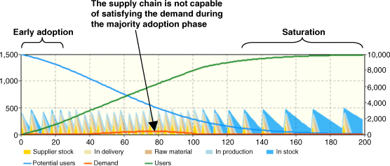
Figure 12.9 The supply chain dynamics pattern changes as the market gets saturated.
During the early adoption phase the supply chain performs adequately, but as the majority of the market starts buying, the supply chain cannot keep up with the market. In the middle of the new product adoption (days 40–100), even though the supply chain works at its maximum throughput, the number of waiting clients still remains high. As the market becomes saturated, the sales rate reduces to the replacement purchases rate, which equals the Discard rate in the completely saturated market, that is, TotalMarket/ProductLifetime = 16.7 sales per day. The supply chain handles that easily.
An interesting exercise would be to make the supply chain adaptive. You can try to minimise the order backlog and at the same time minimise the inventory by adding the feedback from the market model to the supply chain model.
12.4 Example: Epidemic and Clinic
We will create a simple AB epidemic model and link it to a simple DE clinic model. When a patient discovers symptoms, he will ask for treatment at the clinic, which has limited capacity. We will explore how the capacity of the clinic affects the disease dynamics. This model was suggested in 2012 by Scott Hebert, a consultant at AnyLogic North America.
12.4.1 The Epidemic Model
We will add the Agent Population to the editor of Main (the object that is created by default with the new model). The agents will be our patients; their initial number is 2000. We will place the agents into a rectangular area of 650 by 200 miles (1040 by 320 km) and create a distance-based network; two patients are connected if they live at most 30 miles (48 km) away.
The next step is to define the behaviour of our patient. In the Patient object we will create a statechart. The statechart (see Figure 12.10) is similar to the classical SEIR statechart (Wikipedia, 2013). The patient is initially in the Susceptible state, where he can be infected. Disease transmission is modelled by the message "Infection" sent from one patient to another. Having received such a message, the patient transitions to the state Exposed, where he is already infectious, but does not have symptoms. After a random incubation period, the patient discovers symptoms and proceeds to the Infected state. We distinguish between the Exposed and Infected states because the contact behaviour of the patient is different before and after he discovers symptoms: the contact rate in the Infected state is 1 per day, as opposed to 5 in the Exposed state. The internal transitions in both states model contacts. We model only those contacts that result in disease transmission; therefore, we multiply the base contact rate by Infectivity, which, in our case, is 7%.

Figure 12.10 The patient behaviour statechart.
There are two possible exits from the Infected state. The patient can be treated in a clinic (and then he is guaranteed to recover), or the illness may progress naturally without intervention. In the latter case, the patient can still recover with a high probability (90%), or die. If the patient dies, he is deleted from the model, see the Action of the Dead state. The completion of treatment is modelled by the message "Treated" sent to the agent. So far, this message is never received, because we have not yet created the clinic model.
The recovered patient acquired a temporary immunity to the disease. We reflect this in the model by having the state Recovered, where the patient does not react to the message "Infection" that may possibly arrive. At the end of the immunity period the transition ImmunityLost takes the patient back to the Susceptible state.
Note that as long as we have defined the parameters inside the agent, we can make their values different for different agents. In our model, however, for simplicity they are the same throughout the whole population.
For animation purposes, we will paint the patient differently, depending on his state. In the Entry action field of each state, we will type the code that changes the colour of the patient animation into the colour of the state, for example, in the Entry action of the state Exposed we will type: person.setFillColor(darkOrange);.
And finally, we need to create the initial entry of the infection into the population. In the StartUp code field of the Main object we will type the following code:
for( int i=0; i<5; i++)patients.random().receive( "Infection");
This will infect five randomly chosen people at the beginning of the simulation.
Now we can run the epidemic model. Look at the top of Figure 12.11. The contagious disease spreads around the initially infected agents (remember that our network of contacts is based on distance). The epidemic does not end after the first wave, because the immunity period is not long enough. We will add a chart to view the type of SD.

Figure 12.11 Oscillation in the epidemic model.
AnyLogic supports the collection of statistics on agent populations. We will define four statistics in the patient population. The first one will be called NSusceptible and will count the patients for which the condition item.statechart.isStateActive(item.Susceptible) evaluates to true. Similarly, we will count all exposed, infected, and recovered patients. We will use the AnyLogic Time stack chart with a time window of 500 days to display the statistics. At the bottom of Figure 12.11 you can see the oscillation and gradual decrease of the total population due to deaths.
12.4.2 The Clinic Model and the Integration of Methods
The next step is to add the clinic, and let the patients be treated there. Our clinic will be modelled via a very simple DE model: the Queue for the patients waiting to be treated and the Delay modelling the actual treatment.
We will put the process flowchart (see Figure 12.13A) in the Main object. Unlike in classical DE models, however, the entities in this process are not generated by a Source object, but are injected by the agents via an Enter object. The communication scheme between the patients–agents and the clinic process is shown in Figure 12.12.
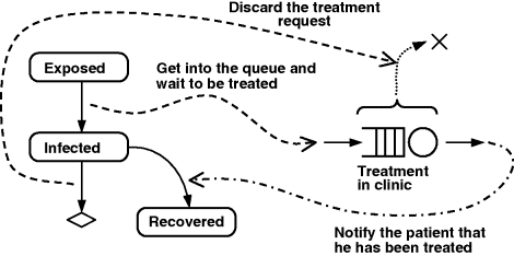
Figure 12.12 Interface between the agent-based and the discrete-event parts of the model.
Once the patient discovers symptoms, he creates an entity – let's call it “treatment request” – and injects the entity into the clinic process. Once the treatment is completed, the entity notifies the patient by sending him a message “Treated” that causes the patient to transition to the Recovered state. If, however, the patent is cured or dies before the treatment is completed, he will discard his treatment request by removing it from whatever stage it is at in the process. On the technical side, we need:
- The entity that will carry the reference to the patient.
- The ability to remove the entity originated by a particular patient from the process.
We will create a custom entity class TreatmentRequest that has a field patient – this will be the reference to the patient (agent) who originated the treatment request. In the process flowchart (Figure 12.13A), we identified that the entities passing through the wait, treatment, and finished objects are not of the generic Entity class, but of its subclass TreatmentRequest. This is necessary because we plan to use the patient field of those entities. For example, when the treatment is finished, the finished object sends a message “Treated” to the patient referenced by the entity before disposing of the entity.
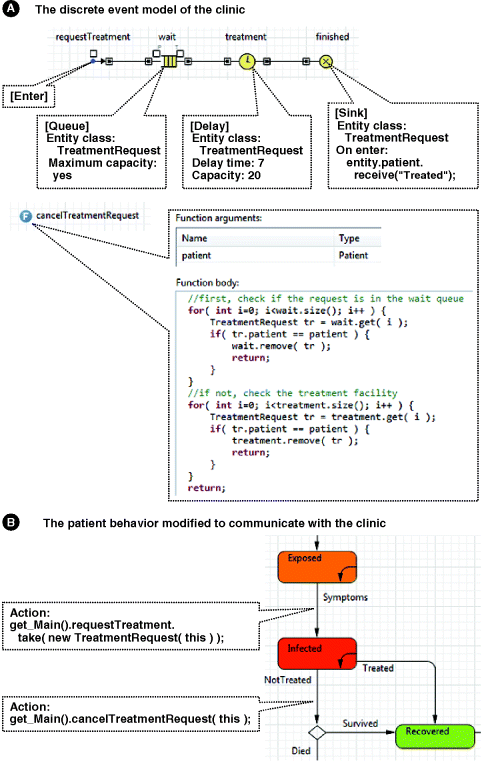
Figure 12.13 The discrete-event model of the clinic and integration with the agent-based model.
We also specified that the queue has infinite capacity, that the treatment takes exactly seven days, and that there are only 20 beds in the clinic, so only 20 patients can be treated simultaneously.
Also, we prepared the function cancelTreatmentRequest() that will be called by patients who got well on their own or died before getting the chance to be treated. That function uses the API (Application Programming Interface) of the Queue and Delay objects to search for a particular entity in them and remove it.
The remaining task is to modify the behaviour of Patient to link it to the model of clinic. We will add the actions to the statechart transitions Symptoms and NotTreated as shown in Figure 12.13B. Remember that since the clinic process is located one level above the patient's statechart, in the Main object, the clinic objects and functions should be preceded by the prefix get_Main(). The Java word "this" references the object to which the code belongs, in this case the patient. The model is complete.
Now the model shows a different dynamic or, to be more precise, a different range of dynamics. The oscillations are still possible, but a possibility also exists that the epidemic will end after the first wave, as you can see in Figure 12.14. You may experiment with different clinic capacities to figure out the number of beds needed in order to treat everybody on time and prevent further waves of the epidemic.
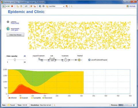
Figure 12.14 The behaviour of the integrated model.
12.5 Example: Product Portfolio and Investment Policy
A company develops and sells consumer products with a fairly short lifecycle. After the product has been successfully launched, its revenue peaks, and then falls, as shown in Figure 12.15. To keep the business going the company has to maintain a continuous process of new product research and development. Part of the company's revenue is therefore reinvested in R&D, and another significant part is spent on introducing new products. We will investigate how the investment policy affects the business.

Figure 12.15 The product lifecycle and associated costs.
12.5.1 Assumptions
We will make some simplifying assumptions, as follows.
The product lifecycle:
- The duration of the research phase of a product is uniformly distributed between 1.5 and 6 years. During this phase, each product is assigned a random “success factor” which is uniformly distributed between 0 and 1. At the end of the research phase, the product is killed if its success factor is less than 0.5; otherwise, it proceeds to the development phase.
- The duration of the development phase is also uniformly distributed between 1 and 3 years. During the development phase, the initial success factor is modified by adding a random number uniformly distributed between −0.3 and 0.3. At the end of the development phase, the project is killed if its success factor is less than 0.5; otherwise, it is released to the market.
- When the product is launched, its success factor is once again modified by adding a random number between −0.3 and 0.3. This value of the success factor then stays the same. As you can see, the value is between 0.2 and 1.6.
Revenue and cost:
- While in the market, all products have the same curve of base revenue over time (see Figure 12.16), and the actual revenue equals base times the “success factor”.
- The first two years of the product in the market are considered as an “introduction period”. At any time after the introduction period the product is discontinued if its annual revenue falls below $5M.
- The annual cost of research is $0.5M per product and is the same for all products. The annual cost of development is $1M per year. The cost of introducing a new product is $10M, which is spent evenly during the two years. In addition there is a one-time fixed cost of $0.5M for starting a new R&D project.
- After the introduction period we will assume no cost per product in market, in other words, we will treat the revenue as revenue after production and distribution costs.

Figure 12.16 The base revenue curve of a product.
Investment policy:
- A fraction of the company revenue goes into “investment capital.” All R&D costs are paid from the investment capital.
- The company has a limited R&D capacity and cannot perform more than 100 projects concurrently.
- Once the company determines that the accumulated investment capital is greater than (the number of ongoing R&D projects + 1) times the “average project cost” ($3M is assumed), a new project is started.
- The invested fraction of the revenue is determined as follows. If the accumulated investment capital is greater than the R&D capacity times the “average project cost,” no money is invested. Otherwise, 20% of the revenue goes into the investment capital stock.
- The remaining part of the revenue goes into the “main capital” stock, and product introduction costs are paid from there.
Assumptions, as you can see, are quite strong. For example, R&D projects may be killed at only two points, at the end of the research phase and at the end of the development phase, but not halfway through. The money spent on introducing the new product does not vary from product to product, the product lifecycles are similar, and there are no complete market failures and no great, long-lasting successes. All these things can be incorporated into the simulation model, but for the purpose of demonstrating the interaction of different modelling methods a simpler model will work just fine. Of course, all numeric values previously given are not fixed and will become the model parameters.
12.5.2 The Model Architecture
We will model each product individually as an agent (as you know, agents in AB models are not necessarily people – they can be anything), so the product portfolio will be a population of agents. The company finances and investment policy will be a SD component. The overall architecture of the model is shown in Figure 12.17. The product lifecycle is naturally represented as a statechart that starts in the Research state and is deleted from the model when it is discontinued or killed. The implementation of the interface between the products–agents and the SD part will be clear from the step-by-step description that follows.
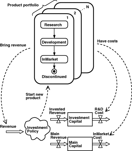
Figure 12.17 Architecture of the product portfolio and investment policy model.
12.5.3 The Agent Product and Agent Population Portfolio
In a new model, we will create an agent population portfolio with agent class Product. The initial population size will be 100. We will use a circle (bubble) as the animation of product. Later we will create a bubble chart, and as the product progresses through the lifecycle phases, its bubble will move.
Product behaviour will be defined in the form of a statechart, see Figure 12.18. The statechart structure straightforwardly reflects the product lifecycle.
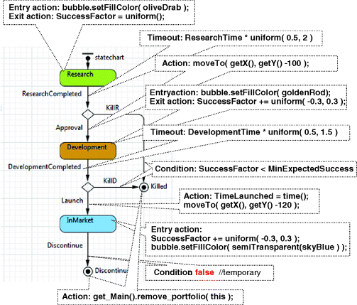
Figure 12.18 Statechart of the agent Product.
Also, the product will have the parameters and variables shown in Figure 12.19. As you can see, the numeric values in the problem statement have become parameters in the model.
For example, the duration of the development phase was originally specified as uniformly distributed between 1 and 3 years. In the model, the parameter DevelopmentTime has an initial value of 2, and in the timeout expression in the DevelopmentCompleted transition, it is multiplied by a random coefficient taking values between 0.5 and 1.5, which gives us the distribution we need. Should we decide to change the average value of the development duration, the resulting interval will correctly follow it.
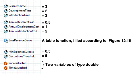
Figure 12.19 Variables, and parameters of the agent Product.
If you run the model at this stage, at the beginning of the simulation you will see 100 olive-coloured bubbles scattered randomly. After a while, some bubbles turn brown and move up, and some disappear; these are the projects that were killed after the research phase. Then, more bubbles disappear, and the rest turn blue and move further up – these are the products that go to market. As the condition of the Discontinue transition is at the moment set to false, the products will remain in the market for ever.
We will now add the cost and revenue calculation to the Product agent, fill in the missing condition, and enhance the animation. The calculation is implemented in the form of three functions at the agent level, see Figure 12.20 (the return type of all functions is double).
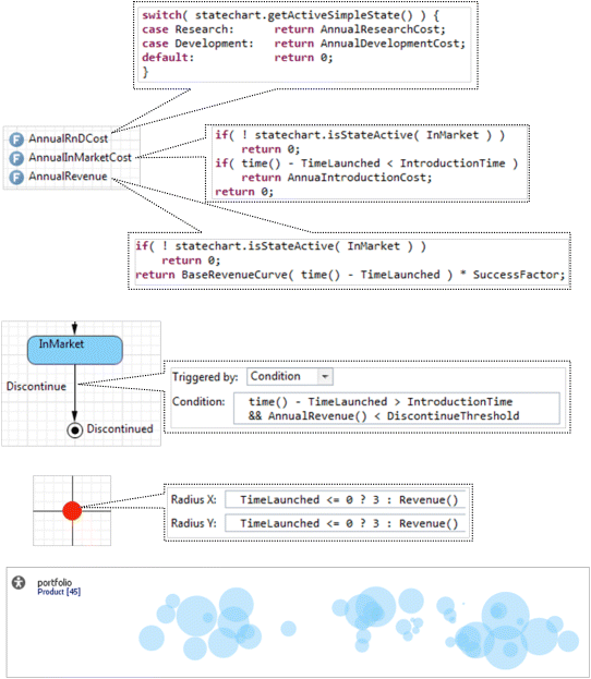
Figure 12.20 Functions calculating cost and revenue. Updated statechart and animation.
The calculations are based on the current state of the product. The statechart functions isStateActive() and getActiveSimpleState() are used to obtain the state. However, while the product is in the market, there is one special state that is not reflected in the statechart, namely, the introduction phase that lasts for two years, according to our specification. To find out whether the product is in the introduction phase, we compare the time from the product launch (time() – TimeLaunched) and IntroductionTime. The time from the launch is also provided as an argument to the table function BaseRevenueCurve().
Now we can add the condition that triggers the Discontinue transition in the product statechart, see the middle fragment of Figure 12.20. The condition reflects the fact that the product can be discontinued only after the introduction phase. We can also enhance the product animation by making the size of the bubble dynamically reflect the revenue brought by the product, see the dynamic expression of the bubble radius.
Now, if you run the model, you can see that the bubbles of the products in the market change their sizes dynamically as the revenue rises and then falls. Eventually, the bubbles seem to disappear.
In fact, the bubbles (and the corresponding products) do not disappear completely, as nobody is telling the agent to recalculate the condition of the Discontinue transition. This will be done by the SD part of the model that we will build next.
12.5.4 The Investment Policy
The next step is to model the company investment policy. This will be done at the Main level. We will create statistical items in the portfolio agent population calculating the total revenue and costs, and use the statistics in the SD model of investment. After that, we will model the start of new R&D projects, which depends on the money accumulated in one of the SD stocks.
The statistics items will be:
- AnnualRevenue – the sum of item.AnnualRevenue() across all products
- AnnualRnDCost – the sum of item.AnnualRnDCost() across all products
- AnnualInMarketCost – the sum of item.AnnualInMarketCost() across all products
- NinRnD – the count of ! item.statechart.isStateActive(item.InMarket) across all products. This is the number of products in the R&D phase.
As a first iteration of the SD part, we will add just one dynamic variable, Revenue, and set its formula to portfolio.AnnualRevenue(). The chart of that variable over time is shown in Figure 12.21. As one might expect, the total revenue of several products launched approximately at the same time is similar to the base revenue curve of a single product. The company is not investing in new product R&D, and in about 15 years it goes out of business.
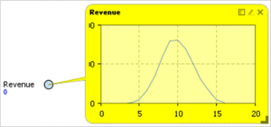
Figure 12.21 Total revenue of several products launched at approximately same time.
Now we will draw the first meaningful draft of the stock and flow diagram of the company's investment policy, see Figure 12.22. If we run the model, we will observe that, shortly after the simulation starts, the InvestmentCapital stock falls down below zero, see the bottom chart in Figure 12.22. It happens because, at the beginning of the simulation, the company starts too many (100) R&D projects simultaneously; they consume money, but bring in no revenue. As the products are launched in the market, the stock goes back up and then follows the S-shaped curve typical of systems with saturation. The MainCapital stock has a slight depression during the products' introduction period and then follows the same S-shaped curve.
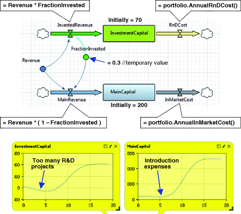
Figure 12.22 The first draft of the SD model of investment policy.
12.5.5 Closing the Loop and Implementing Launch of New Products
In the next step, we will close the loop and implement the rule for starting new products, depending on the available investment money. This will be done by an event StartNewProject at the level of Main.
See Figure 12.23. The parameter AverageProjectCost is an estimation of how much money will be required (per project) to finish all the ongoing projects plus a new one. The event StartNewProject is constantly monitoring the InvestmentCapital stock and, when it detects room for one more project, starts it. The one-time project setup cost is immediately subtracted from the stock, and a new Product agent is created in the portfolio population. The last statement in the event action (the call of the restart() function) tells the event to resume monitoring the condition after each occurrence. Also, because the new products are now created automatically, we will set the initial number of products to 0.
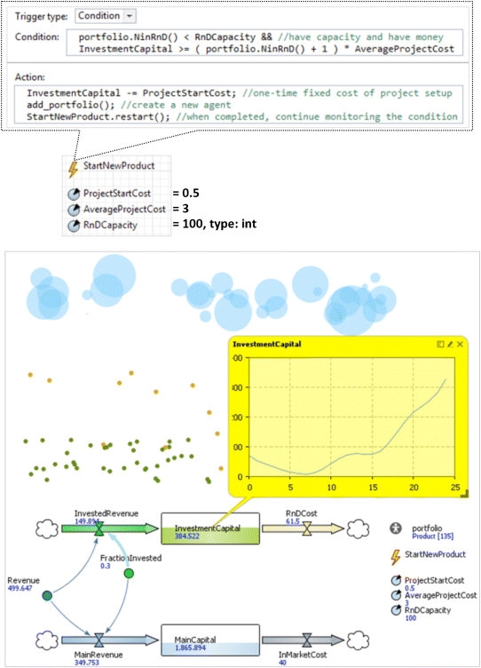
Figure 12.23 Condition event that creates new products. The new dynamics of the model.
Now the company acts safely and is profitable. The continuous R&D process ensures that the company always has new products to offer. The revenue stream grows during the first three decades up to approximately $800M per year and then starts oscillating irregularly around that value. Further revenue growth is limited by the R&D capacity of the company.
12.5.6 Completing the Investment Policy
Under the current model setup, 30% of the company's gross revenue always goes into the investment capital stock, which continues to build up and remains largely unused. In the last step, we will implement the remaining part of the investment policy, that is, we will make the invested fraction of the revenue a variable that depends on the accumulated resources. This is done purely at the SD level by changing the formula of FractionInvested to
InvestmentCapital > RnDCapacity * AverageProjectCost ? 0 : MaxFraction,where MaxFraction is a new model parameter with a default value of 0.2.
The picture is different now (Figure 12.24). The InvestmentCapital stock reaches the value of $300M and stops growing. The revenue oscillates around $800M per year, which, as we know already, is the upper limit with the given R&D capacity.
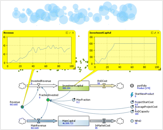
Figure 12.24 Total company dynamics under the fully implemented investment policy.
We can use this model to optimize the investment policy. For example, we can investigate how sensitive the company dynamics are to the parameters of the investment policy, say, to MaxFraction. We will compare the curves of revenue over time obtained in different simulation runs. The results of the sensitivity analysis experiment is shown in Figure 12.25.
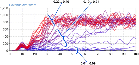
Figure 12.25 Sensitivity analysis: revenue dynamics under different invested fraction values.
The results are interesting. The curves of revenue over time cluster into three groups, as in the figure. In the first one the company goes out business; this corresponds to values of MaxFraction from 0.01 to 0.09. When the parameter is in the range 0.10 to 0.21, the revenue climbs up – the higher the MaxFraction, the faster the maximum value of $800M is reached. Further increase of the invested revenue fraction does not affect the growth.
12.6 Discussion
When developing a DE model of a supply chain, IT infrastructure, or a contact centre, a modeller would typically ask the client to provide the arrival rates of the orders, transactions, or phone calls. The modeller would then be happy to get some constant values, periodic patterns, or trends, and treat arrival rates as variables exogenous to the model. In reality, however, those variables are outputs of another dynamic system, such as a market, a user base. Moreover, this other system can, in turn, be affected by the system being modelled. For example, the supply chain cycle time, which depends on the order rate, can affect the satisfaction level of the client, which impacts repeated orders and, through word of mouth, new orders from other customers. The choice of the model boundary therefore is very important.
The only methodology that explicitly talks about the problem of model boundary is the SD one (Sterman, 2000). However, the SD modelling language is limited by its high level of abstraction, and many problems cannot be modelled with the necessary accuracy. With multi-method modelling one can choose the best-fitting method and language for each component of the model and combine those components while staying on one platform.
For those who would like to continue learning the exciting discipline of multi-method modelling, we can suggest the following exercise:
All models considered in this chapter are available with AnyLogic software and also at the online simulation portal www.RunTheModel.com.
References
- Bass, F. (1969) A new product growth model for consumer durables. Management Science, 15 (5), 215–227.
- Sterman, J.D. (2000) Business Dynamics: Systems Thinking and Modelling for a Complex World, McGraw-Hill, New York.
- Wikipedia (2013) Compartmental models in epidemiology, http://en.wikipedia.org/wiki/Compartmental_models_in_epidemiology.
