15
The Ways Forward: A Personal View of System Dynamics and Discrete-Event Simulation
Michael Pidd
Lancaster Business School, University of Lancaster, UK
15.1 Genesis
In a chapter that speculates on the future, it seems wise to begin by looking backwards to see what we can learn. Both system dynamics and discrete-event simulation have been used for over 50 years. System dynamics, originally christened industrial dynamics by its MIT-based, founding father Jay Forrester, was born in the late 1950s. The first publication had the title ‘Industrial dynamics: a major breakthrough for decision makers’ (Forrester, 1958) and later became the second chapter of the book Industrial Dynamics (Forrester, 1961), which presents and explains the methods and assumptions of what we now refer to as system dynamics. Given Forrester's engineering background it is hardly surprising that system dynamics treats system structure and feedback control as key to system behaviour. Forrester's argument in these early publications promoting industrial dynamics is based on a straightforward analogy between control engineering and organisational behaviour. Forrester (1961) argues that organisations include feedback structures that need to be understood and managed to achieve high performance. Forrester argued that industrial dynamics provided the tools needed to do this.
If the approach now known as system dynamics appeared largely as the result of one man's work, doubtless supported by others, the origins of discrete-event simulation are harder to pin down. According to Hollocks (2006), what we now know as discrete-event simulation was first employed in the UK steel industry in 1957 in the GSP system. The first European text on discrete-event simulation, though it did not use that term, was Tocher (1962) and it is interesting to note that its author regarded computer simulation as a temporary solution to problems that would eventually be solved in mathematical statistics. The year 1962 also saw the publication of the first paper on the GPSS simulation language (Gordon, 1962) in the United States. Variants of GPSS are still in use. Just as Forrester's engineering background is clearly seen in the methods and assumptions of system dynamics, the influence of the discrete-event simulation pioneers is also evident today. Keith Tocher was a pioneer in both statistical methods and computing and it remains true that becoming proficient in the use of discrete-event simulation requires mastery of appropriate statistical methods and a facility with computers.
15.2 Computer Simulation in Management Science
I joined Lancaster University as a young academic in 1979, after a spell at Aston University that was preceded by a job in industry, and was asked to teach simulation methods to undergraduates. I struggled to find a suitable book for the course, mainly because existing ones seemed to me to be out of date. They assumed inflexible mainframe computing, whereas I was using interactive time-shared computing services and personal computers and was convinced that interactive computing was the way ahead. After three years of teaching at Lancaster I was naive enough to think I could write a better and more up-to-date book than those available. I was fortunate to work with some very perceptive colleagues at Lancaster, in particular John Crookes, who argued that PCs (actually Apple II computers at that stage) would fundamentally change how we built and used simulation models. I also discovered word processing on Apple IIs and laboriously used the rather crude Applewriter software to write the text. This allowed the publishers to typeset from disk, which seemed very advanced at the time.
Hence, I wrote my own book, Computer Simulation in Management Science (Pidd, 1984), which stayed in print for 30 years, though heavily revised from time to time and now in its final, fifth, edition. Though it touched the bases needed for simulation on mainframe computers, it emphasised simulation models developed and run using interactive computing. It was, perhaps, rather light on the statistical aspects of discrete-event simulation, mainly because these were covered very well in books by other authors. Unusually, it included both discrete-event simulation and system dynamics in its coverage; a lead that few authors have chosen to follow.
Before taking up a university post, I had worked as an operational research practitioner for a few years, having originally trained as an engineer. Discussions with practitioners as I mapped out my simulation book confirmed my hunch that two approaches to computer simulation predominated: discrete-event simulation and system dynamics. Hence it seemed obvious that the book should devote space to these approaches and should also discuss the similarities and differences between them. At that time, users of both system dynamics and discrete-event simulation struggled with inadequate software and sometimes ended up writing their own from scratch. Thus the book took a rather detailed approach to the internal workings of both system dynamics and discrete-event simulation and included code for a discrete-event simulation system written in Basic. As it evolved, the book had three parts: an initial overview consisting of three chapters that explored the differences and similarities, a section devoted to discrete-event simulation and another devoted to system dynamics. More space was devoted to discrete-event simulation than to system dynamics because I believed, and still do, that the technical demands of its use are greater.
When I wrote the system dynamics chapters I was fortunate, once again. A new colleague, Brian Parker, joined us at Lancaster, and he was a system dynamics practitioner. Whereas I had seen system dynamics as primarily a simulation technique, he took a much broader view, seeing it as a way to explore how systems behave or might behave under different conditions. Hence, anyone reading that first edition (published in 1984) may detect a slight shift in emphasis over the three chapters of the system dynamics section, from simulation to exploration. The shift in emphasis is more marked across editions, especially comparing the fourth and fifth editions with their predecessors, and also affects the way in which discrete-event simulation is discussed in those later editions. Across all editions it is clear that I regard both discrete-event simulation and system dynamics as extremely useful and widely used, but as very different approaches.
15.3 The Effect of Developments in Computing
Publication rates in academic journals for both system dynamics and discrete-event simulation have grown over those years. As evidence of this, Figure 15.1 shows the results of a search of International Abstracts in Operations Research, for five-year periods from 1985, searching separately for ‘system dynamics’ and ‘simulation’. Though neither linear nor exponential, the growth in the academic papers published in operational research journals is obvious and is likely to be more than matched by unpublished work conducted by practitioners. Neither method can really be confined only to operational research, so the underlying growth in use is likely to be higher if other areas such as healthcare or logistics were included.

Figure 15.1 Papers published in IAOR journals on system dynamics and discrete-event simulation.
Why has this growth occurred? I suspect that the main reason is the availability of better and easier-to-use computer software. Over the more than 50 years since both approaches appeared, computers have become cheaper, more powerful and easier to use. Anyone old enough to have created programs on a remote mainframe computer will recall the utter frustration of making a small mistake and having to wait at least a day until it could be corrected. It was not unusual to spend more time bug hunting than code writing. In the same era, computer graphics were out of the question for most users and, compared even with today's domestic appliances, mainframe computers were not very powerful and offered limited memory. Hence there was a great disincentive to use computer-based simulation and modelling approaches. As computers became more powerful and cheaper, software developers began to develop much more friendly software than previously possible and what we now think of as simulation software began to appear.
In mainframe days, developing and running a system dynamics model meant using DYNAMO (fully specified in Pugh, 1973), which requires the modeller to write equations in a tightly defined and not very intuitive format. Thus, a pair of level and rate equations might look as follows:
where S.K is the value of a level (or stock) at time K, S.J is the value of the level at time J, and I.JK and O.JK are the input at output rates controlling the level S over the period JK, which is DT in duration. In mathematical terms, this level equation is a first-order difference equation. The rate equation shown computes the output rate over the next interval KL as the level S at time K divided by the constant A. DYNAMO computation proceeds in a defined sequence in which the level equations are computed at some defined time point K, based on their values at the previous time point J. After the level equations, the rate equations are computed for the interval KL, the next period of length DT.
Coding a system dynamics model in DYNAMO requires the modeller to write a whole series of such equations, which is inevitably an error-prone task. A further problem is that only system dynamics modellers were able to understand the equations, which makes communication with others highly problematic. However, using DYNAMO was certainly easier than writing a program from scratch in the crude compilers then available for languages like Fortran.
Nance (1993) reviews the options available to would-be simulators in the early years and it is clear that discrete-event simulation software was no better than DYNAMO in those early days. However, system developers quickly produced many more options for discrete-event simulation software than was available to system dynamics modellers. GPSS (Gordon, 1962) is an early example of discrete-event simulation software based on the idea that transactions (simulation entities) flow through a network where they may be delayed and may require resources. A simple GPSS program to simulate a single-server queue might look as follows:
GENERATE 6, 2QUEUE 1SEIZE 1DEPART 1ADVANCE 6, 3RELEASE 1TERMINATE
This GPSS program GENERATES a transaction every 6 ± 2 time units; that is, at intervals that are uniformly distributed between 4 and 8 time units. Once created, each transaction joins the first-in–first-out QUEUE 1. When it reaches the head of the queue it SEIZES resource 1 when this is available and keeps hold of that resource for 6 ± 3 time units. Once this time is over, the transaction RELEASES resource 1, which is then free for use by the next transaction to reach the head of QUEUE 1. The active life of the current transaction is now TERMINATED. It should be obvious that this GPSS program has much the same virtues and vices as the DYNAMO program.
Nowadays we rarely use such direct programming approaches when initially developing a system dynamics or discrete-event simulation model. Instead, we tend to use graphical tools to develop the skeleton of a model and may later resort to some programming to develop it further into a model that is valid for a defined purpose. The developers of early simulation software were well aware of the need for graphical tools to support model development and communication. However, these remained paper-based tools for many years because computer graphics devices were crude and much too expensive for widespread use. Industrial dynamics (Forrester, 1961) includes many examples of level-rate diagrams. Figure 15.2 shows a simple level-rate diagram in which the birth and death rates of a population in a particular period are based on the actual population and the fractional births and deaths (the percentage of the population that is born or dies each year). The rates themselves are shown as valves that control inflows and outflows to and from the population, represented as a tank or level. The dashed lines represent information flows; thus information about the current population level affects the birth and death rates in any time period, which hence control the population level. This is a simple example of feedback control.
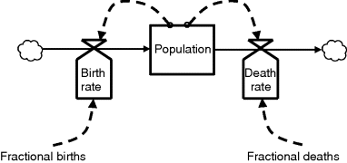
Figure 15.2 Level-rate diagram for simple population dynamics.
Likewise in discrete-event simulation, the pioneers were aware of the power of graphical representation and devised ways to exploit this. The GPSS listing shown earlier actually corresponds to a block diagram in which each line of code is a separate block using some of the symbols shown in Ståhl et al. (2011, Figure 2). The GPSS simulation modeller, probably not an expert programmer, was encouraged to draw a block diagram to represent the system logic and from it to write GPSS code. Each block corresponded to a punched card which formed the program and data entry mechanism for most computers at the time. In the UK, Tocher (1962) uses what were termed stochastic gearwheels, to represent logical interactions between classes of simulation objects. These later evolved into the familiar activity cycle diagrams shown in Chapters 2 and 6.
As computers grew cheaper and more powerful, software developers exploited this and users soon took it for granted that they could interact graphically with simulation software. Thus the now familiar software packages appeared. Stella (isee systems, 2013) was the first widely used graphical system dynamics simulation system and exploited the superior graphics of Apple computers. Stella was followed by Vensim (see Chapter 11) and Powersim (Powersim Corporation, 2013). All three of these provide a graphics palette that allows on-screen model development by drawing diagrams based on Forrester's level-rate graphics. The discrete-event simulation field similarly realised the potential of computer graphics and experienced much more explosive growth than system dynamics. Many different graphical packages appeared, of which well-known examples include SIMUL8 (see Chapter 10), Witness (Lanner, 2013), Arena (Rockwell Automation, 2013) and Simio (Simio, 2013). In addition, various vendors developed graphical software that supports both system dynamics and discrete-event simulation. Examples include AnyLogic (see Chapter 12), which also supports agent-based modelling, and ExtendSim (ImagineThat, 2013).
15.4 The Importance of Process
There is, though, one major difference in the evolution of support for model development and representation for system dynamics and discrete event simulation. The system dynamics community was quicker to recognise that communication with model users and clients was crucial and started to use a different type of influence diagram as a precursor to level-rate schemes and DYNAMO equations. Examples of these influence diagrams are shown in Chapter 6, 11 and 13. Rather than attempting to distinguish between levels (or stocks) and flows (or rates), the aim is simply to represent how one variable might affect another. By doing so, the aim is to understand the feedback behaviour generated by the structure of the system being modelled, which may mean that there is no need actually to develop and run a fully fledged simulation model. Thus the approach described in Wolstenholme (1990), and called qualitative system dynamics in Chapter 6, was born.
This qualitative representation of system structure allowed writers such as Senge (1990) to popularise the idea of system archetypes, enabling the use of qualitative system dynamics in system design as well as analysis.
This brought system dynamics to the attention of the much less technical management learning community, whereas the technical demands of discrete-event simulation meant that, despite its power, its use was mainly restricted to technically trained analysts. In Chapter 10, Mark Elder sensibly argues that such analysts must also pay great attention to the process aspects of their work, using tools like SIMUL8, of which he was originator.
System dynamics and discrete-event simulation have followed similar tracks that were influenced mainly by developments in computing. In addition, system dynamics modellers were quick to realise the power of graphical conceptualisation in influence diagrams. In recent years, both communities have realised that close user engagement in conceptualisation and model development is key to successful implementation of analysis based on simulation modelling.
15.5 My Own Comparison of the Simulation Approaches
The comparisons in the previous chapters are at a conceptual level, but it is helpful, I think, to go into more detail about both system dynamics and discrete-event simulation – to look under the hood. Doing so should help our understanding of why the close integration of the two approaches, if we take them to be simulation methods, may or may not be wise.
15.5.1 Time Handling
The types of system usually simulated by both system dynamics and discrete-event simulation are dynamic, rather than static. That is, things happen through time and the simulation model is intended to capture the effects of those changes, so as to understand why they occur and may be used to investigate what might be done to improve things. A very early definition of computer simulation captures this rather well: ‘Simulation always involves the manipulation of a model so that it yields a motion picture of reality’ (Ackoff and Sasieni, 1968, p. 97). Simulation models run on digital computers, which means, fundamentally, that the progress of time is not smooth, but proceeds in discrete steps. System dynamics and discrete-event simulation models treat this advance in simulated time in different ways. Pidd (2004, Chapter 2) provides examples to illustrate these differences.
As normally implemented, system dynamics simulations employ a time slicing approach in which the system is indexed through simulation time in predefined time increments. These time slices are usually known as dt or DT, depending on the software in use. Thus level (equation 15.1) shown earlier in this chapter includes a constant DT, which represents this time slice. The level equations are updated at these regular intervals to capture the effect of the inflows and outflows over that interval. Once these level equations have been computed, the rate equations are computed to determine the rates that will apply over the next time interval of length DT. A system dynamics model that employs time slicing is actually performing an Euler–Cauchy integration of the difference equations, though this is rarely mentioned in practice. Time slicing is very simple to implement in simulation software and is easily understood.
Most discrete-event simulations model the movement of time rather differently. Instead of employing fixed time slices that are determined in advance, the simulation proceeds from event to event and the intervals between those events vary. Events are state changes that affect one or more entities in the system being simulated. Examples might be the arrival of a patient at an Emergency Department, the discharge of a patient from hospital or the start or finish of a lunch break. To move simulated time from event to event in this way requires a more complex computer program than needed for time slicing, though it is not too difficult to implement. The efficiency of a discrete-event simulation system is to a large extent dependent on the way that its executive is implemented. The executive maintains an event calendar on which future events are entered. At each event time, the executive checks the calendar to see when the next event is due and moves the simulation clock to that time, at which more future events may be entered on the calendar (see Pidd, 2004, Chapter 6, for more details). The intervals between events depend entirely on the rules coded into the entity definitions and will vary. Thus the simulation proceeds quickly when events are sparse, but slows down when events are frequent. If the nature of the system is such that all events occur at regular intervals (e.g. once each day) then a discrete-event simulation automatically defaults to time slicing.
Any attempt to integrate system dynamics and discrete-event models must cope with these different approaches to time handling in the implementation and execution of a simulation. In essence this means that either both models must briefly cease operation in order to exchange data, or the discrete-event model must schedule some regular, time-sliced events so that interaction can occur with the system dynamics model at those regular events. In the accident and emergency model discussed in Chapter 13, the system dynamics and discrete-event models are both stopped every simulated hour to enable this data exchange. A similar approach is taken in the chlamydia integrated model discussed in Chapter 14. The AnyLogic software, which allows system dynamics, discrete-event models and agent-based approaches, manages its integration by forcing system dynamics time points to become discrete events.
15.5.2 Stochastic and Deterministic Elements
Many dynamic systems include non-deterministic elements. Thus we may not be sure exactly how many patients will arrive at an Emergency Department or how long it will take a nurse to treat a patient. These are examples of stochastic elements, a term used to denote something that varies probabilistically through time. Stochastic elements are usually represented in a simulation model by appropriate probability distributions. These may be mathematically defined distributions such as Normal, Poisson and gamma or may be histograms directly based on data. Simulations with stochastic elements employ sampling routines in which random numbers are used to generate samples from the distributions (see Pidd, 2004, Chapter 10, for details).
Discrete-event simulations are usually employed on systems with stochastic elements, whereas most system dynamics models are wholly deterministic. The use of random sampling in a discrete-event simulation means that each simulation run is, in effect, a sampling experiment and each such run will produce different results. How different they are will depend on the extent of the stochastic variation in the model. To allow for this sampling variation, discrete-event modellers employ careful analysis methods to ensure that any conclusions drawn from a set of simulation runs are statistically sound (see Pidd, 2004, Chapter 11, for details). This stochastic variation means that it is usually unwise to draw conclusions based on a single run of a discrete-event simulation.
By contrast, system dynamics models are based on an assumption that system structure leads to system behaviour and that any observed variation in that behaviour is a result of interactions between system substructures. Thus, there is no need to run a system dynamics model many times, unless the values assigned to system parameters vary. For example, in Figure 15.2 we may be uncertain of the percentage of deaths expected each year. This is normally handled by running the model several times, each with different values that represent the likely range of variation in that parameter. This obviously needs careful thought if there are multiple parameters with values that are uncertain. Some system dynamics software allows the modeller to specify that the value of a parameter is sampled from a probability distribution, but this provision feels like an added extra.
Fundamentally, then, system dynamics models are deterministic and discrete-event models are usually stochastic. This means that, in addition to the issues caused by their different approaches to time handling, great care needs to be taken in interpreting the results from an integrated model or those from a pair of cooperating models. In essence the two different types of variation can lead to a factorial explosion when attempting to understand the results of such simulations. As yet, there is no sign that this is an issue to which researchers have given much attention.
15.5.3 Discrete Entities versus Continuous Variables
The basic building blocks of the two approaches also differ. In a discrete-event simulation, the concept of a simulation entity is fundamental. A simulation entity is an object that is included in the simulation model because it changes state and is believed to contribute to the behaviour of the system. Examples might include doctors, nurses and patients in a healthcare simulation or equipment such as imaging machines. The behaviour of some of the entities included in a discrete-event model is likely to be stochastic, which means that the events scheduled for their state changes will not occur at regular, time-sliced intervals. If a discrete-event simulation includes multiple entities of the same type that need to be separately represented, these are usually organised into classes, for example of patients. The entities included in a class need not be identical, but must have enough similarity to allow general statements to be made about their behaviour. For example, unless arriving in an ambulance, patients register their arrival at the clinic before they are seen by a clinician. Fundamentally, discrete-event models (and agent-based models, too) are atomistic, in that system behaviour is a result of interactions occurring between individual entities and the resources they use while in the system being simulated.
By contrast, the fundamental building blocks of system dynamics models are two types of variable: levels (or stocks) and rates (or flows). Levels are accumulations within the system that will persist even if activity ceases elsewhere in the system. Rates represent the activity within a system and control the levels, like inflows and outflows from a tank of liquid. Rates are constant over a time interval DT and levels are computed as a result of those rates at the instants between each time slice. This means that system dynamics variables are quasi-continuous as shown in Figure 15.3, because the rates and levels only change at discrete, predefined points of time and are held constant between the points. That is, a system dynamics model is a quasi-continuous simulation, based on straightforward difference equations in which time moves between discrete, predefined points. The focus of a system dynamics model is the way that the variables vary through simulated time and not on individual items counted within those aggregated variables. Thus system dynamics models are not atomistic, but quasi-continuous aggregations in which variation in behaviour occurs as a result of relationships between the variables included.
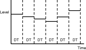
Figure 15.3 Quasi-continuous representation of levels in system dynamics.
As with the differences in time handling and the use of random sampling in a discrete-event model, the emphasis on discrete entities or continuous variables presents issues to be faced when attempting to integrate or cooperate the two approaches. It is relatively straightforward to use the value taken by a continuous variable to fire a discrete event. For example, if the number of patients seen in a clinic reaches some prescribed value, the simulation may ensure that extra staff are drafted in. That is, the value of a continuous variable may affect the population of entities in a discrete-event simulation. Chapter 12, which describes the operation of the AnyLogic simulation software, provides a thorough discussion of the different ways that discrete entities and continuous variables may interact in a simulation that contains both types of object.
We might note in passing that simulation time in a discrete-event simulation is actually a quasi-continuous variable, albeit one that changes its value at non-constant intervals. Since most discrete-event software implements efficient mechanisms for managing this quasi-continuous variable via an event calendar, it is worth speculating on whether a similar approach could be used to manage interactions between a discrete-event simulation and a system dynamics model. This might be a fertile research area to pursue.
15.6 Linking System Dynamics and Discrete-Event Simulation
Any attempt to link system dynamics and discrete-event simulation must take account of their different ways of handling simulated time, their assumptions about the causes of variations in system behaviour and the different degrees of aggregation. None of these is insurmountable, as is evidenced by software such as AnyLogic and ExtendSim, which allow both approaches to coexist within the same model.
Broadly speaking, there are three ways in which the two approaches may be linked and these are summarised in Figure 15.4:
- The close integration of different approaches within a single model: examples of this might be the use of AnyLogic or ExtendSim to embed both discrete-event and system dynamics elements within the same model.
- The loose coupling of different approaches: examples might be situations in which a discrete-event simulation model runs separately from a system dynamics model and the two periodically communicate and exchange data. This is described as parallel interaction in Chapter 13 and as combined modelling in the description of the chlamydia model in Chapter 14.
- The use of one approach as a precursor to the other. For example, values produced from a discrete-event simulation might be used as parameters in a system dynamics model, or vice versa. This is described as sequential interaction in Chapter 13.

Figure 15.4 Ways to combine system dynamics and discrete-event simulation.
Whether it is always wise to have both elements within the same model is another question altogether and asserting that a real-world system contains both continuous and discrete elements may not be cause enough. It is important to remember that models are always simplifications. Pidd (2009, pp. 8–10) defines a model as ‘an external and explicit representation of part of reality as seen by the people who wish to use that model to understand, to change, to manage and to control that part of reality’. The aim of a systems modelling exercise is to find some way to represent the factors that are believed to contribute to the aspects of the behaviour of the system in which we are interested. That is, choices have to be made and some factors will be included and others excluded. Even if a factor is included, it may be possible to represent in an approximate way that avoids the need to operate a combined model.
This book does not include a detailed discussion of model validation, but this is an important part of any modelling exercise if modellers and model users are to have confidence in the results produced by the model. It may be sufficient to represent continuous variables by discrete elements and build a wholly discrete-event simulation. Alternatively, it may be sufficient to represent discrete elements by suitable equation parameters in a system dynamics model. No modelling exercise is perfect and no model is 100% accurate. Models need to be fit for purpose and clarity about that purpose is vital. Thus embedding both system dynamics and discrete-event elements in a model is possible, but may not be necessary – depending on the intended use of the model.
15.7 The Importance of Intended Model Use
Though there is never a guarantee that a model will be used for its intended purpose, or indeed whether it will ever be used at all, the intended model use should always be a major determinant of what is included in the model and how it is represented. Pidd (2009, p. 66) discusses model use and includes the figure shown simplified here as Figure 15.5. This is a spectrum of model use that includes the four points discussed below. The first two positions (decision automation and routine decision support) are shown as requiring tools for routine decision making. The other two (system investigation and providing insight) are shown as requiring tools for thinking. Clearly these four points are archetypes and in-between positions are possible.

Figure 15.5 A spectrum of model use.
15.7.1 Decision Automation
As used here, the term decision automation refers to situations in which a model is developed to replace routine, human decision making. Many of us use such models regularly but are unaware of it. For example, hotel rooms and airline tickets are sold through web sites, behind which sit one or more automated systems of revenue management. The aim of revenue management systems is to ensure that seats and hotel rooms are offered at prices that are neither too high nor too low. If prices are too high, seats and rooms will be left empty and profit forgone; if they are too low, revenue will be depressed. Revenue management systems rely on automated forecasting models to predict sales at different prices, which cooperate with optimisation models that allocate seats and rooms to price bands through time. From time to time, the parameters of the models will need to be updated to reflect changes that occur in the environment in which the models are employed, but day-to-day routine use is fully automatic.
For successful decision automation, great attention must be paid to model and data accuracy and to speed and efficiency of execution, and it is usually crucial that the model is properly linked to other corporate systems. Since an organisation is trusting the model to take decisions on its behalf and to commit resources, fidelity and detail are crucial, which means that model testing and validation loom large and may require considerable time and resources.
It would, I believe, be most unwise to use either system dynamics or discrete-event simulation, unless the model is wholly deterministic, in a fully automated decision-making process. Once a discrete-event simulation includes stochastic elements, the results of the simulation will vary from run to run, depending on the random sampling processes employed.
This induced variation means that human intervention is needed to interpret the results of the simulation. It would also be unwise to build an automated decision-making system around a system dynamics model because such models are approximate and very aggregated representations that are unlikely to be fine grained enough for routine decision making. Both system dynamics and discrete-event models are best regarded as adjuncts to human decision making.
15.7.2 Routine Decision Support
Models that underpin routine decision support are also used regularly, though less frequently, than those employed in decision automation. The aim here is not to replace human decision makers but to support them. Ensuring that they have the right crews and aircraft in the right place at the right time is a major concern for airlines. Commercial aircraft are very expensive and do not make money when on the ground, so need to be flying full of passengers as often as possible. This requires the correct number of flight crew to be available as well as having the aircraft ready. Having enough aircraft and crew available is easy if the airline employs an excessive number of both, but doing so costs money. Hence the need to get the levels right, which is a complex problem for airlines that operate many flights from many airports.
Considerable effort has gone into developing models to support human decision makers as they plan rosters and schedules, and the accuracy and validity of the models improve each year. However, the models are not used to make decisions, but rather to propose rosters and schedules that a human decision maker can alter because of circumstances of which he or she is aware that are not part of the model. Without the model, the decision maker would face a daunting task of developing rosters and schedules from scratch and is likely to rely on heuristic approaches that may or may not be valid. With a decision support model, the decision maker can greatly reduce his or her work and focus on the areas of uncertainty.
Though, as with models intended for use in decision automation, fidelity and detail are important, there is no requirement for the model to be wholly complete, though this does not mean that sloppy modelling is allowed. Rather, because the model is an adjunct to decision making by humans, there is a recognition that the model and human decision maker working together form the decision-making system. Since the model is to be used regularly, ease of use looms large and there may also be a requirement that it can interface with corporate systems.
Both discrete-event and system dynamics models could be used in routine decision support; however, there are few, if any, reports of their actual use in this way. This may be because discrete-event models are not transparent to the user and because the nature of the results from system dynamics models can seem rather imprecise. Perhaps this may be another fertile area of research for the future?
15.7.3 System Investigation and Improvement
This type of model use is perhaps the most common way in which both system dynamics and discrete-event simulations are employed, particularly the latter. Typically, an organisation or individual wishes to gain better understanding of how a system operates, or to find better ways for it to do so. In the latter case, the model becomes a vehicle for experimentation; an artificial world in which options can be compared and explored before any real implementation. Most simulation case studies reported at conferences or in journals are examples of such work. In this book, most of the examples in the preceding chapters discuss the development and use of discrete-event, system dynamics, linked or hybrid models for such system investigation and improvement.
Earlier in this chapter I argued that system dynamics modellers realised the importance of the process of interactive model building much earlier than did their discrete-event counterparts. When seeking system improvement a triad of modeller, decision maker and model constitute the decision-making, or learning, system. Indeed, when a model is developed for use in system investigation and improvement, the processes of model conceptualisation, development and validation become a learning process for all involved. It is sometimes the case that creating the model provides enough insights for people to act with confidence without actually running the model. In this regard, visualisation, whether paper-based or on-screen, becomes very important, to help participants strive for common understanding of the system being simulated.
Given all this, it should be no surprise that both discrete-event and system dynamics approaches can be used, and are used, to develop models to support system investigation and improvement. Indeed, most books on these subjects assume that this is why the model is to be developed.
15.7.4 Providing Insights for Debate
The final point on the spectrum of Figure 15.5 is labelled as providing insights for debate. Whereas decision automation may be appropriate for operational decisions, here we are concerned with strategy and policy issues in which people may hold fundamentally different positions. Strategic decisions are rarely made solely on the basis of the results from running a simulation model and this is especially true in public policy, as discussed in Thissen and Walker (2013). Instead, people argue their case and it can be helpful to understand and demonstrate the effect of their beliefs about how a system does or might operate. There is an underlying assumption in the other three positions that the model is representing something ‘out there’, but models developed to provide insights for debate are more often concerned with explicating mental models.
The explication of mental models has long been a concern in the system dynamics community. As pointed out by Doyle and Ford (1998), mental models were a major concern of the Industrial Dynamics book (Forrester, 1961), and Forrester (1971) elaborates further on this theme. Forrester's main argument is that everyone has mental models of how systems operate or could operate and the job of a modeller is to tease these out and to represent them explicitly. Once explicated, they are available for clear discussion and debate.
Thissen and Walker (2013) argue that rational analysis has a place in public policy development and suggest that this explication is an important contribution from the analytical community. However, it should be noted that the political arena is characterised by ambiguity and sometime this is essential if accommodation is to be achieved between warring parties (Noordegraaf and Abma, 2003). This does not mean that modelling has no place in policy analysis, but it does suggest that its use may require political skill and a willingness to live with ambiguity rather than to insist on its removal.
Although discrete-event simulations could be used in policy debate, they are more often used later, after agreement has been reached about the broad shape of a policy that now needs tuning. By contrast, system dynamics is an approach that could be used to support some types of policy development, particularly for the exploration of scenarios, in which ambiguity plays an important role.
15.8 The Future?
Attempting to forecast the future more than a short period ahead is a risky business. It was, after all, Thomas Watson, Chairman of IBM, who stated in 1943 that the world market for computers would be no more than five. One of the lessons of longer term business forecasting is that flexible responses to changes in the environment may be more important than apparent forecasting accuracy. Hence, in this final section I will attempt to examine what might happen to system dynamics and discrete-event simulation in the future. Inevitably, this exploration is based on my own prejudices and experience, as well as evidence from the past.
15.8.1 Use of Both Methods will Continue to Grow
Figure 15.1 gives some idea of the growth in the use of both approaches over the last 30 years. What might cause such growth to stall or to be reversed? Two possibilities come to mind. The first is that better and more appropriate methods might appear and become popular. Perhaps Keith Tocher was right and developments in mathematical statistics will mean it is unnecessary to use discrete-event simulation? It is very likely that new methods will be developed and used that will make the use of simulation unnecessary in some projects. However, little has happened in the last 50 years that makes such a major decline very likely, so it seems that the need for discrete-event simulation will remain. System dynamics likewise offers an appealingly simple formalism for thinking about the behaviour of dynamic systems.
For both approaches, new or expanding application areas have appeared and will continue to do so. For example, though discrete-event simulation has been used in healthcare for many years (Tunnicliffe-Wilson, 1981) its use has grown greatly in recent years. For example, the 2000 Winter Simulation Conference, which has a main focus on discrete-event simulation, had only a partial stream of seven papers devoted to healthcare. In 2006, the conference introduced a full Healthcare track, which included nine papers. By 2012 this track had grown to 32 papers. It is harder to establish the similar growth in system dynamics, as the organisation of the Proceedings of the International Conferences of the System Dynamics Society is harder to disentangle in its earlier years; however, the other chapters of this book suggest that this is currently a major area of activity. Why has this growth occurred? Because healthcare is expensive and there is a need to increase its efficiency and effectiveness and both system dynamics and discrete-event simulation are a great help in this. At some point, growth in modelling work in healthcare will slow down and may even decline, but it seems likely that new application areas will appear because they face similar issues and require the use of similar approaches.
15.8.2 Developments in Computing will Continue to have an Effect
I argued earlier that much of the previous growth in the use of both approaches was due to developments in computing technology. In the very early years of discrete-event simulation, there was two-way traffic between the worlds of simulation and computing. For example, the basic ideas of object orientation were first implemented in Simula, a much underused simulation programming language. However, in the last 20 years or so simulation software providers have been quick to exploit developments in computing and it seems likely that this trend will continue. What none of us know is what these developments will be, but the following few seem likely.
Most users now take mobile computing for granted and today's smartphones are much more powerful than the PCs of a decade ago. Smartphones and tablet computers have more than enough power to run simulations, especially if parts of the execution are managed over the Internet. This cooperative execution has been possible for some time with Web-based SIMUL8 (SIMUL8 Corporation, 2013), which allows a user to run part of the simulation on a PC and with the rest run on a Web-based, or intranet, server. There is no technical reason why simulations, whether system dynamics or discrete-event, cannot be run on a smartphone or tablet or via a Web-based cooperation. This does not mean, however, that such devices are ideal for model development, in which small screen size is a definite handicap.
For model development, especially when this is group-based, it seems obvious that the two communities should exploit large graphics walls with touch-based interfaces. In 2013, when I wrote this chapter, I visited my three-year-old granddaughter's nursery and saw that she and her playmates knew how to use a smart-board. Better large display walls could enable group participation, allowing people to stand and create models on-the-fly, assuming the software is smart enough to exploit this. Since 1987, the advocates of the Strategic Choice Approach (Friend and Hickling, 1987) have argued that allowing people to walk around and to stand while considering strategic options adds greatly to the value of strategic discussions. Large display walls with touch-based interfaces running simulation software would seem to be ideal for this.
Ubiquitous computing is now ubiquitous. That is, we take for granted that the devices that we use in our mundane, daily lives are smart, and this is because they include embedded computing devices. The defence community has long been a user of ‘man in the loop’ simulations in which humans interact with computer simulations, sometimes for training, but also in strategy and tactical development. These approaches recognise that it is better to allow humans really to interact than to try to model those interactions. It seems possible that wearable or implantable computing devices may be of great value in further developing these approaches.
15.8.3 Process Really Matters
Earlier in this chapter, I argued that the system dynamics community was quick to realise that much modelling involves the explication of mental models, which requires careful process management. This emphasis continues to this day. The discrete-event simulation community came rather later to the same view, partly because its models are usually rather more complex than system dynamics models. Thus, part of Mark Elder's argument in Chapter 10 is that highly developed skills in computing and statistics are no guarantee that a modeller will be effective in helping users to employ simulation so as to develop and understand options for change. This also chimes with the recent emphasis on conceptual modelling (Robinson et al., 2011) in discrete-event simulation, which stresses that conceptualisation is a process rather than an outcome. Likewise, it also links into the theme developed in Chapter 4 by Kathy Kotiadis and John Mingers that problem structuring methods can and should be combined with simulation approaches, though this needs to be done with some care. This emphasis on carefully managed processes for model use and development also seems set to continue and we may expect the appearance of further tools to support this.
References
- Ackoff, R.L. and Sasieni, M.W. (1968) Fundamentals of Operations Research, John Wiley & Sons, Inc., New York.
- Doyle, J.K. and Ford, D.N. (1998) Mental models concepts for system dynamics research. System Dynamics Review, 14, (Spring), 1.
- Forrester, J.W. (1958) Industrial dynamics: a major breakthrough for decision makers. Harvard Business Review, 36 (4), 37–66.
- Forrester, J.W. (1961) Industrial Dynamics, MIT Press, Cambridge, MA.
- Forrester, J.W. (1971) Counterintuitive behavior of social systems, in Collected Papers of J. W. Forrester, Wright-Allen Press, Cambridge, MA, pp. 211–244.
- Friend, J.K. and Hickling, A. (1987) Planning Under Pressure: The Strategic Choice Approach, Pergamon Press, Oxford.
- Gordon, G. (1962) A general purpose system simulator. IBM Systems Journal, 1, 18–32.
- Hollocks, B.W. (2006) Forty years of discrete-event simulation: a personal reflection. Journal of the Operational Research Society, 57 (12), 1383–1399.
- ImagineThat (2013) ExtendSim powertools for simulation, www.extendsim.com.
- isee systems (2013) Stella: systems thinking for education and research, www.iseesystems.com.
- Lanner (2013) Witness 12 – Making it easier to provide answers for business critical problems, www.lanner.com.
- Nance, R.E. (1993) A history of discrete event simulation programming languages. Technical Report TR-93-21, Computer Science, Virginia Polytechnic Institute and State University.
- Noordegraaf, M. and Abma, T. (2003) Management by measurement? Public management practices amidst ambiguity. Public Administration, 81 (4), 853–873.
- Pidd, M. (1984) Computer Simulation in Management Science, 1st edn., John Wiley & Sons, Ltd, Chichester.
- Pidd, M. (2004) Computer Simulation in Management Science, 5th edn., John Wiley & Sons, Ltd, Chichester.
- Pidd, M. (2009) Tools for Thinking: Modelling in Management Science, 3rd edn., John Wiley & Sons, Ltd, Chichester.
- Powersim Corporation (2013) Powersim, www.powersim.com.
- Pugh, A.L. (1973) DYNAMO II User's Manual, MIT Press, Cambridge, MA.
- Robinson, S.L., Brooks, R., Kotiadis, K. and van der Zee, D.-.K. (eds) (2011) Conceptual Modelling for Discrete-Event Simulation, CRC Press, Boca Raton, FL.
- Rockwell Automation (2013) Arena simulation software, www.arenasimulation.com.
- Senge, P.M. (1990) The Fifth Disciple: The Art and Practice of the Learning Organization, Random House, London.
- Simio (2013) Simio simulation software, www.simio.com.
- SIMUL8 Corporation (2013) Web based SIMUL8, www.simul8.com/products/simul8_web.htm.
- Ståhl, I., Henricksen, J.O., Born, R.G. and Herper, H. (2011) GPSS 50 years old, but still young. Proceedings of the 2011 Winter Simulation Conference, Phoenix, AZ.
- Thissen, W.A.H. and Walker, W.E. (eds) (2013) Public Policy Analysis: New Developments, International Series in Operations Research & Management Science, vol. 179, Springer, New York.
- Tocher, K.D. (1962) The Art of Simulation, English Universities Press, London.
- Tunnicliffe Wilson, J.C. (1981) Implementation of computer simulation projects in health care. Journal of the Operational Research Society, 32, 825–832.
- Wolstenholme, E.F. (1990) System Enquiry: A System Dynamics Approach, John Wiley & Sons, Ltd, Chichester.