8. Three-Phase Transformer Models

Search in book...
Toggle Font Controls
Create new playlist

Name your new playlist

Playlist description (optional)
Sign In

Email address

Password

Forgot Password?

or

Continue with Facebook

Continue with Google
Sign Up

Full Name

Email address

Confirm Email Address

Password

or

Continue with Facebook

Continue with Google

Three-phase transformer banks are found in the distribution substation, where the voltage is transformed from the transmission or subtransmission level to the distribution feeder level. In most cases, the substation transformer will be a three-phase unit, perhaps with high-voltage no-load taps and, perhaps, low-voltage load tap changing (LTC). For a four-wire wye feeder, the most common substation transformer connection is the delta–grounded wye. A three-wire delta feeder will typically have a delta–delta transformer connection in the substation. Three-phase transformer banks downstream from the substation will provide the final voltage transformation to the customer’s load. A variety of transformer connections can be applied. The load can be pure three-phase or a combination of single-phase lighting load and a three-phase load such as an induction motor. In the analysis of a distribution feeder, it is important that the various three-phase transformer connections be modeled correctly.

Unique models of three-phase transformer banks applicable to radial distribution feeders will be developed in this chapter. Models for the following three-phase connections are included:

Delta–grounded wye
Ungrounded wye–delta
Grounded wye–delta
Open wye–open delta
Grounded wye–grounded wye
Delta–delta
Open delta–open delta

8.1 Introduction

Figure 8.1 defines the various voltages and currents for all three-phase transformer banks connected between the source-side node n and the load-side node m.

images

Figure 8.1
General three-phase transformer bank.

In Figure 8.1, the models can represent a step-down (source side to load side) or a step-up (source side to load side) transformer bank. The notation is such that the capital letters A, B, C, and N will always refer to the source side (node n) of the bank, and the lower case letters a, b, c, and n will always refer to the load side (node m) of the bank. It is assumed that all variations of the wye–delta connections are connected in the “American Standard Thirty Degree” connection. The described phase notation and the standard phase shifts for positive sequence voltages and currents are:

Step-down connection

$V_{A B} leads V_{a b} {by 30}^{\circ}$ (8.1)

$I_{A} leads I_{a} {by 30}^{\circ}$ (8.2)

Step-up connection

$V_{a b} leads V_{A B} {by 30}^{\circ}$ (8.3)

$I_{a} leads I_{A} {by 30}^{\circ}$ (8.4)

8.2 Generalized Matrices

The models to be used in power-flow and short-circuit studies are generalized for the connections in the same form as have been developed for line segments (Chapter 6) and voltage regulators (Chapter 7). In the “forward sweep” of the “ladder” iterative technique described in Chapter 10, the voltages at node m are defined as a function of the voltages at node n and the currents at node m. The required equation is:

$[V_{L N_{a b c}}] = [A_{t}] \cdot [V_{L N_{A B C}}] - [B_{t}] \cdot [I_{a b c}]$ (8.5)

In the “backward sweep” of the ladder technique, the matrix equations for computing the voltages and currents at node n as a function of the voltages and currents at node m are given by:

$[V_{L N_{A B C}}] = [a_{t}] \cdot [V_{L N_{a b c}}] + [b_{t}] \cdot [I_{a b c}]$ (8.6)

$[I_{A B C}] = [c_{t}] \cdot [V_{L N_{a b c}}] + [d_{t}] \cdot [I_{a b c}]$ (8.7)

In Equations 8.5, 8.6, and 8.7, the matrices [VLN_ABC] and [VLN_abc] represent the line-to-neutral voltages for an ungrounded wye connection or the line-to-ground voltages for a grounded wye connection. For a delta connection, the voltage matrices represent “equivalent” line-to-neutral voltages. The current matrices represent the line currents regardless of the transformer winding connection.

In the modified ladder technique, Equation 8.5 is used to compute new node voltages downstream from the source using the most recent line currents. In the backward sweep, only Equation 8.7 is used to compute the source-side line currents using the newly computed load-side line currents.

8.3 The Delta–Grounded Wye Step-Down Connection

The delta–grounded wye step-down connection is a popular connection that is typically used in a distribution substation serving a four-wire wye feeder system. Another application of the connection is to provide service to a load that is primarily single-phase. Because of the wye connection, three single-phase circuits are available, thereby making it possible to balance the single-phase loading on the transformer bank.

Three single-phase transformers can be connected delta–grounded wye in a “standard 30° step-down connection” (as shown in Figure 8.2).

8.3.1 Voltages

images

Figure 8.2
Standard delta–grounded wye connection with voltages.

The positive sequence phasor diagrams of the voltages (Figure 8.2) show the relationships between the various positive sequence voltages. Note that the primary line-to-line voltage from A to B leads the secondary line-to-line voltage from a to b by 30°. Care must be taken to observe the polarity marks on the individual transformer windings. In order to simplify the notation, it is necessary to label the “ideal” voltages with voltage polarity markings as shown in Figure 8.2. Observing the polarity markings of the transformer windings, the voltage Vt_a will be 180° out of phase with the voltage V_CA and the voltage Vt_b will be 180° out of phase with the voltage V_AB. Kirchhoff’s Voltage Law at no-load gives the line-to-line voltage between phases a and b as:

$V_{a b} = V_{t}_{_{a}} - V_{t}_{_{b}}$ (8.8)

The phasors of the positive sequence voltages in Equation 8.8 are shown in Figure 8.2.

The magnitude changes between the voltages can be defined in terms of the actual winding turns ratio (n_t). With reference to Figure 8.2, these ratios are defined as follows:

$n_{t} = \frac{k V_{L L_{rated primary}}}{k V_{L N_{rated secondary}}}$ (8.9)

With reference to Figure 8.2, the line-to-line voltages on the primary side of the transformer connection as a function of the ideal secondary-side voltages are given by:

$[\begin{matrix} V_{A B} \\ V_{B C} \\ V_{C A} \end{matrix}] = n_{t} \cdot [\begin{matrix} 0 & - 1 & 0 \\ 0 & 0 & - 1 \\ - 1 & 0 & 0 \end{matrix}] \cdot [\begin{matrix} V_{t}_{_{a}} \\ V_{t}_{_{b}} \\ V_{t}_{_{c}} \end{matrix}] [V_{L L_{A B C}}] = [A V] \cdot [V_{t}_{_{a b c}}]$ (8.10)

where

$[A V] = n_{t} \cdot [\begin{matrix} 0 & - 1 & 0 \\ 0 & 0 & - 1 \\ - 1 & 0 & 0 \end{matrix}]$

Equation 8.10 gives the primary line-to-line voltages at node n as a function of the ideal secondary voltages. However, what is needed is a relationship between “equivalent” line-to-neutral voltages at node n and the ideal secondary voltages. The question is how the equivalent line-to-neutral voltages are determined knowing the line-to-line voltages. One approach is to apply the theory of symmetrical components.

The known line-to-line voltages are transformed to their sequence voltages by:

$[V_{L L_{012}}] = {[A_{s}]}^{- 1} \cdot [V_{L L_{A B C}}]$ (8.11)

where

$[A_{s}] = [\begin{matrix} 1 & 1 & 1 \\ 1 & a_{s}^{2} & a_{s} \\ 1 & a_{s} & a_{s}^{2} \end{matrix}]$ (8.12)

$a_{s} = 1.0 \underset{___}{/ 120}$

By definition, the zero sequence line-to-line voltage is always zero. The relationship between the positive and negative sequence line-to-neutral and line-to-line voltages is known. These relationships in matrix form are given by:

$[\begin{matrix} V_{L N_{0}} \\ V_{L N_{1}} \\ V_{L N_{2}} \end{matrix}] = [\begin{matrix} 1 & 0 & 0 \\ 0 & t_{s}^{*} & 0 \\ 0 & 0 & t_{s} \end{matrix}] \cdot [\begin{matrix} V_{L L_{0}} \\ V_{L L_{1}} \\ V_{L L_{2}} \end{matrix}] [V_{L N_{012}}] = [T] \cdot [V_{L L_{012}}]$ (8.13)

where

$t = \frac{1}{\sqrt{3}} \underset{___}{/ 30}$

Because the zero sequence line-to-line voltage is zero, the (1,1) term of the matrix [T] can be of any value. For the purposes here, the (1,1) term is chosen to have a value of 1.0. Knowing the sequence line-to-neutral voltages, the equivalent line-to-neutral voltages can be determined.

The equivalent line-to-neutral voltages as a function of the sequence line-to-neutral voltages are:

$[V_{L N_{A B C}}] = [A_{s}] \cdot [T] \cdot [V_{L N_{012}}]$ (8.14)

Substitute Equation 8.13 into Equation 8.14:

$[V_{L N_{A B C}}] = [A_{s}] \cdot [T] \cdot [V_{L L_{012}}]$ (8.15)

Substitute Equation 8.11 into Equation 8.15:

$[V_{L N_{A B C}}] = [W] \cdot [V_{L L_{A B C}}]$ (8.16)

where

$[W] = [A_{s}] \cdot [T] \cdot {[A_{s}]}^{- 1} = \frac{1}{3} \cdot [\begin{matrix} 2 & 1 & 0 \\ 0 & 2 & 1 \\ 1 & 0 & 2 \end{matrix}]$ (8.17)

Equation 8.17 provides a method of computing equivalent line-to-neutral voltages from a knowledge of the line-to-line voltages. This is an important relationship that will be used in a variety of ways as other three-phase transformer connections are studied.

To continue on, Equation 8.16 can be substituted into Equation 8.10:

$[V_{L N_{A B C}}] = [W] \cdot [V_{L L}] = [W] \cdot [A V] \cdot [V_{t}_{_{a b c}}] = [a_{t}] \cdot [V_{t}_{_{a b c}}]$ (8.18)

where

$[a_{t}] = [W] \cdot [A V] = \frac{- n_{t}}{3} \cdot [\begin{matrix} 0 & 2 & 1 \\ 1 & 0 & 2 \\ 2 & 1 & 0 \end{matrix}]$ (8.19)

Equation 8.19 defines the generalized [a_t] matrix for the delta–grounded wye step-down connection.

The ideal secondary voltages as a function of the secondary line-to-ground voltages and the secondary line currents are:

$[V_{t}_{_{a b c}}] = [V_{L G_{a b c}}] + [Z_{t}_{_{a b c}}] \cdot [I_{a b c}]$ (8.20)

where

$[Z_{t}_{_{a b c}}] = [\begin{matrix} Z_{t}_{_{a}} & 0 & 0 \\ 0 & Z_{t}_{_{b}} & 0 \\ 0 & 0 & Z_{t}_{_{c}} \end{matrix}]$ (8.21)

Notice in Equation 8.21 that there is no restriction that the impedances of the three transformers be equal.

Substitute Equation 8.20 into Equation 8.18:

$\begin{array}{l} [V_{L N_{A B C}}] = [a_{t}] \cdot ([V_{L G_{a b c}}] + [Z_{t}_{_{a b c}}] \cdot [I_{a b c}]) \\ [V_{L N_{A B C}}] = [a_{t}] \cdot [V_{L G_{a b c}}] + [b_{t}] \cdot [I_{a b c}] \end{array}$ (8.22)

where

$[b_{t}] = [a_{t}] \cdot [Z_{t}_{_{a b c}}] = \frac{- n_{t}}{3} \cdot [\begin{matrix} 0 & 2 \cdot Z_{t}_{_{b}} & Z_{t}_{_{c}} \\ Z_{t}_{_{a}} & 0 & 2 \cdot Z_{t}_{_{c}} \\ 2 \cdot Z_{t}_{_{a}} & Z_{t}_{_{b}} & 0 \end{matrix}]$ (8.23)

The generalized matrices [a_t] and [b_t] have now been defined. The derivation of the generalized matrices [A_t] and [B_t] begins with solving Equation 8.10 for the ideal secondary voltages:

$[V_{t}_{_{a b c}}] = {[A V]}^{- 1} \cdot [V_{L L_{A B C}}]$ (8.24)

The line-to-line voltages as a function of the equivalent line-to-neutral voltages are:

$[V_{L L_{A B C}}] = [D v] \cdot [V_{L N_{A B C}}]$ (8.25)

where

$[D v] = [\begin{matrix} 1 & - 1 & 0 \\ 0 & 1 & - 1 \\ - 1 & 0 & 1 \end{matrix}]$ (8.26)

Substitute Equation 8.25 into Equation 8.24:

$[V_{t}_{_{a b c}}] = {[A V]}^{- 1} \cdot [D v] \cdot [V_{L N_{A B C}}] = [A_{t}] \cdot [V_{L N_{A B C}}]$ (8.27)

where

$[A_{t}] = {[A V]}^{- 1} \cdot [D v] = \frac{1}{n_{t}} \cdot [\begin{matrix} 1 & 0 & - 1 \\ - 1 & 1 & 0 \\ 0 & - 1 & 1 \end{matrix}]$ (8.28)

Substitute Equation 8.20 into Equation 8.27:

$[V_{L G_{a b c}}] + [Z_{t}_{_{a b c}}] \cdot [I_{a b c}] = [A_{t}] \cdot [V_{L N_{A B C}}]$ (8.29)

Rearrange Equation 8.29:

$[V_{L G_{a b c}}] = [A_{t}] \cdot [V_{L N_{A B C}}] - [B_{t}] \cdot [I_{a b c}]$ (8.30)

where

$[B_{t}] = [Z_{t}_{_{a b c}}] = [\begin{matrix} Z_{t}_{_{a}} & 0 & 0 \\ 0 & Z_{t}_{_{b}} & 0 \\ 0 & 0 & Z_{t}_{_{c}} \end{matrix}]$ (8.31)

Equation 8.22 is referred to as the “backward sweep voltage equation,” and Equations 8.30 is referred to as the “forward sweep voltage equation.” Equations 8.22 and 8.30 apply only for the step-down delta–grounded wye transformer. Note that these equations are exactly in the same form as those derived in earlier chapters for line segments and step-voltage regulators.

8.3.2 Currents

The 30° connection specifies that the positive sequence current entering the H₁ terminal will lead the positive sequence current leaving the X₁ terminal by 30°. Figure 8.3 shows the same connection as Figure 8.2 but with the currents instead of the voltages displayed.

As with the voltages, the polarity marks on the transformer windings must be observed for the currents. For example, in Figure 8.3 the current I_a is entering the polarity mark on the low-voltage winding; so the current I_AC flowing out of the polarity mark on the high-voltage winding will be in phase with I_a. This relationship is shown in the phasor diagrams for positive sequence currents in Figure 8.3. Note that the primary line current on phase A leads the secondary phase a current by 30°.

images

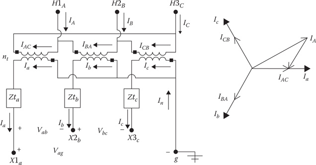
Figure 8.3
Delta–grounded wye connection with currents.

The line currents can be determined as a function of the delta currents by applying Kirchhoff’s Current Law (KCL):

$[\begin{matrix} I_{A} \\ I_{B} \\ I_{C} \end{matrix}] = [\begin{matrix} 1 & - 1 & 0 \\ 0 & 1 & - 1 \\ - 1 & 0 & 1 \end{matrix}] \cdot [\begin{matrix} I_{A C} \\ I_{B A} \\ I_{C B} \end{matrix}]$ (8.32)

In condensed form, Equation 8.32 is:

$[I_{A B C}] = [D] \cdot [I_{D_{A B C}}]$ (8.33)

where

$[D] = [\begin{matrix} 1 & - 1 & 0 \\ 0 & 1 & - 1 \\ - 1 & 0 & 1 \end{matrix}]$

The matrix equation relating the delta primary currents to the secondary line currents is given by:

$[\begin{matrix} I_{A C} \\ I_{B A} \\ I_{C B} \end{matrix}] = \frac{1}{n_{t}} \cdot [\begin{matrix} 1 & 0 & 0 \\ 0 & 1 & 0 \\ 0 & 0 & 1 \end{matrix}] \cdot [\begin{matrix} I_{a} \\ I_{b} \\ I_{c} \end{matrix}]$ (8.34)

$[I_{D}_{_{A B C}}] = [A I] \cdot [I_{a b c}]$ (8.35)

where

$[A I] = \frac{1}{n_{t}} \cdot [\begin{matrix} 1 & 0 & 0 \\ 0 & 1 & 0 \\ 0 & 0 & 1 \end{matrix}]$

Substitute Equation 8.35 into Equation 8.33:

$[I_{A B C}] = [D] \cdot [A I] \cdot [I_{a b c}] = [c_{t}] \cdot [V_{L G_{a b c}}] + [d_{t}] \cdot [I_{a b c}]$ (8.36)

where

$[d_{t}] = [D] \cdot [A I] = \frac{1}{n_{t}} \cdot [\begin{matrix} 1 & - 1 & 0 \\ 0 & 1 & - 1 \\ - 1 & 0 & 1 \end{matrix}]$ (8.37)

$[c_{t}] = [\begin{matrix} 0 & 0 & 0 \\ 0 & 0 & 0 \\ 0 & 0 & 0 \end{matrix}]$ (8.38)

Equation 8.36 (referred to as the “backward sweep current equations”) provides a direct method of computing the phase line currents at node n by knowing the phase line currents at node m. Again, this equation is in the same form as that previously derived for three-phase line segments and three-phase step-voltage regulators.

The equations derived in this section are for the step-down connection. The next section (8.4) will summarize the matrices for the delta–grounded wye step-up connection.

Example 8.1

images

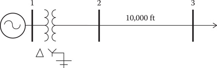
Figure 8.4
Example system.

In the example system in Figure 8.4, an unbalanced constant impedance load is being served at the end of a 10,000-ft section of a three-phase line. The 10,000 ft long line is being fed from a substation transformer rated 5000 kVA, 115 kV delta—12.47 kV grounded wye with a per-unit impedance of 0.085/85. The phase conductors of the line are 336,400 26/7 Aluminum Conductor Steel Reinforced (ACSR) with a neutral conductor 4/0 ACSR. The configuration and computation of the phase impedance matrix are given in Example 4.11. From that example, the phase impedance matrix was computed to be:

$\begin{array}{l} [z_{line}] = [\begin{matrix} 0.4576 + j 1.0780 & 0.1560 + j 0.5017 & 0.1535 + j 0.3849 \\ 0.1560 + j 0.5017 & 0.4666 + j 1.0482 & 0.1580 + j 0.4236 \\ 0.1535 + j 0.3849 & 0.1580 + j 0.4236 & 0.4615 + j 1.0651 \end{matrix}] Ω /mile \\ L = \frac{10, 000}{5280} mile \\ [Z_{{line}_{a b c}}] = L \cdot [z_{line}] = [\begin{matrix} 0.8667 + j 2.0417 & 0.2955 + j 0.9502 & 0.2907 + j 0.7290 \\ 0.2955 + j 0.9502 & 0.8837 + j 1.9852 & 0.2992 + j 0.8023 \\ 0.2907 + j 0.7290 & 0.2992 + j 0.8023 & 0.8741 + j 2.0172 \end{matrix}] \end{array}$

The general matrices for the line are:

$[A_{line}] = [\begin{matrix} 1 & 0 & 0 \\ 0 & 1 & 0 \\ 0 & 0 & 1 \end{matrix}] [B_{line}] = [Z_{{line}_{a b c}}] [d_{line}] = [\begin{matrix} 1 & 0 & 0 \\ 0 & 1 & 0 \\ 0 & 0 & 1 \end{matrix}]$

The transformer impedance needs to be converted to ohms referenced to the low-voltage side of the transformer. The base impedance is:

$Z_{base} = \frac{{12.47}^{2} \cdot 1000}{5000} = 31.1$

The transformer impedance referenced to the low-voltage side is:

$Z_{t} = (0.085 \underset{___}{/ 85}) \cdot 31.3 = 0.2304 + j 2.6335 Ω$

The transformer phase impedance matrix is:

$[Z_{t}_{_{a b c}}] = [\begin{matrix} 0.2304 + j 2.6335 & 0 & 0 \\ 0 & 0.2304 + j 2.6335 & 0 \\ 0 & 0 & 0.2304 + j 2.6335 \end{matrix}] Ω$

The unbalanced constant impedance load is connected in grounded wye. The load impedance matrix is specified to be:

$[Z_{{load}_{a b c}}] = [\begin{matrix} 12 + j 6 & 0 & 0 \\ 0 & 13 + j 4 & 0 \\ 0 & 0 & 14 + j 5 \end{matrix}] Ω$

The unbalanced line-to-line voltages at node 1 serving the substation transformer are given as:

$[V_{L L_{A B C}}] = [\begin{matrix} 115, 000 \underset{___}{/ 0} \\ 116, 500 \underset{___}{/ - 115.5} \\ 123, 538 \underset{___}{/ 121.7} \end{matrix}] V$

a.Determine the generalized matrices for the transformer:The “transformer turn’s” ratio is:

$n_{t} = \frac{k V_{L L_{high}}}{k V_{L N_{low}}} = \frac{115}{12.47 / \sqrt{3}} = 15.9732$

From Equation 8.19:

$[a_{t}] = \frac{- n_{t}}{3} \cdot [\begin{matrix} 0 & 2 & 1 \\ 1 & 0 & 2 \\ 2 & 1 & 0 \end{matrix}] = [\begin{matrix} 0 & - 10.6488 & - 5.3244 \\ - 5.3244 & 0 & - 10.6488 \\ - 10.6488 & - 5.3244 & 0 \end{matrix}]$

From Equation 8.23:

$[b_{t}] = \frac{- n_{t}}{3} \cdot [\begin{matrix} 0 & 2 \cdot Z_{t} & Z_{t} \\ Z_{t} & 0 & 2 \cdot Z_{t} \\ 2 \cdot Z t & Z_{t} & 0 \end{matrix}]$

$[b_{t}] = [\begin{matrix} 0 & - 2.4535 - j 28.0432 & - 1.2267 - j 14.0216 \\ - 1.2267 - j 14.0216 & 0 & - 2.4535 - j 28.0432 \\ - 2.4535 - j 28.0432 & - 1.2267 - j 14.0216 & 0 \end{matrix}]$

From Equation 8.37:

$[d_{t}] = \frac{1}{n_{t}} \cdot [\begin{matrix} 1 & - 1 & 0 \\ 0 & 1 & - 1 \\ - 1 & 0 & 1 \end{matrix}] = [\begin{matrix} 0.0626 & - 0.0626 & 0 \\ 0 & 0.0626 & - 0.0626 \\ - 0.0626 & 0 & 0.0626 \end{matrix}]$

From Equation 8.28:

$[A_{t}] = \frac{1}{n_{t}} \cdot [\begin{matrix} 1 & 0 & - 1 \\ - 1 & 1 & 0 \\ 0 & - 1 & 1 \end{matrix}] = [\begin{matrix} 0.0626 & 0 & - 0.0626 \\ - 0.0626 & 0.0626 & 0 \\ 0 & - 0.0626 & 0.0626 \end{matrix}]$

From Equation 8.31:

$[B_{t}] = [Z_{t}_{_{a b c}}] = [\begin{matrix} 0.2304 + j 2.6335 & 0 & 0 \\ 0 & 0.2304 + j 2.6335 & 0 \\ 0 & 0 & 0.2304 + j 2.6335 \end{matrix}]$

b.Given the line-to-line voltages at node 1, determine the “ideal” transformer voltages:From Equation 8.13:

$[A V] = n_{t} \cdot [\begin{matrix} 0 & - 1 & 0 \\ 0 & 0 & - 1 \\ - 1 & 0 & 0 \end{matrix}] = [\begin{matrix} 0 & - 15.9732 & 0 \\ 0 & 0 & - 15.9732 \\ - 15.9732 & 0 & 0 \end{matrix}]$

$[V_{t}_{_{a b c}}] = {[A V]}^{- 1} \cdot [V_{L L_{A B C}}] = [\begin{matrix} 7734.1 \underset{______}{/ - 58.3} \\ 7199.6 \underset{_____}{/ 180} \\ 7293.5 \underset{_____}{/ 64.5} \end{matrix}] V$

c. Determine the load currents.Since the load is modeled as constant impedances, the system is linear and the analysis can combine all of the impedances (transformer, line, and load) to an equivalent impedance matrix.Kirchhoff’s Voltage Law (KVL) gives:

$[V_{t}_{_{a b c}}] = ([Z_{t}_{_{a b c}}] + [Z_{{line}_{a b c}}] + [Z_{{load}_{a b c}}]) \cdot [I_{a b c}] = [Z_{{eq}_{a b c}}] \cdot [I_{a b c}]$

$[Z_{{eq}_{a b c}}] = [\begin{matrix} 13.0971 + j 10.6751 & 0.2955 + j 0.9502 & 0.2907 + j .7290 \\ 0.2955 + j 0.9502 & 14.1141 + j 8.6187 & 0.2992 + j 0.8023 \\ 0.2907 + j .7290 & 0.2992 + j 0.8023 & 15.1045 + j 9.6507 \end{matrix}] Ω$

The line currents can now be computed as:

$[I_{a b c}] = {[Z_{{total}_{a b c}}]}^{- 1} \cdot [V_{t}_{_{a b c}}] = [\begin{matrix} 471.7 \underline{/} \underset{____}{- 95.1} \\ 456.7 \underset{____}{/ 149.9} \\ 427.3 \underset{___}{/ 33.5} \end{matrix}] A$

d.Determine the line-to-ground voltages at the load in volts and on a 120-V base.

$[V_{{load}_{a b c}}] = [Z_{{load}_{a b c}}] \cdot [I_{a b c}] = [\begin{matrix} 6328.1 \underset{_____}{/ - 68.6} \\ 6212.2 \underset{_____}{/ 167.0} \\ 6352.6 \underset{_____}{/ 53.1} \end{matrix}] V$

The load voltages on a 120-V base are:

$[V_{{load}_{120}}] = [\begin{matrix} 105.5 \underset{_____}{/ - 68.6} \\ 103.5 \underset{_____}{/ 167.0} \\ 105.9 \underset{_____}{/ 53.1} \end{matrix}]$

The line-to-ground voltages at node 2 are:

$[V_{L G_{a b c}}] = [a_{line}] \cdot [V_{{load}_{a b c}}] + [b_{line}] \cdot [I_{a b c}] = [\begin{matrix} 6965.4 \underset{_____}{/ - 66.0} \\ 6580.6 \underset{_____}{/ 171.4} \\ 6691.4 \underset{_____}{/ 56.7} \end{matrix}] V$

e.Using the backward sweep voltage equation, determine the equivalent line-to-neutral voltages and the line-to-line voltages at node 1.

$[V_{L N_{A B C}}] = [a_{t}] \cdot [V_{L G_{a b c}}] + [b_{t}] . [I_{a b c}] = [\begin{matrix} 69.443 \underset{_____}{/ - 30.3} \\ 65, 263 \underset{_____}{/ - 147.5} \\ 70, 272 \underset{_____}{/ 94.0} \end{matrix}] V$

$[V_{L L_{A B C}}] = [D v] \cdot [V_{L N_{A B C}} a] = [\begin{matrix} 115, 000 \underset{__}{/ 0} \\ 116, 500 \underset{_____}{- 115.5} \\ 123.538 \underset{_____}{/ 121.7} \end{matrix}] V$

It is always comforting to be able to work back and compute what was initially given. In this case, the line-to-line voltages at node 1 have been computed, and the same values result that were given at the start of the problem.f.Use the forward sweep voltage equation to verify that the line-to-ground voltages at node 2 can be computed knowing the equivalent line-to-neutral voltages at node 1 and the currents leaving node 2.

$[V_{L G_{a b c}}] = [A_{t}] \cdot [V_{L N_{A B C}}] - [B_{t}] . [I_{a b c}] = [\begin{matrix} 6965.4 \underset{______}{/ - 66.0} \\ 6580.6 \underset{_____}{/ 171.4} \\ 6691.4 \underset{_____}{/ 56.7} \end{matrix}] V$

These are the same values of the line-to-ground voltages at node 2 that were determined working from the load toward the source.

Example 8.1 has demonstrated the application of the forward and backward sweep equations. The example also provides verification that the same voltages and currents result working from the load toward the source or from the source toward the load.

In Example 8.2, the system in Example 8.1 is used only when the source voltages at node 1 are specified and the three-phase load is specified as constant PQ. Because this makes the system nonlinear, the ladder iterative technique must be used to solve for the system voltages and currents.

Example 8.2

Use the system in Example 8.1. The source voltages at node 1 are:

$[E_{L N_{A B C}}] = [\begin{matrix} 115, 000 \underset{__}{/ 0} \\ 115, 000 \underset{_____}{/ - 120} \\ 115, 000 \underset{_____}{/ 120} \end{matrix}]$

The wye-connected loads are:

$[k V A] = [\begin{matrix} 1700 \\ 1200 \\ 1500 \end{matrix}] [P F] = [\begin{matrix} 0.90 \\ 0.85 \\ 0.95 \end{matrix}]$

The complex powers of the loads are computed to be:

$S L_{i} = k V A_{i} \cdot e^{j \cdot a \cos (P F_{i})} = [\begin{matrix} 1530 + j 741.0 \\ 1020 + j 632.1 \\ 1425 + j 468.4 \end{matrix}] kW+ j k v a r$

The ladder iterative technique must be used to analyze the system. A simple Mathcad program is initialized with:

$[I_{start}] = [\begin{matrix} 0 \\ 0 \\ 0 \end{matrix}] Tol = 0.000001 V M = \frac{12, 470}{\sqrt{3}} = 7199.5579 o$

The Mathcad program is shown in Figure 8.5. Note in this routine that in the forward sweep, the secondary transformer voltages are first computed and then those are used to compute the voltages at the loads. At the end of the routine, the newly calculated line currents are taken back to the top of the routine and used to compute the new voltages. This continues until the error in the difference between the two most recently calculated load voltages is less than the tolerance. As a last step, after conversion, the primary currents of the transformer are computed.

images

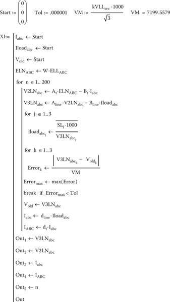
Figure 8.5
Example 8.2 Mathcad program.

After nine iterations, the load voltages and currents are:

$\begin{array}{l} [V_{L N_{load}}] = [\begin{matrix} 6490.1 \underset{_____}{/ - 66.7} \\ 6772.4 \underset{_____}{/ 176.2} \\ 6699.4 \underset{_____}{/ 53.9} \end{matrix}] \\ [I_{a b c}] = [\begin{matrix} 261.9 \underset{_____}{/ - 92.5} \\ 177.2 \underset{_____}{/ 144.4} \\ 223.9 \underset{_____}{/ 35.7} \end{matrix}] \end{array}$

The primary currents are:

$[I_{A B C}] = [\begin{matrix} 24.3 \underset{_____}{/ - 70.0} \\ 20.5 \underset{_____}{/ - 175.2} \\ 27.4 \underset{_____}{/ 63.8} \end{matrix}]$

The magnitude of the load voltages on a 120-V base are:

$[V_{{load}_{120}}] = [\begin{matrix} 108.2 \underset{_____}{/} \underset{_____}{- 66.6} \\ 112.9 \underset{_____}{/ 176.2} \\ 111.7 \underset{_____}{53.9} \end{matrix}]$

Needless to say, these voltages are not acceptable. In order to correct this problem, three step-voltage regulators can be installed at the secondary terminals of the substation transformer as shown in Figure 8.6. The voltage level set on the regulator is 120 V with a bandwidth of 2 V.

Using the method as outlined in Chapter 7, the initial steps for the three regulators are:

$\begin{array}{l} {Tap}_{i} = \frac{| 119 - | V_{{load}_{120_{i}}} | |}{0.75} = [\begin{matrix} 14.44 \\ 8.17 \\ 9.79 \end{matrix}] \\ Round off tap: Tap = [\begin{matrix} 14 \\ 8 \\ 10 \end{matrix}] \end{array}$

With these tap positions, the load voltages are:

$V_{{load}_{120}} = [\begin{matrix} 119.8 \underset{_____}{/ - 66.2} \\ 118.9 \underset{_____}{/ 176.3} \\ 119.7 \underset{_____}{/ 54.1} \end{matrix}] V$

images

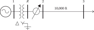
Figure 8.6
Voltage regulators installed.

Because the phase b voltage is low, the phase b tap is changed to 9.

$[Tap] = [\begin{matrix} 14 \\ 9 \\ 10 \end{matrix}]$

The regulator turns ratios are:

$a R_{i} = 1 - .00625 \cdot {Tap}_{i} = [\begin{matrix} 0.9125 \\ 0.9438 \\ 0.9375 \end{matrix}]$

The regulator matrices are:

$\begin{array}{l} [A_{reg}] = [d_{reg}] = [\begin{matrix} \frac{1}{a R_{1}} & 0 & 0 \\ 0 & \frac{1}{a R_{2}} & 0 \\ 0 & 0 & \frac{1}{a R_{3}} \end{matrix}] = [\begin{matrix} 1.0959 & 0 & 0 \\ 0 & 1.0596 & 0 \\ 0 & 0 & 1.0667 \end{matrix}] \\ [B_{reg}] = [\begin{matrix} 0 & 0 & 0 \\ 0 & 0 & 0 \\ 0 & 0 & 0 \end{matrix}] \end{array}$

At the start of the Mathcad routine, the following equation is added:

$I_{reg} \leftarrow Start$

In the Mathcad routine, the first three equations inside the n loop are:

$\begin{array}{l} V_{R_{a b c}} \leftarrow A_{t} \cdot E_{L N_{A B C}} - B_{t} \cdot I_{reg} \\ V_{2 L N_{a b c}} \leftarrow A_{r e g} \cdot V_{{reg}_{a b c}} - B_{reg} \cdot I_{a b c} \\ V_{3 L N_{a b c}} \leftarrow A_{l i n e} \cdot V_{2 L N_{a b c}} - B_{line} \cdot I_{a b c} \end{array}$

At the end of the loop, the following equations are added:

$\begin{array}{l} I_{reg} \leftarrow d_{reg} \cdot I_{a b c} \\ I_{A B C} \leftarrow d_{t} \cdot I_{reg} \end{array}$

With the three regulators installed, the load voltages on a 120-V base are:

$[V_{{load}_{a b c}}] = [\begin{matrix} 119.8 \underset{_____}{/ - 66.2} \\ 119.7 \underset{_____}{/ 176.3} \\ 119.7 \underset{_____}{/ 54.1} \end{matrix}] V$

As can be seen from this example, as more elements of a system are added, there will be one equation for each of the system elements for the forward sweep and backward sweeps. This concept will be further developed in later chapters.

8.4 The Delta–Grounded Wye Step-Up Connection

Figure 8.7 shows the connection diagram for the delta–grounded wye step-up connection.

The no-load phasor diagrams for the voltages and currents are also shown in Figure 8.7. Note that the high-side (primary) line-to-line voltage from A to B lags the low-side (secondary) line-to-line voltage from a to b by 30°, and the same can be said for the high- and low-side line currents.

The development of the generalized matrices follows the same procedure as was used for the step-down connection. Only two matrices differ between the two connections.

The primary (low-side) line-to-line voltages are given by:

$[\begin{matrix} V_{A B} \\ V_{B C} \\ V_{C A} \end{matrix}] = n_{t} \cdot [\begin{matrix} 1 & 0 & 0 \\ 0 & 1 & 0 \\ 0 & 0 & 1 \end{matrix}] \cdot [\begin{matrix} V_{t}_{_{a}} \\ V_{t}_{_{b}} \\ V_{t}_{_{c}} \end{matrix}] [V_{L L_{A B C}}] = [A V] \cdot [V_{t}_{_{a b c}}]$ (8.39)

where

$[A V] = n_{t} \cdot [\begin{matrix} 1 & 0 & 0 \\ 0 & 1 & 0 \\ 0 & 0 & 1 \end{matrix}]$

$n_{t} = \frac{k V_{L L_{rated primary}}}{k V_{L N_{rated secondary}}}$

The primary delta currents are given by:

$[\begin{matrix} I_{A B} \\ I_{B C} \\ I_{C A} \end{matrix}] = \frac{1}{n_{t}} \cdot [\begin{matrix} 1 & 0 & 0 \\ 0 & 1 & 0 \\ 0 & 0 & 1 \end{matrix}] \cdot [\begin{matrix} I_{a} \\ I_{b} \\ I_{c} \end{matrix}] [I_{D_{A B C}}] = [A I] \cdot [I_{a b c}]$ (8.40)

where

$[A I] = \frac{1}{n_{t}} \cdot [\begin{matrix} 1 & 0 & 0 \\ 0 & 1 & 0 \\ 0 & 0 & 1 \end{matrix}]$

images

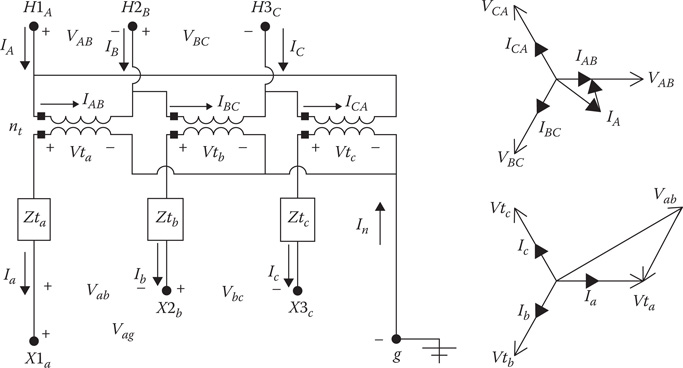
Figure 8.7
Delta–grounded wye step-up connection.

The primary line currents are given by:

$[\begin{matrix} I_{A} \\ I_{B} \\ I_{C} \end{matrix}] = [\begin{matrix} 1 & 0 & - 1 \\ - 1 & 1 & 0 \\ 0 & - 1 & 1 \end{matrix}] \cdot [\begin{matrix} I_{A B} \\ I_{B C} \\ I_{C A} \end{matrix}] [I_{A B C}] = [D i] \cdot [I_{D_{A B C}}]$ (8.41)

where

$[D i] = [\begin{matrix} 1 & 0 & - 1 \\ - 1 & 1 & 0 \\ 0 & - 1 & 1 \end{matrix}]$

The forward sweep matrices are:

Applying Equation 8.28:

$[A_{t}] = A V^{- 1} \cdot D i = \frac{1}{n_{t}} \cdot [\begin{matrix} 1 & 0 & - 1 \\ 0 & 1 & - 1 \\ - 1 & 0 & 1 \end{matrix}]$ (8.42)

Applying Equation 8.31:

$[B_{t}] = [Z_{t}_{_{a b c}}] = [\begin{matrix} Z_{t}_{_{a}} & 0 & 0 \\ 0 & Z_{t}_{_{b}} & 0 \\ 0 & 0 & Z_{t}_{_{c}} \end{matrix}]$ (8.43)

The backward sweep matrices are:

Applying Equation 8.19:

$[a_{t}] = [W] \cdot [A V] = \frac{n_{t}}{3} \cdot [\begin{matrix} 2 & 1 & 0 \\ 0 & 2 & 1 \\ 1 & 0 & 2 \end{matrix}]$ (8.44)

Applying Equation 8.23:

$[b_{t}] = [a_{t}] \cdot [Z_{t}_{_{a b c}}] = \frac{n_{t}}{3} \cdot [\begin{matrix} 2 \cdot Z_{t}_{_{a}} & Z_{t}_{_{b}} & 0 \\ 0 & 2 \cdot Z_{t}_{_{b}} & Z_{t}_{_{c}} \\ Z_{t}_{_{a}} & 0 & 2 \cdot Z_{t}_{_{c}} \end{matrix}]$ (8.45)

Applying Equation 8.37:

$[d_{t}] = [D i] \cdot [A I] = \frac{1}{n_{t}} \cdot [\begin{matrix} 1 & 0 & - 1 \\ 0 & 1 & - 1 \\ - 1 & 0 & 1 \end{matrix}]$ (8.46)

8.5 The Ungrounded Wye–Delta Step-Down Connection

Three single-phase transformers can be connected in a wye–delta connection. The neutral of the wye can be grounded or ungrounded. The grounded wye connection is characterized by the following:

The grounded wye provides a path for zero sequence currents for line-to-ground faults upstream from the transformer bank. This causes the transformers to be susceptible to burnouts on the upstream faults.
If one phase of the primary circuit is opened, the transformer bank will continue to provide three-phase service by operating as an open wye–open delta bank. However, the two remaining transformers may be subject to an overload condition leading to burnout.

The most common connection is the ungrounded wye–delta. This connection is typically used to provide service to a combination of single-phase “lighting” load and a three-phase “power” load such as an induction motor. The generalized constants for the ungrounded wye–delta transformer connection will be developed following the same procedure as was used for the delta–grounded wye.

Three single-phase transformers can be connected in an ungrounded wye “standard 30° step-down connection” as shown in Figure 8.8.

The voltage phasor diagrams in Figure 8.7 illustrate that the high-side positive sequence line-to-line voltage leads the low-side positive sequence line-to-line voltage by 30°. In addition, the same phase shift occurs between the high-side line-to-neutral voltage and the low-side “equivalent” line-to-neutral voltage. The negative sequence phase shift is such that the high-side negative sequence voltage will lag the low-side negative sequence voltage by 30°.

Figure 8.8 illustrates that the positive sequence line current on the high side of the transformer (node n) leads the low-side line current (node m) by 30°. It can also be shown that the negative sequence high-side line current will lag the negative sequence low-side line current by 30°.

The definition for the “turns ratio n_t” will be the same as Equation 8.9, with the exception that the numerator will be the line-to-neutral voltage and the denominator will be the line-to-line voltage. It should be noted in Figure 8.7 that the “ideal” low-side transformer voltages for this connection will be line-to-line voltages. Moreover, the “ideal” low-side currents are the currents flowing inside the delta.

images

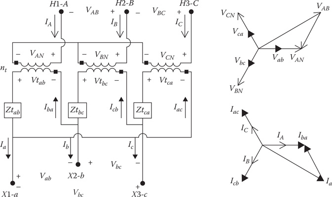
Figure 8.8
Standard ungrounded wye–delta connection step-down.

The basic “ideal” transformer voltage and current equations as a function of the “turn’s ratio” are:

$[\begin{matrix} V_{A N} \\ V_{B N} \\ V_{C N} \end{matrix}] = [\begin{matrix} n_{t} & 0 & 0 \\ 0 & n_{t} & 0 \\ 0 & 0 & n_{t} \end{matrix}] \cdot [\begin{matrix} V_{t}_{_{a b}} \\ V_{t}_{_{b c}} \\ V_{t}_{_{c a}} \end{matrix}]$ (8.47)

where

$n_{t} = \frac{k V_{L N_{rated primary}}}{k V_{L L_{rated secondary}}}$

$[V_{L N_{A B C}}] = [A V] \cdot [V_{t}_{_{a b c}}]$ (8.48)

$[\begin{matrix} I_{A} \\ I_{B} \\ I_{C} \end{matrix}] = \frac{1}{n_{t}} \cdot [\begin{matrix} 1 & 0 & 0 \\ 0 & 1 & 0 \\ 0 & 0 & 1 \end{matrix}] \cdot [\begin{matrix} I_{D_{b a}} \\ I_{D_{c b}} \\ I_{D_{a c}} \end{matrix}]$ (8.49)

$\begin{array}{l} [I_{A B C}] = [A I] \cdot [I_{D_{a b c}}] \\ [I_{D_{a b c}}] = {[A I]}^{- 1} \cdot [I_{A B C}] \end{array}$ (8.50)

Solving Equation 8.48 for the “ideal” delta transformer voltages:

$[V_{t}_{_{a b c}}] = {[A V]}^{- 1} \cdot [V_{L N_{A B C}}]$ (8.51)

The line-to-line voltages at node m as a function of the “ideal” transformer voltages and the delta currents are given by:

$[\begin{matrix} V_{a b} \\ V_{b c} \\ V_{c a} \end{matrix}] = [\begin{matrix} V_{t}_{_{a b}} \\ V_{t}_{_{b c}} \\ V_{t}_{_{c a}} \end{matrix}] - [\begin{matrix} Z_{t}_{_{a b}} & 0 & 0 \\ 0 & Z_{t}_{_{a c}} & 0 \\ 0 & 0 & Z_{t}_{_{c a}} \end{matrix}] \cdot [\begin{matrix} I_{D_{b a}} \\ I_{D_{c b}} \\ I_{D_{a c}} \end{matrix}]$ (8.52)

$[V_{L L_{a b c}}] = [V_{t}_{_{a b c}}] - [Z_{t}_{_{a b c}}] \cdot [I_{D_{_{a b c}}}]$ (8.53)

Substitute Equations 8.50 and 8.51 into Equation 8.53:

$[V_{L L_{a b c}}] = {[A V]}^{- 1} \cdot [V_{L N_{A B C}}] - [Z N_{t}_{_{a b c}}] \cdot [I_{A B C}]$ (8.54)

where

$[Z N_{t}_{_{a b c}}] = [Z_{t}_{_{a b c}}] \cdot {[A I]}^{- 1} = [\begin{matrix} n_{t} \cdot Z_{t}_{_{a b}} & 0 & 0 \\ 0 & n_{t} \cdot Z_{t}_{_{b c}} & 0 \\ 0 & 0 & n_{t} \cdot Z_{t}_{_{c a}} \end{matrix}]$ (8.55)

The line currents on the delta side of the transformer bank as a function of the wye transformer currents are given by:

$[I_{a b c}] = [D i] \cdot [I D_{a b c}]$ (8.56)

where

$[D i] = [\begin{matrix} 1 & 0 & - 1 \\ - 1 & 1 & 0 \\ 0 & - 1 & 1 \end{matrix}]$ (8.57)

Substitute Equation 8.50 into Equation 8.56:

$[I_{a b c}] = [D i] \cdot {[A I]}^{- 1} \cdot [I_{A B C}] = [D Y] \cdot [I_{A B C}]$ (8.58)

where

$[D Y] = [D i] \cdot {[A I]}^{- 1} = [\begin{matrix} n_{t} & 0 & - n_{t} \\ - n_{t} & n_{t} & 0 \\ 0 & - n_{t} & n_{t} \end{matrix}]$ (8.59)

Because the matrix [Di] is singular, it is not possible to use Equation 8.56 to develop an equation relating the wye-side line currents at node n to the delta-side line currents at node m. In order to develop the necessary matrix equation, three independent equations must be written. Two independent KCL equations at the vertices of the delta can be used. Because there is no path for the high-side currents to flow to the ground, they must sum to zero and, therefore, so must the delta currents in the transformer secondary sum to zero. This provides the third independent equation. The resulting three independent equations in matrix form are given by:

$[\begin{matrix} I_{a} \\ I_{b} \\ 0 \end{matrix}] = [\begin{matrix} 1 & 0 & - 1 \\ - 1 & 1 & 0 \\ 1 & 1 & 1 \end{matrix}] \cdot [\begin{matrix} I_{b a} \\ I_{c b} \\ I_{a c} \end{matrix}]$ (8.60)

Solving Equation 8.60 for the delta currents:

$[\begin{matrix} I_{b a} \\ I_{c b} \\ I_{a c} \end{matrix}] = {[\begin{matrix} 1 & 0 & - 1 \\ - 1 & 1 & 0 \\ 1 & 1 & 1 \end{matrix}]}^{- 1} \cdot [\begin{matrix} I_{a} \\ I_{b} \\ 0 \end{matrix}] = \frac{1}{3} \cdot [\begin{matrix} 1 & - 1 & 1 \\ 1 & 2 & 1 \\ - 2 & - 1 & 1 \end{matrix}] \cdot [\begin{matrix} I_{a} \\ I_{b} \\ 0 \end{matrix}]$ (8.61)

$[I_{D_{a b c}}] = [L 0] \cdot [I_{a b 0}]$ (8.62)

Equation 8.62 can be modified to include the phase c current by setting the third column of the [L0] matrix to zero.

$[\begin{matrix} I_{b a} \\ I_{c b} \\ I_{a c} \end{matrix}] = \frac{1}{3} \cdot [\begin{matrix} 1 & - 1 & 0 \\ 1 & 2 & 0 \\ - 2 & - 1 & 0 \end{matrix}] \cdot [\begin{matrix} I_{a} \\ I_{b} \\ I_{c} \end{matrix}]$ (8.63)

$[I_{D_{a b c}}] = [L] \cdot [I_{a b c}]$ (8.64)

Solve Equation 8.50 for [I_ABC], and substitute into Equation 8.64:

$[I_{A B C}] = [A I] \cdot [L] \cdot [I_{a b c}] = [d_{t}] \cdot [I_{a b c}]$ (8.65)

where

$[d_{t}] = [A I] \cdot [L] = \frac{1}{3 \cdot n_{T}} \cdot [\begin{matrix} 1 & - 1 & 0 \\ 1 & 2 & 0 \\ - 2 & - 1 & 0 \end{matrix}]$ (8.66)

Equation 8.66 defines the generalized constant matrix [d_t] for the ungro-unded wye–delta step-down transformer connection. In the process of the derivation, a very convenient Equation 8.63 evolved that can be used anytime the currents in a delta need to be determined knowing the line currents. However, it must be understood that this equation will only work when the delta currents sum to zero, which means an ungrounded neutral on the primary.

The generalized matrices [a_t] and [b_t] can now be developed. Solve Equation 8.54 for [VLN_ABC].

$[V_{L N_{A B C}}] = [A V] \cdot [V_{L L_{a b c}}] + [A V] \cdot [Z N_{t}_{_{a b c}}] \cdot [I_{A B C}]$ (8.67)

Substitute Equation 8.65 into Equation 8.67:

$[V_{L N_{A B C}}] = [A V] \cdot [V_{L L_{a b c}}] + [A V] \cdot [Z N_{t}_{_{a b c}}] \cdot [d_{t}] \cdot [I_{a b c}]$

$[V_{L L_{a b c}}] = [D v] \cdot [V_{L N_{a b c}}]$

where

$[D v] = [\begin{matrix} 1 & - 1 & 0 \\ 0 & 1 & - 1 \\ - 1 & 0 & 1 \end{matrix}]$

$\begin{array}{l} [V_{L N_{A B C}}] = [A V] \cdot [D] \cdot [V_{L N}_{_{a b c}}] + [A V] \cdot [Z N_{t}_{_{a b c}}] \cdot [d_{t}] \cdot [I_{a b c}] \\ [V_{L N_{A B C}}] = [a_{t}] \cdot [V_{L N_{a b c}}] + [b_{t}] \cdot [I_{a b c}] \end{array}$ (8.68)

where

$[a_{t}] = [A V] \cdot [D v] = n_{t} \cdot [\begin{matrix} 1 & - 1 & 0 \\ 0 & 1 & - 1 \\ - 1 & 0 & 1 \end{matrix}]$ (8.69)

$[b_{t}] = [A V] \cdot [Z N_{t}_{_{a b c}}] \cdot [d_{t}] = \frac{n_{t}}{3} \cdot [\begin{matrix} Z_{t}_{_{a b}} & - Z_{t}_{_{a b}} & 0 \\ Z_{t}_{_{b c}} & 2 \cdot Z_{t}_{_{b c}} & 0 \\ - 2 \cdot Z_{t}_{_{c a}} & - Z_{t}_{_{c a}} & 0 \end{matrix}]$ (8.70)

The generalized constant matrices have been developed for computing voltages and currents from the load toward the source (backward sweep). The forward sweep matrices can be developed by referring back to Equation 8.54, which is repeated here for convenience.

$[V_{L L_{a b c}}] = {[A V]}^{- 1} \cdot [V_{L N_{A B C}}] - [Z N_{t}_{_{a b c}}] \cdot [I_{A B C}]$ (8.71)

Equation 8.16 is used to compute the equivalent line-to-neutral voltages as a function of the line-to-line voltages.

$[V_{L N_{a b c}}] = [W] \cdot [V_{L L_{a b c}}]$ (8.72)

Substitute Equation 8.71 into Equation 8.72:

$[V_{L N_{a b c}}] = [W] \cdot {[A V]}^{- 1} \cdot [V_{L N_{_{A B C}}}] - [W] \cdot [Z N_{t}_{_{a b c}}] \cdot [d_{t}] \cdot [I_{a b c}]$

$[V_{L N_{a b c}}] = [A_{t}] \cdot [V_{L N_{A B C}}] - [B_{t}] \cdot [I_{a b c}]$ (8.73)

where

$[A_{t}] = [W] \cdot {[A V]}^{- 1} = \frac{1}{3 \cdot n_{t}} \cdot [\begin{matrix} 2 & 1 & 0 \\ 0 & 2 & 1 \\ 1 & 0 & 2 \end{matrix}]$ (8.74)

$[B_{t}] = [W] \cdot [Z N_{t}_{_{a b c}}] \cdot [d_{t}] = \frac{1}{9} \cdot [\begin{matrix} 2 \cdot Z_{t}_{_{a b}} + Z_{t}_{_{b c}} & 2 \cdot Z_{t}_{_{b c}} - 2 \cdot Z_{t}_{_{a b}} & 0 \\ 2 \cdot Z_{t}_{_{b c}} - 2 \cdot Z_{t}_{_{c a}} & 4 \cdot Z_{t}_{_{b c}} - Z_{t}_{_{c a}} & 0 \\ Z_{t}_{_{a b}} - 4 \cdot Z_{t}_{_{c a}} & - Z_{t}_{_{a b}} - 2 \cdot Z_{t}_{_{c a}} & 0 \end{matrix}]$ (8.75)

The generalized matrices have been developed for the ungrounded wye–delta transformer connection. The derivation has applied basic circuit theory and the basic theories of transformers. The end result of the derivations is to provide an easy method of analyzing the operating characteristics of the transformer connection. Example 8.3 will demonstrate the application of the generalized matrices for this transformer connection.

Example 8.3

Figure 8.9 shows three single-phase transformers in an ungrounded wye–delta step-down connection serving a combination of single-phase and three-phase load in a delta connection. The voltages at the load are balanced three-phase of 240 V line-to-line. The net loading by phase is:

S_ab = 100 kVA at 0.9 lagging power factor

S_bc = S_ca = 50 kVA at 0.8 lagging power factor

The transformers are rated:

Phase A–N: 100 kVA, 7200–240 V, Z = 0.01 + j0.04 per unit

Phases B–N and C–N: 50 kVA, 7200–240 V, Z = 0.015 + j0.035 per unit

images

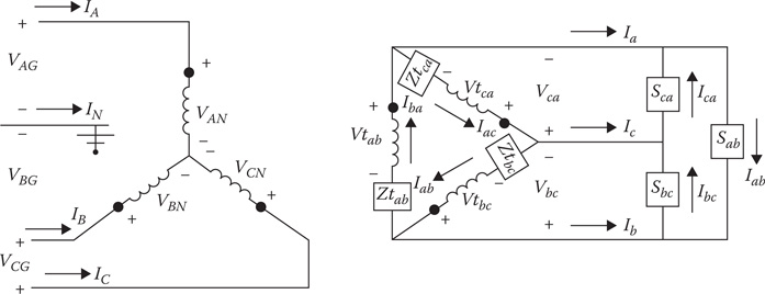
Figure 8.9
Ungrounded wye–delta step-down with unbalanced load.

Determine the following:

The currents in the load
The secondary line currents
The equivalent line-to-neutral secondary voltages
The primary line-to-neutral and line-to-line voltages
The primary line currents

Before the analysis can start, the transformer impedances must be converted to actual values in ohms and located inside the delta-connected secondary windings.“Lighting” transformer:

$Z_{base} = \frac{{0.24}^{2} \cdot 1000}{100} = 0.576$

$Z_{t}_{_{a b}} = (0.01 + j 0.4) \cdot 0.576 = 0.0058 + j .023 Ω$

“Power” transformers:

$Z_{base} = \frac{{0.24}^{2} \cdot 1000}{50} = 1.152$

$Z_{t}_{_{b c}} = Z_{t}_{_{c a}} = (0.015 + j 0.35) \cdot 1.152 = 0.0173 + j 0.0403 Ω$

The transformer impedance matrix can now be defined:

$[Z_{t}_{_{a b c}}] = [\begin{matrix} 0.0058 + j .023 & 0 & 0 \\ 0 & 0.0173 + j .0403 & 0 \\ 0 & 0 & 0.0173 + j .0403 \end{matrix}] Ω$

The turn’s ratio of the transformers is: $n_{t} = \frac{7200}{240} = 30$

Define all of the matrices:

$[W] = \frac{1}{3} \cdot [\begin{matrix} 2 & 1 & 0 \\ 0 & 2 & 1 \\ 1 & 0 & 2 \end{matrix}] [D v] = [\begin{matrix} 1 & - 1 & 0 \\ 0 & 1 & - 1 \\ - 1 & 0 & 1 \end{matrix}] [D i] = [\begin{matrix} 1 & 0 & - 1 \\ - 1 & 1 & 0 \\ 0 & - 1 & 1 \end{matrix}]$

$[a_{t}] = n_{t} \cdot [\begin{matrix} 1 & - 1 & 0 \\ 0 & 1 & - 1 \\ - 1 & 0 & 1 \end{matrix}] = [\begin{matrix} 30 & - 30 & 0 \\ 0 & 30 & - 30 \\ - 30 & 0 & 30 \end{matrix}]$

$[b_{t}] = \frac{n_{t}}{3} \cdot [\begin{matrix} Z_{t}_{_{a b}} & - Z_{t}_{_{a b}} & 0 \\ Z_{t}_{_{b c}} & 2 \cdot Z_{t}_{_{b c}} & 0 \\ - 2 \cdot Z_{t}_{_{c a}} & - Z_{t}_{_{c a}} & 0 \end{matrix}] = [\begin{matrix} 0.0576 + j .2304 & - 0.576 - j .2304 & 0 \\ 0.1728 + j .4032 & 0.3456 + j .8064 & 0 \\ - 0.3456 - j .8064 & - 0.1728 - j .4032 \end{matrix}]$

$[c_{t}] = [\begin{matrix} 0 & 0 & 0 \\ 0 & 0 & 0 \\ 0 & 0 & 0 \end{matrix}]$

$[d_{t}] = \frac{1}{3 \cdot n_{T}} \cdot [\begin{matrix} 1 & - 1 & 0 \\ 1 & 2 & 0 \\ - 2 & - 1 & 0 \end{matrix}] = [\begin{matrix} 0.0111 & - 0.0111 & 0 \\ 0.0111 & 0.0222 & 0 \\ - 0.0222 & - 0.0111 \end{matrix}]$

$[A_{t}] = \frac{1}{3 \cdot n_{t}} \cdot [\begin{matrix} 2 & 1 & 0 \\ 0 & 2 & 1 \\ 1 & 0 & 2 \end{matrix}] = [\begin{matrix} 0.0222 & 0.0111 & 0 \\ 0 & 0.0222 & 0.0111 \\ 0.0111 & 0 & 0.0222 \end{matrix}]$

$[B_{t}] = \frac{1}{9} \cdot [\begin{matrix} 2 \cdot Z_{t}_{_{a b}} + Z_{t}_{_{b c}} & 2 \cdot Z_{t}_{_{b c}} - 2 \cdot Z_{t}_{_{a b}} & 0 \\ 2 \cdot Z_{t}_{_{b c}} - 2 \cdot Z_{t}_{_{c a}} & 4 \cdot Z_{t}_{_{b c}} - Z_{t}_{_{c a}} & 0 \\ Z_{t}_{_{a b}} - 4 \cdot Z_{t}_{_{c a}} & - Z_{t}_{_{a b}} - 2 \cdot Z_{t}_{_{c a}} & 0 \end{matrix}]$

$[B_{t}] = [\begin{matrix} 0.0032 + j .0096 & 0.0026 + j .0038 & 0 \\ 0 & 0.0058 + j .0134 & 0 \\ - 0.007 - j .0154 & - 0.0045 - j .0115 & 0 \end{matrix}]$

Define the line-to-line load voltages:

$[V_{L L}_{_{a b c}}] = [\begin{matrix} 240 \underset{__}{/ 0} \\ 240 \underset{_____}{/ - 120} \\ 240 \underset{_____}{/ 120} \end{matrix}] V$

Define the loads:

$[S D_{a b c}] = [\begin{matrix} 100 \underset{_____}{/ acos (0.9)} \\ 50 \underset{_____}{/ acos (0.8)} \\ 50 \underset{_____}{/ acos (0.8)} \end{matrix}] = [\begin{matrix} 90 + j 43.589 \\ 40 + j 30 \\ 40 + j 30 \end{matrix}] kVA$

Calculate the delta load currents:

$I_{D}_{_{i}} = {(\frac{S D_{i} \cdot 1000}{V_{L L}_{{_{a b c}}_{_{i}}}})}^{*} A$

$[I_{D}_{_{a b c}}] = [\begin{matrix} I_{a b} \\ I_{b c} \\ I_{c a} \end{matrix}] = [\begin{matrix} 416.7 \underset{_____}{/ - 25.84} \\ 208.3 \underset{_____}{/ - 156.87} \\ 208.3 \underset{_____}{/ 83.13} \end{matrix}] A$

Compute the secondary line currents:

$[I_{a b c}] = [D i] \cdot [I_{D}_{_{a b c}}] = [\begin{matrix} 522.9 \underset{_____}{/ - 47.97} \\ 575.3 \underset{_____}{/ - 119.06} \\ 360.8 \underset{_____}{/ 53.13} \end{matrix}] A$

Compute the equivalent secondary line-to-neutral voltages:

$[V_{L N}_{_{a b c}}] = [W] \cdot [V_{L L}_{_{a b c}}] = [\begin{matrix} 138.56 \underset{_____}{/ - 30} \\ 138.56 \underset{_____}{/ - 150} \\ 138.56 \underset{_____}{/ 90} \end{matrix}] A$

Use the generalized constant matrices to compute the primary line-to-neutral voltages and line-to-line voltages:

$[V_{L N}_{_{A B C}}] = [a_{t}] \cdot [V_{L N}_{_{a b c}}] + [b_{t}] \cdot [I_{a b c}] = [\begin{matrix} 7367.6 \underset{_____}{/ 1.4} \\ 7532.3 \underset{_____}{/ - 119.1} \\ 7406.2 \underset{_____}{/ 121.7} \end{matrix}] V$

$[V_{L L}_{_{A B C}}] = [D v] \cdot [V_{L N}_{_{A B C}}] = [\begin{matrix} 12, 9356 \underset{_____}{/ 31.54} \\ 12, 8845 \underset{_____}{/ - 88.95} \\ 12, 8147 \underset{_____}{/ 151.50} \end{matrix}] kV$

The high primary line currents are:

$[I_{A B C}] = [d_{t}] \cdot [I_{a b c}] = [\begin{matrix} 11.54 \underset{_____}{/ - 28.04} \\ 8.95 \underset{_____}{/ - 166.43} \\ 7.68 \underset{_____}{/ 101.16} \end{matrix}] A$

It is interesting to compute the operating kVA of the three transformers. Taking the product of the transformer voltage times the conjugate of the current gives the operating kVA of each transformer.

$S T_{i} = {\frac{V_{L N}_{{_{A B C}}_{_{i}}} \cdot (I_{A B C_{i}})}{1000}}^{*} = [\begin{matrix} 85.02 \underset{_____}{/ 29.46} \\ 67.42 \underset{_____}{/ 47.37} \\ 56.80 \underset{_____}{/ 20.58} \end{matrix}] kVA$

The operating power factors of the three transformers are:

$[P F] = [\begin{matrix} \cos (29.46) \\ \cos (47.37) \\ \cos (20.58) \end{matrix}] = [\begin{matrix} 87.1 \\ 67.7 \\ 93.6 \end{matrix}] %$

Note that the operating kVAs do not match very closely with the rated kVAs of the three transformers. In particular, the transformer on phase A did not serve the total load of 100 kVA that is directly connected to its terminals. That transformer is operating below the rated kVA, whereas the other two transformers are overloaded. In fact, the transformer connected to phase B is operating 35% above the rated kVA. Because of this overload, the ratings of the three transformers should be changed so that the phase B and phase C transformers are rated 75 kVA. Finally, the operating power factors of the three transformers bear little resemblance to the load power factors.

Example 8.3 demonstrates how the generalized constant matrices can be used to determine the operating characteristics of the transformers. In addition, the example shows that the obvious selection of transformer ratings will lead to an overload condition on the two power transformers. The advantage in this is that if the generalized constant matrices have been applied in a computer program, it is simple to change the transformer kVA ratings, and we can be assured that none of the transformers will be operating in an overload condition.

Example 8.3 has demonstrated the “backward” sweep to compute the primary voltages and currents. As before, when the source (primary) voltages are given along with the load PQ, the ladder iterative technique must be used to analyze the transformer connection.

Example 8.4

The Mathcad program that has been used in previous examples is modified to demonstrate the ladder iterative technique for computing the load voltages given the source voltages and load power and reactive powers (PQ load). In Example 8.4, the computed source voltages from Example 8.3 are specified along with the same loads. From Example 8.3, the source voltages are:

$[V_{L L}_{_{A B C}}] = [\begin{matrix} 12, 935.6 \underset{_____}{/ 31.5} \\ 12, 884.5 \underset{_____}{/ - 88.9} \\ 12, 814.7 \underset{_____}{/ 151.5} \end{matrix}]$

The initial conditions are:

$[Start] = [\begin{matrix} 0 \\ 0 \\ 0 \end{matrix}] T o l = 0.000001 V M = 240$

The modified Mathcad program is shown in Figure 8.10.

With balanced source voltages specified, after six iterations the load voltages are computed to be exactly as they were specified in Example 8.3:

$[V_{L L}_{_{a b c}}] = [\begin{matrix} 240 \underset{__}{/ 0} \\ 240 \underset{_____}{/ - 120} \\ 240.0 \underset{_____}{/ 120} \end{matrix}] V$

images

Figure 8.10
Mathcad program.

Example 8.4 has demonstrated how the simple Mathcad program can be modified to analyze the ungrounded wye–delta step-down transformer bank connection.

8.6 The Ungrounded Wye–Delta Step-Up Connection

The connection diagram for the step-up connection is shown in Figure 8.11.

The only difference in the matrices between the step-up and step-down connections is the definitions of the turn’s ratio n_t, [AV] and [AV]. For the step-up connection:

$n_{t} = \frac{k V_{L N}_{_{rated primary}}}{k V_{L L}_{_{rated secondary}}}$ (8.76)

$\begin{array}{l} [\begin{matrix} V_{A N} \\ V_{B N} \\ V_{C N} \end{matrix}] = n_{t} \cdot [\begin{matrix} 0 & 0 & - 1 \\ - 1 & 0 & 0 \\ 0 & - 1 & 0 \end{matrix}] \cdot [\begin{matrix} V_{t}_{_{a b}} \\ V_{t}_{_{b c}} \\ V_{t}_{_{c a}} \end{matrix}] \\ [V_{L N}_{_{A B C}}] = [A V] \cdot [V_{t}_{_{a b c}}] \end{array}$ (8.77)

where

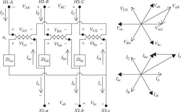
$[A V] = n_{t} \cdot [\begin{matrix} 0 & 0 & - 1 \\ - 1 & 0 & 0 \\ 0 & - 1 & 0 \end{matrix}]$

images

Figure 8.11
Ungrounded wye–delta step-up connection.

$\begin{array}{l} [\begin{matrix} I_{A} \\ I_{B} \\ I_{C} \end{matrix}] = \frac{1}{n_{t}} \cdot [\begin{matrix} 0 & 0 & - 1 \\ - 1 & 0 & 0 \\ 0 & - 1 & 0 \end{matrix}] \cdot [\begin{matrix} I_{D}_{_{b a}} \\ I_{D}_{_{c b}} \\ I_{D}_{_{a c}} \end{matrix}] \\ [I_{A B C}] = [A I] \cdot [I_{D}_{_{a b c}}] \end{array}$ (8.78)

where

$[A I] = \frac{1}{n_{t}} \cdot [\begin{matrix} 0 & 0 & - 1 \\ - 1 & 0 & 0 \\ 0 & - 1 & 0 \end{matrix}]$

Example 8.5

The equations for the forward and backward sweep matrices, as defined in Section 8.3, can be applied using the definitions in Equations 8.76, 8.77, and 8.77. The system in Example 8.3 is modified so that transformer connection is step up. The transformers have the same ratings, but now the rated voltages for the primary and secondary are:

$\begin{array}{l} Primary: V_{L L}_{_{pri}} = 240 V_{L N}_{_{pri}} = 138.6 V \\ Secondary: V_{L L}_{_{\sec}} = 12, 470 V \\ n_{t} = \frac{V_{L N}_{_{pri}}}{V_{L L}_{_{\sec}}} = \frac{138.6}{12, 470} = 0.0111 \end{array}$

The transformer impedances must be computed in Ohms relative to the delta secondary and then used to compute the new forward and backward sweep matrices. When this is done, the new matrices are:

$\begin{array}{l} [d_{t}] = {[A I]}^{- 1} \cdot [L] = [\begin{matrix} 60 & 30 & 0 \\ - 30 & 30 & 0 \\ - 30 & - 60 & 0 \end{matrix}] \\ [A_{t}] = [W] \cdot {[A V]}^{- 1} = [\begin{matrix} 0 & - 60 & - 30 \\ - 30 & 0 & - 60 \\ - 60 & - 30 & 0 \end{matrix}] \\ [B_{t}] = [W] \cdot [Z N_{t}_{_{a b c}}] \cdot [d_{t}] = [\begin{matrix} 8.64 + j 25.92 & 6.91 + j 10.37 & 0 \\ 0 & 15.55 + j 36.28 & 0 \\ - 19.01 - j 41.47 & - 12.09 - j 31.10 & 0 \end{matrix}] \end{array}$

Using these matrices aAU: Please check if there any missing text in this sentence.nd the same loads, specify the primary line-to-line voltages to be:

$[V_{L L}_{_{A B C}}] = [\begin{matrix} 240 \underset{_____}{/ 30} \\ 240 \underset{_____}{/ - 90} \\ 240 \underset{_____}{/ 150} \end{matrix}]$

Using the Mathcad program in Figure 8.9, the Ladder iterative technique computes the load voltages as:

$[V_{L L}_{_{a b c}}] = [\begin{matrix} 12, 055 \underset{_____}{/ 58.2} \\ 11, 982 \underset{_____}{/ - 61.3} \\ 12, 106 \underset{_____}{/ 178.7} \end{matrix}]$

8.7 The Grounded Wye–Delta Step-Down Connection

The Connection diagram for the standard 30° grounded wye (high)–delta (low) transformer connection grounded through an impedance of Z_g is shown in Figure 8.12. Note that the primary is grounded through an impedance of Z_g.

images

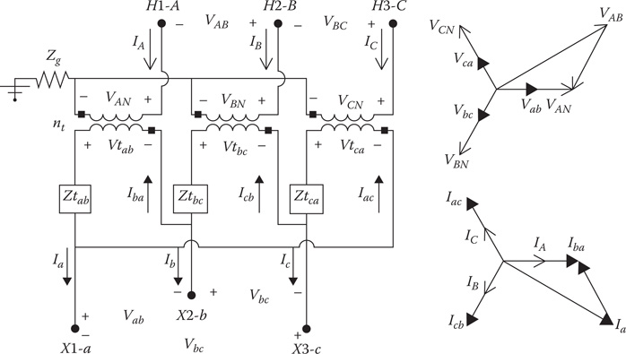
Figure 8.12
The grounded wye–delta connection.

Basic transformer equations:

The turn’s ratio is given by:

$n_{t} = \frac{k V L N_{_{rated primary}}}{k V L L_{_{rated secondary}}}$ (8.79)

The basic “ideal” transformer voltage and current equations as a function of the turn’s ratio are:

$\begin{array}{l} [\begin{matrix} V_{A N} \\ V_{B N} \\ V_{C N} \end{matrix}] = n_{t} \cdot [\begin{matrix} 1 & 0 & 0 \\ 0 & 1 & 0 \\ 0 & 0 & 1 \end{matrix}] \cdot [\begin{matrix} V_{t}_{_{a b}} \\ V_{t}_{_{b c}} \\ V_{t}_{_{c a}} \end{matrix}] \\ [V_{L N}_{_{A B C}}] = [A V] \cdot [V_{t}_{_{a b c}}] \end{array}$ (8.80)

where

$[A V] = n_{t} \cdot [\begin{matrix} 1 & 0 & 0 \\ 0 & 1 & 0 \\ 0 & 0 & 1 \end{matrix}]$

$\begin{array}{l} [\begin{matrix} I_{A} \\ I_{B} \\ I_{C} \end{matrix}] = \frac{1}{n_{t}} \cdot [\begin{matrix} 1 & 0 & 0 \\ 0 & 1 & 0 \\ 0 & 0 & 1 \end{matrix}] \cdot [\begin{matrix} I_{D}_{_{b a}} \\ I_{D}_{_{c b}} \\ I_{D}_{_{a c}} \end{matrix}] \\ [I_{A B C}] = [A I] \cdot [I_{D}_{_{a b c}}] \\ [I_{D}_{_{a b c}}] = {[A I]}^{- 1} \cdot [I_{A B C}] \end{array}$ (8.81)

where

$[A I] = \frac{1}{n_{t}} \cdot [\begin{matrix} 1 & 0 & 0 \\ 0 & 1 & 0 \\ 0 & 0 & 1 \end{matrix}]$

Solving Equation 8.80 for the “ideal” transformer voltages:

$[V_{t}_{_{a b c}}] = {[A V]}^{- 1} \cdot [V_{L N}_{_{A B C}}]$ (8.82)

The line-to-neutral transformer primary voltages as a function of the system line-to-ground voltages are given by:

$\begin{array}{l} V_{A N} = V_{A G} - Z_{g} \cdot (I_{A} + I_{B} + I_{C}) \\ V_{B N} = V_{B G} - Z_{g} \cdot (I_{A} + I_{B} + I_{C}) \\ V_{C N} = V_{C G} - Z_{g} \cdot (I_{A} + I_{B} + I_{C}) \\ [\begin{matrix} V_{A N} \\ V_{B N} \\ V_{C N} \end{matrix}] = [\begin{matrix} V_{A G} \\ V_{B G} \\ V_{C G} \end{matrix}] - [\begin{matrix} Z_{g} & Z_{g} & Z_{g} \\ Z_{g} & Z_{g} & Z_{g} \\ Z_{g} & Z_{g} & Z_{g} \end{matrix}] \cdot [\begin{matrix} I_{A} \\ I_{B} \\ I_{C} \end{matrix}] \\ [V_{L N}_{_{A B C}}] = [V_{L G}_{_{A B C}}] - [Z G] \cdot [I_{A B C}] \end{array}$ (8.83)

where

$[Z G] = [\begin{matrix} Z_{g} & Z_{g} & Z_{g} \\ Z_{g} & Z_{g} & Z_{g} \\ Z_{g} & Z_{g} & Z_{g} \end{matrix}]$

The line-to-line voltages on the delta side are given by:

$\begin{array}{l} [\begin{matrix} V_{a b} \\ V_{b c} \\ V_{c a} \end{matrix}] = [\begin{matrix} V_{t}_{_{a}} \\ V_{t}_{_{b}} \\ V_{t}_{_{c}} \end{matrix}] - [\begin{matrix} Z_{t}_{_{a b}} & 0 & 0 \\ 0 & Z_{t}_{_{b c}} & 0 \\ 0 & 0 & Z_{t}_{_{c a}} \end{matrix}] \cdot [\begin{matrix} I_{D}_{_{b a}} \\ I_{D}_{_{c b}} \\ I_{D}_{_{a c}} \end{matrix}] \\ [V_{L L}_{_{a b c}}] = [V_{t}_{_{a b c}}] - [Z_{t}_{_{a b c}}] \cdot [I_{D}_{_{a b c}}] \end{array}$ (8.84)

Substitute Equation 8.82 into 8.84:

$[V_{L L}_{_{a b c}}] = {[A V]}^{- 1} \cdot [V_{L N}_{_{A B C}}] - [Z_{t}_{_{a b c}}] \cdot [I_{D}_{_{a b c}}]$ (8.85)

Substitute Equation 8.81 into 8.85:

$[V_{L L}_{_{a b c}}] = {[A V]}^{- 1} \cdot [V_{L N}_{_{A B C}}] - [Z_{t}_{_{a b c}}] \cdot [I_{D}_{_{a b c}}]$ (8.86)

Substitute Equation 8.83 into Equation 8.86:

$\begin{matrix} {[VLL}_{a b c} {]=[AV]}^{- 1} . ([V L G_{A B C}] - [Z G] . [I_{A B C}]) - ([Z t_{a b c}] . {[AI]}^{- 1}) . [I_{A B C}] \\ {[VLL}_{a b c} {]=[AV]}^{- 1} . [V L G_{A B C}] - ({[A V]}^{- 1} . [Z G]) + [Z t_{a b c}] . {[A I]}^{- 1}) . [I_{A B C}] \end{matrix}$ (8.87)

Equation 8.81 gives the delta secondary currents as a function of the primary wye-side line currents. The secondary line currents are related to the secondary delta currents by:

$[\begin{matrix} I_{a} \\ I_{b} \\ I_{c} \end{matrix}] = [\begin{matrix} 1 & 0 & - 1 \\ - 1 & 1 & 0 \\ 0 & - 1 & 1 \end{matrix}] \cdot [\begin{matrix} I_{D}_{_{b a}} \\ I_{D}_{_{c b}} \\ I_{D}_{_{a c}} \end{matrix}] [I_{a b c}] = [D i] \cdot [I_{D}_{_{a b c}}]$ (8.88)

The real problem of transforming currents from one side to the other occurs for the case when the line currents on the delta secondary side [I_abc] are known and the transformer secondary currents [ID_abc] and primary line currents on the wye side [I_ABC] are needed. The only way a relationship can be developed is to recognize that the sum of the line-to-line voltages on the delta secondary of the transformer bank must add up to zero. Three independent equations can be written as follows:

$\begin{array}{l} I_{a} = I_{b a} - I_{a c} \\ I_{b} = I_{c b} - I_{b a} \end{array}$ (8.89)

KVL around the delta secondary windings gives:

$V_{t_{a b}} - Z_{t}_{_{a b}} \cdot I_{b a} + V_{t}_{_{b c}} - Z_{t}_{_{b c}} \cdot I_{c b} + V_{t}_{_{c a}} - Z_{t}_{_{c a}} \cdot I_{a c} = 0$ (8.90)

Replacing the “ideal” secondary delta voltages with the primary line-to-neutral voltages:

$\frac{V_{A N}}{n_{t}} + \frac{V_{B N}}{n_{t}} + \frac{V_{C N}}{n_{t}} = Z_{t}_{_{a b}} \cdot I_{b a} + Z_{t}_{_{b c}} \cdot I_{c b} + Z_{t}_{_{c a}} \cdot I_{a c}$ (8.91)

Multiply both sides of the Equation 8.91 by the turn’s ratio n_t:

$V_{A N} + V_{B N} + V_{C N} = n_{t} \cdot Z_{t}_{_{a b}} \cdot I_{b a} + n_{t} \cdot Z_{t}_{_{b c}} \cdot I_{c b} + n_{t} \cdot Z_{t}_{_{c a}} \cdot I_{a c}$ (8.92)

Determine the left side of Equation 8.92 as a function of the line-to-ground voltages using Equation 8.83:

$\begin{array}{l} V_{A N} + V_{B N} + V_{C N} = V_{A G} + V_{B G} + V_{C G} - 3 \cdot Z_{g} \cdot (I_{A} + I_{B} + I_{C}) \\ V_{A N} + V_{B N} + V_{C N} = V_{A G} + V_{B G} + V_{C G} - 3 \cdot \frac{1}{n_{t}} \cdot Z_{g} \cdot (I_{b a} + I_{c b} + I_{a c}) \end{array}$ (8.93)

Substitute Equation 8.93 into Equation 8.92:

$\begin{array}{l} V_{A G} + V_{B G} + V_{C G} - \frac{3}{n_{t}} \cdot Z_{g} \cdot (I_{b a} + I_{c b} + I_{a c}) = n_{t} \cdot Z_{t}_{_{a b}} \cdot I_{b a} + n_{t} \cdot Z_{t}_{_{b c}} \cdot I_{c b} + n_{t} \cdot Z_{t}_{_{c a}} \cdot I_{a c} \\ V_{sum} = (n_{t} \cdot Z_{t}_{_{a b}} + \frac{3}{n_{t}} \cdot Z_{g}) \cdot I_{b a} + (n_{t} \cdot Z_{t}_{_{b c}} + \frac{3}{n_{t}} \cdot Z_{g}) \cdot I_{c b} + (n_{t} \cdot Z_{t}_{_{c a}} + \frac{3}{n_{t}} \cdot Z_{g}) \cdot I_{a c} \end{array}$ (8.94)

where

$V_{sum} = V_{A G} + V_{B G} + V_{C G}$

Equations 8.88, 8.89, and 8.94 can be put into matrix form:

$[\begin{matrix} I_{a} \\ I_{b} \\ V_{sum} \end{matrix}] = [\begin{matrix} 1 & 0 & - 1 \\ - 1 & 1 & 0 \\ n_{t} \cdot Z_{t}_{_{a b}} + \frac{3}{n_{t}} \cdot Z_{g} & n_{t} \cdot Z_{t}_{_{b c}} + \frac{3}{n_{t}} \cdot Z_{g} & n_{t} \cdot Z_{t}_{_{c a}} + \frac{3}{n_{t}} \cdot Z_{g} \end{matrix}] \cdot [\begin{matrix} I_{b a} \\ I_{c b} \\ I_{a c} \end{matrix}]$ (8.95)

Equation 8.95 in general form is:

$[X] = [F] \cdot [I_{D}_{_{a b c}}]$ (8.96)

Solve for [ID_abc]:

$[I_{D}_{_{a b c}}] = {[F]}^{- 1} \cdot [X] = [G] \cdot [X]$ (8.97)

Equation 8.97 in full form is:

$\begin{array}{l} [I_{D}_{_{a b c}}] = [\begin{matrix} G_{11} & G_{12} & G_{13} \\ G_{21} & G_{22} & G_{23} \\ G_{31} & G_{32} & G_{33} \end{matrix}] \cdot [\begin{matrix} I_{a} \\ I_{b} \\ V_{A G} + V_{B G} + V_{C G} \end{matrix}] \\ [I_{D}_{_{a b c}}] = [\begin{matrix} G_{13} & G_{13} & G_{13} \\ G_{23} & G_{23} & G_{23} \\ G_{33} & G_{33} & G_{33} \end{matrix}] \cdot [\begin{matrix} V_{A G} \\ V_{B G} \\ V_{C G} \end{matrix}] + [\begin{matrix} G_{11} & G_{12} & 0 \\ G_{21} & G_{22} & 0 \\ G_{31} & G_{32} & 0 \end{matrix}] \cdot [\begin{matrix} I_{a} \\ I_{b} \\ I_{c} \end{matrix}] \end{array}$ (8.98)

Equation 8.98 in shortened form is:

$[I_{D}_{_{a b c}}] = [G_{1}] \cdot [V_{L G}_{_{A B C}}] + [G_{2}] \cdot [I_{a b c}]$ (8.99)

Substitute Equation 8.81 into Equation 8.98:

$\begin{array}{l} [I_{A B C}] = [A I] \cdot [I_{D}_{_{a b c}}] = [A I] \cdot ([G_{1}] \cdot [V_{L G}_{_{A B C}}] + [G_{2}] \cdot [I_{a b c}]) \\ [I_{A B C}] = [x_{t}] \cdot [V_{L G}_{_{A B C}}] + [d_{t}] \cdot [I_{a b c}] \end{array}$ (8.100)

where

$\begin{array}{l} [x_{t}] = [A I] \cdot [G_{1}] \\ [d_{t}] = [A I] \cdot [G_{2}] \end{array}$

Equation 8.100 is used in the “backward” sweep to compute the primary currents based upon the secondary currents and primary LG voltages.

The “forward” sweep equation is determined by substituting Equation 8.100 into Equation 8.87.

$\begin{array}{l} [V L L_{a b c}] = {[A V]}^{- 1} \cdot [V L G_{A B C}] - ([A V]^{- 1} \cdot [Z G] + [Z t_{a b c}] \cdot {[A I]}^{- 1}) \cdot [I_{A B C}] \\ [V L L_{a b c}] = [A V]^{- 1} \cdot [V L G_{A B C}] - ([Z t_{a b c}] \cdot [A I]^{- 1} + [A V]^{- 1} \cdot [Z G]) \cdot ([X_{t}] \cdot [V L G_{A B C}] + [d_{t}] \cdot [I_{a b c}]) \\ D e f i n e : [X_{1}]=[Z t_{a b c}] \cdot [A I]^{- 1} + [A V]^{- 1} \cdot [Z G] \\ [V L L_{a b c}] = [A V] - [X_{1}] \cdot [X_{t}] \cdot ([V L G_{A B C}] - [X_{1}] \cdot [d_{t}] \cdot [I_{a b c}]) \\ [V L N_{a b c}] = [W] \cdot [V L L_{a b c}] \\ [V L N_{a b c}] = [W] \cdot (([A V]^{- 1} - [X_{1}] \cdot [X_{t}]) \cdot [V L G_{A B C}] - [X_{1}] \cdot [d_{t}] \cdot [I_{a b c}]) \\ [V L N_{a b c}] = [W] \cdot ([A V]^{- 1} - [X_{1}] \cdot [X_{t}]) \cdot [V L G_{A B C}] - [W] [X_{1}] \cdot [d_{t}] \cdot [I_{a b c}] \end{array}$ (8.101)

The final form of Equation 8.101 gives the equation for the forward sweep.

$[V_{L N}_{_{a b c}}] = [A_{t}] \cdot [V_{L G}_{_{A B C}}] - [B_{t}] \cdot [I_{a b c}]$ (8.102)

where

$\begin{array}{l} [A_{t}] = [W] \cdot ({[A V]}^{- 1} - [X_{1}] \cdot [x_{t}]) \\ [B_{t}] = [W] \cdot [X_{1}] \cdot [d_{t}] \end{array}$

Example 8.6

The system in Examples 8.3 and 8.4 is changed so that the same transformers are connected in a grounded wye–delta step-down connection to serve the same load. The neutral ground resistance is 5 Ω. The computed matrices are:

$[x_{t}] = [\begin{matrix} 0.0053 - j 0.0061 & 0.0053 - j 0.0061 & 0.0053 - j 0.0061 \\ 0.0053 - j 0.0061 & 0.0053 - j 0.0061 & 0.0053 - j 0.0061 \\ 0.0053 - j 0.0061 & 0.0053 - j 0.0061 & 0.0053 - j 0.0061 \end{matrix}]$

$[d_{t}] = [\begin{matrix} 0.0128 + j 0.0002 & - 0.0128 - j 0.0002 & 0 \\ 0.0128 + j 0.0002 & 0.0206 - j 0.0002 & 0 \\ - 0.0206 + j 0.0002 & - 0.0128 - j 0.0002 & 0 \end{matrix}]$

$[A_{t}] = [\begin{matrix} 0.0128 + j 0.0002 & 0.0017 + j 0.0002 & - 0.0094 + j 0.0002 \\ - 0.0128 - j 0.0002 & 0.0094 - j 0.0002 & - 0.0017 - j 0.0002 \\ 0 & - 0.0111 & 0.0111 \end{matrix}]$

$[B_{t}] = [\begin{matrix} 0.0043 + j 0.0112 & 0.0014 + j 0.0022 & 0 \\ 0.0014 + j 0.0022 & 0.0043 + j 0.0112 & 0 \\ - 0.0058 - j 0.0134 & - 0.0058 - j 0.0134 & 0 \end{matrix}]$

The only change in the program from Example 8.4 is for the equation computing the primary line currents.

$[I_{A B C}] = [x_{t}] \cdot [V_{L G}_{_{A B C}}] + [d_{t}] \cdot [I_{a b c}]$

The source voltages are balanced of 12,470 V. After five iterations, the resulting load line-to-line load voltages are:

$[V_{L L}_{_{a b c}}] = [\begin{matrix} 232.6 \underset{_____}{/ - 1.7} \\ 231.0 \underset{_____}{/ - 121.4} \\ 233.0 \underset{_____}{/ 118.8} \end{matrix}]$

The voltage unbalance is computed to be:

$V_{unbalance} = 0.53 %$

The currents are:

$\begin{array}{l} [I_{a b c}] = [\begin{matrix} 540.8 \underset{_____}{/ - 49.5} \\ 594.1 \underset{_____}{/ 168.5} \\ 373.0 \underset{_____}{/ 51.7} \end{matrix}] \\ [I_{A B C}] = [\begin{matrix} 13.7 \underset{_____}{/ - 28.6} \\ 7.8 \underset{_____}{/ - 160.4} \\ 7.1 \underset{_____}{/ 87.3} \end{matrix}] \\ I_{g} = - (I_{A} + I_{B} + I_{C}) = 5.4 \underset{_____}{/ 157.8} \end{array}$

As can be seen, the major difference between this and the ungrounded connection is in the line currents and the ground current on the primary side. Experience has shown that the value of the neutral grounding resistance should not exceed the transformer impedance relative to the primary side. If the ground resistance is too big, the program will not converge.The question can be whether the neutral for the wye–delta connection can be grounded or not. In Chapter 10, the short-circuit calculations for the grounded wye–delta transformer bank will be developed. In this development, it will be shown that during a grounded fault upstream from the transformer bank, there will be a back feed current from the grounded wye–delta bank back to the grounded fault. This typically results in blowing the transformer fuses for the upstream ground fault. With that in mind, the grounded wye–delta transformer connection should not be used.

8.8 Open Wye–Open Delta

A common load to be served on a distribution feeder is a combination of a single-phase lighting load and a three-phase power load. Mostly, the three-phase power load will be an induction motor. This combination load can be served by a grounded or ungrounded wye–delta connection as previously described or by an “open wye–open delta” connection. When the three-phase load is small compared to the single-phase load, the open wye–open delta connection is commonly used. The open wye–open delta connection requires only two transformers, but the connection will provide three-phase line-to-line voltages to the combination load. Figure 8.13 shows the open wye–open delta connection and the primary and secondary positive sequence voltage phasors.

images

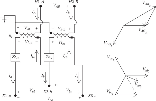
Figure 8.13
Open wye–open delta connection.

With reference to Figure 8.11, the basic “ideal” transformer voltages as a function of the “turn’s ratio” are:

$\begin{array}{l} [\begin{matrix} V_{A G} \\ V_{B G} \\ V_{C G} \end{matrix}] = n_{t} \cdot [\begin{matrix} 1 & 0 & 0 \\ 0 & 1 & 0 \\ 0 & 0 & 0 \end{matrix}] \cdot [\begin{matrix} V_{t}_{_{a b}} \\ V_{t}_{_{b c}} \\ V_{t}_{_{c a}} \end{matrix}] \\ [V_{L G}_{_{A B C}}] = [A V] \cdot [V_{t}_{_{a b c}}] \end{array}$ (8.103)

The currents as a function of the turn’s ratio are given by:

$\begin{array}{l} I_{A} = \frac{1}{n_{t}} \cdot I_{b a} = \frac{1}{n_{t}} \cdot I_{a} \\ I_{B} = \frac{1}{n_{t}} \cdot I_{c b} = - \frac{1}{n_{t}} \cdot I_{c} \\ I_{b} = - (I_{a} + I_{c}) \end{array}$ (8.104)

Equation 8.104 can be expressed in matrix form by:

$\begin{array}{l} [\begin{matrix} I_{A} \\ I_{B} \\ I_{C} \end{matrix}] = \frac{1}{n_{t}} \cdot [\begin{matrix} 1 & 0 & 0 \\ 0 & 0 & - 1 \\ 0 & 0 & 0 \end{matrix}] \cdot [\begin{matrix} I_{a} \\ I_{b} \\ I_{c} \end{matrix}] \\ [I_{A B C}] = [d_{t}] \cdot [I_{a b c}] \end{array}$ (8.105)

where

$[d_{t}] = \frac{1}{n_{t}} \cdot [\begin{matrix} 1 & 0 & 0 \\ 0 & 0 & - 1 \\ 0 & 0 & 0 \end{matrix}]$

The secondary line currents as a function of the primary line currents are:

$\begin{array}{l} [\begin{matrix} I_{a} \\ I_{b} \\ I_{c} \end{matrix}] = n_{t} \cdot [\begin{matrix} 1 & 0 & 0 \\ - 1 & 1 & 0 \\ 0 & - 1 & 0 \end{matrix}] \cdot [\begin{matrix} I_{A} \\ I_{B} \\ I_{C} \end{matrix}] \\ [I_{a b c}] = [A i] \cdot [I_{A B C}] \end{array}$ (8.106)

where

$[A i] = n_{t} \cdot [\begin{matrix} 1 & 0 & 0 \\ - 1 & 1 & 0 \\ 0 & - 1 & 0 \end{matrix}] \cdot [\begin{matrix} I_{A} \\ I_{B} \\ I_{C} \end{matrix}]$

The ideal transformer secondary voltages can be determined by:

$\begin{array}{l} V_{t}_{_{a b}} = V_{a b} + Z_{t}_{_{a b}} \cdot I_{a} \\ V_{t}_{_{b c}} = V_{b c} - Z_{t}_{_{b c}} \cdot I_{c} \end{array}$ (8.107)

Substitute Equation 8.107 into Equations 8.103:

$\begin{array}{l} V_{A G} = n_{t} \cdot V_{t}_{_{a b}} = n_{t} \cdot V_{a b} + n_{t} \cdot Z_{t}_{_{a b}} \cdot I_{a} \\ V_{B G} = n_{t} \cdot V_{t}_{_{b c}} = n_{t} \cdot V_{b c} - n_{t} \cdot Z_{t}_{_{b c}} \cdot I_{c} \end{array}$ (8.108)

Equation 8.108 can be put into three-phase matrix form as:

$\begin{array}{l} [\begin{matrix} V_{A G} \\ V_{B G} \\ V_{C G} \end{matrix}] = n_{t} \cdot [\begin{matrix} 1 & 0 & 0 \\ 0 & 1 & 0 \\ 0 & 0 & 0 \end{matrix}] \cdot [\begin{matrix} V_{a b} \\ V_{b c} \\ V_{c a} \end{matrix}] + n_{t} \cdot [\begin{matrix} Z_{t}_{_{a b}} & 0 & 0 \\ 0 & 0 & - Z_{t}_{_{b c}} \\ 0 & 0 & 0 \end{matrix}] \cdot [\begin{matrix} I_{a} \\ I_{b} \\ I_{c} \end{matrix}] \\ [V_{L G}_{_{A B C}}] = [A V] \cdot [V_{L L}_{_{a b c}}] + [b_{t}] \cdot [I_{a b c}] \end{array}$ (8.109)

The secondary line-to-line voltages in Equation 8.109 can be replaced by the equivalent line-to-neutral secondary voltages.

$\begin{array}{l} [V_{L G}_{_{A B C}}] = [A V] \cdot [D v] \cdot [V_{L N}_{_{a b c}}] + [b_{t}] \cdot [I_{a b c}] \\ [V_{L G}_{_{A B C}}] = [a_{t}] \cdot [V_{L N}_{_{a b c}}] + [b_{t}] \cdot [I_{a b c}] \end{array}$ (8.110)

where

$\begin{array}{l} [a_{t}] = [A V] \cdot [D v] \\ [b_{t}] = n_{t} \cdot [\begin{matrix} Z_{t}_{_{a b}} & 0 & 0 \\ 0 & 0 & - Z_{t}_{_{b c}} \\ 0 & 0 & 0 \end{matrix}] \end{array}$

Equations 8.109 and 8.110 give the matrix equations for the backward sweep. The forward sweep equation can be determined by solving Equation 8.108 for the two line-to-line secondary voltages:

$\begin{array}{l} V_{a b} = \frac{1}{n_{t}} \cdot V_{A G} - Z_{t}_{_{a b}} \cdot I_{a} \\ V_{b c} = \frac{1}{n_{t}} \cdot V_{B G} - Z_{t}_{_{b c}} \cdot I_{c} \end{array}$ (8.111)

The third line-to-line voltage V_ca must be equal to the negative sum of the other two line-to-line voltages (KVL). In matrix form, the desired equation is:

$\begin{array}{l} [\begin{matrix} V_{a b} \\ V_{b c} \\ V_{c a} \end{matrix}] = \frac{1}{n_{t}} \cdot [\begin{matrix} 1 & 0 & 0 \\ 0 & 1 & 0 \\ - 1 & - 1 & 0 \end{matrix}] \cdot [\begin{matrix} V_{A G} \\ V_{B G} \\ V_{C G} \end{matrix}] - [\begin{matrix} Z_{t}_{_{a b}} & 0 & 0 \\ 0 & 0 & - Z_{t}_{_{b c}} \\ - Z_{t}_{_{a b}} & 0 & Z_{t}_{_{b c}} \end{matrix}] \cdot [\begin{matrix} I_{a} \\ I_{b} \\ I_{c} \end{matrix}] \\ [V_{L L}_{_{a b c}}] = [B V] \cdot [V_{L G}_{_{A B C}}] - [Z_{t}_{_{a b c}}] \cdot [I_{a b c}] \end{array}$ (8.112)

The equivalent secondary line-to-neutral voltages are then given by:

$[V_{L N}_{_{a b c}}] = [W] \cdot [V_{L L}_{_{A B C}}] = [W] [B V] \cdot [V_{L G}_{_{A B C}}] - [W] \cdot [Z_{t}_{_{a b c}}] \cdot [I_{a b c}]$ (8.113)

The forward sweep equation is given by:

$[V_{L N}_{_{a b c}}] = [A_{t}] \cdot [V_{L G}_{_{A B C}}] - [B_{t}] \cdot [I_{a b c}]$ (8.114)

where

$\begin{array}{l} [A_{t}] = [W] \cdot [B V] = \frac{1}{3 \cdot n_{t}} \cdot [\begin{matrix} 2 & 1 & 0 \\ - 1 & 1 & 0 \\ - 1 & - 2 & 0 \end{matrix}] \\ [B_{t}] = [W] \cdot [Z_{t}_{_{a b c}}] = \frac{1}{3} \cdot [\begin{matrix} 2 \cdot Z_{t}_{_{a b}} & 0 & - Z_{t}_{_{b c}} \\ - Z_{t}_{_{a b}} & 0 & - Z_{t}_{_{b c}} \\ - Z_{t}_{_{a b}} & 0 & 2 \cdot Z_{t}_{_{b c}} \end{matrix}] \end{array}$

The open wye–open delta connection derived in this section utilized phases A and B on the primary. This is just one of three possible connections. The other two possible connections would use phases B and C and then phases C and A. The generalized matrices will be different from those derived now. The same procedure can be used to derive the matrices for the other two connections.

The terms “leading” and “lagging” connection are also associated with the open wye–open delta connection. When the lighting transformer is connected across the leading of the two phases, the connection is referred to as the “leading” connection. Similarly, when the lighting transformer is connected across the lagging of the two phases, the connection is referred to as the “lagging” connection. For example, if the bank is connected to phases A and B and the lighting transformer is connected from phase A to the ground, this would be referred to as the “leading” connection because the voltage A–G leads the voltage B–G by 120°. Reverse the connection, and it would now be called the “lagging” connection. Obviously, there is a leading and lagging connection for each of the three possible open wye–open delta connections.

Example 8.7

The unbalanced load in Example 8.3 is to be served by the “leading” open wye–open delta connection using phases A and B. The primary line-to-line voltages are balanced 12.47 kV. The “lighting” transformer is rated: 100 kVA, 7200 Wye—240 delta, Z = 1.0 + j4.0%The “power” transformer is rated: 50 kVA, 7200 Wye—240 delta, Z = 1.5 + j3.5%.Use the forward/backward sweep to compute:

The load line-to-line voltages
The secondary line currents
The load currents
The primary line currents
Load voltage unbalance

The transformer impedances referred to the secondary are the same as in Example 8.7, since the secondary rated voltages are still 240 V.

The required matrices for the forward and backward sweeps are:

$[A_{t}] = [\begin{matrix} 0.0128 & 0.0064 & 0 \\ - 0.0064 & 0.0064 & 0 \\ - 0.0064 & - 0.0128 & 0 \end{matrix}]$

$[B_{t}] = [\begin{matrix} 0.0038 + j 0.0154 & 0 & - 0.0058 - j 0.0134 \\ - 0.0019 - j 0.0077 & 0 & - 0.0058 - j 0.0134 \\ - 0.0019 - j 0.0077 & 0 & 0.0115 + j 0.0269 \end{matrix}]$

$[d_{t}] = [\begin{matrix} 0.0192 & 0 & 0 \\ 0 & 0 & - 0.0192 \\ 0 & 0 & 0 \end{matrix}]$

The same Mathcad program from Example 8.3 can be used for this example. After seven iterations, the results are:

$[V_{L L}_{_{a b c}}] = [\begin{matrix} 228.3 \underset{_____}{/ - 1.4} \\ 231.4 \underset{_____}{/ - 123.4} \\ 222.7 \underset{_____}{/ 116.9} \end{matrix}]$

$[I_{a b c}] = [\begin{matrix} 548.2 \underset{_____}{/ - 50.3} \\ 606.5 \underset{_____}{/ 167.8} \\ 381.0 \underset{_____}{/ 50.5} \end{matrix}]$

$[I_{D}_{_{a b c}}] = [\begin{matrix} 438.0 \underset{_____}{/ - 27.3} \\ 216.1 \underset{_____}{/ - 160.4} \\ 224.6 \underset{_____}{/ 80.0} \end{matrix}]$

$[I_{A B C}] = [\begin{matrix} 18.3 \underset{_____}{/ - 50.3} \\ 12.7 \underset{_____}{/ - 129.5} \\ 0 \end{matrix}]$

$V_{unbalance} = 2.11 %$

Note the significant difference in voltage unbalance between this and Example 8.6. While it is economical to serve the load with two rather than three transformers, it has to be recognized that the open connection will lead to a much higher voltage unbalance.

8.9 The Grounded Wye–Grounded Wye Connection

The grounded wye–grounded wye connection is primarily used to supply single-phase and three-phase loads on four-wire multigrounded systems. The grounded wye–grounded wye connection is shown in Figure 8.14.

Unlike the delta–wye and wye–delta connections, there is no phase shift between the voltages and the currents on the two sides of the bank. This makes the derivation of the generalized constant matrices much easier. The ideal transformer equations are:

$n_{t} = \frac{V_{L N}_{_{rated primary}}}{V_{L N}_{_{rated secondary}}}$ (8.115)

images

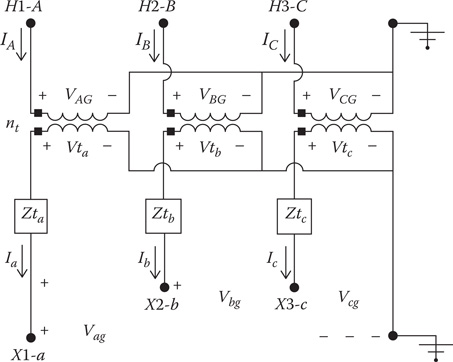
Figure 8.14
Grounded wye–grounded wye connection.

$\begin{array}{l} [\begin{matrix} V_{A G} \\ V_{B G} \\ V_{C G} \end{matrix}] = n_{t} \cdot [\begin{matrix} 1 & 0 & 0 \\ 0 & 1 & 0 \\ 0 & 0 & 1 \end{matrix}] \cdot [\begin{matrix} V_{t}_{_{a g}} \\ V_{t}_{_{b g}} \\ V_{t}_{_{c g}} \end{matrix}] \\ [V_{L G}_{_{A B C}}] = [A V] \cdot [V_{t}_{_{a b c}}] \end{array}$ (8.116)

where

$[A V] = n_{t} \cdot [\begin{matrix} 1 & 0 & 0 \\ 0 & 1 & 0 \\ 0 & 0 & 1 \end{matrix}]$

$\begin{array}{l} [\begin{matrix} I_{A} \\ I_{B} \\ I_{C} \end{matrix}] = \frac{1}{n_{t}} \cdot [\begin{matrix} 1 & 0 & 0 \\ 0 & 1 & 0 \\ 0 & 0 & 1 \end{matrix}] \cdot [\begin{matrix} I_{a} \\ I_{b} \\ I_{c} \end{matrix}] \\ [I_{A B C}] = [A I] \cdot [I_{a b c}] \end{array}$ (8.117)

where

$[A I] = \frac{1}{n_{t}} \cdot [\begin{matrix} 1 & 0 & 0 \\ 0 & 1 & 0 \\ 0 & 0 & 1 \end{matrix}]$

With reference to Figure 8.12, the ideal transformer voltages on the secondary windings can be computed by:

$\begin{array}{l} [\begin{matrix} V_{t}_{_{a}} \\ V_{t}_{_{b}} \\ V_{t}_{_{c}} \end{matrix}] = [\begin{matrix} V_{a g} \\ V_{b g} \\ V_{c g} \end{matrix}] + [\begin{matrix} Z_{t}_{_{a}} & 0 & 0 \\ 0 & Z_{t}_{_{b}} & 0 \\ 0 & 0 & Z_{t}_{_{c}} \end{matrix}] \cdot [\begin{matrix} I_{a} \\ I_{b} \\ I_{c} \end{matrix}] \\ [V_{t}_{_{a b c}}] = [V_{L G}_{_{a b c}}] + [Z_{t}_{_{a b c}}] \cdot [I_{a b c}] \end{array}$ (8.118)

Substitute Equation 8.118 into Equation 8.116:

$\begin{array}{l} [V_{L G}_{_{A B C}}] = [A V] \cdot ([V_{L G}_{_{a b c}}] + [Z_{t}_{_{a b c}}] \cdot [I_{a b c}]) \\ [V_{L G}_{_{A B C}}] = [a_{t}] \cdot [V_{L G}_{_{a b c}}] + [b_{t}] \cdot [I_{a b c}] \end{array}$ (8.119)

Equation 8.119 is the backward sweep equation with the [a_t] and [b_t] matrices defined by:

$[a_{t}] = [A V] = n_{t} \cdot [\begin{matrix} 1 & 0 & 0 \\ 0 & 1 & 0 \\ 0 & 0 & 1 \end{matrix}]$ (8.120)

$[b_{t}] = [A V] . [Z_{t}_{_{a b c}}] = n_{t} \cdot [\begin{matrix} Z_{t}_{_{a}} & 0 & 0 \\ 0 & Z_{t}_{_{b}} & 0 \\ 0 & 0 & Z_{t}_{_{c}} \end{matrix}]$ (8.121)

The primary line currents as a function of the secondary line currents are given by:

$[I_{A B C}] = [d_{t}] \cdot [I_{a b c}]$ (8.122)

where

$[d_{t}] = [A I] = \frac{1}{n_{t}} \cdot [\begin{matrix} 1 & 0 & 0 \\ 0 & 1 & 0 \\ 0 & 0 & 1 \end{matrix}]$

The forward sweep equation is determined solving Equation 8.119 for the secondary line-to-ground voltages:

$\begin{array}{l} [V_{L G}_{_{a b c}}] = {[A V]}^{- 1} \cdot [V_{L G}_{_{A B C}}] - [Z_{t}_{_{a b c}}] \cdot [I_{a b c}] \\ [V_{L G}_{_{a b c}}] = [A_{t}] \cdot [V_{L G}_{_{A B C}}] - [B_{t}] \cdot [I_{a b c}] \end{array}$ (8.123)

where

$\begin{array}{l} [A_{t}] = {[A V]}^{- 1} \\ [B_{t}] = [Z_{t}_{_{a b c}}] \end{array}$

The modeling and analysis of the grounded wye–grounded wye connection does not present any problems. Without the phase shift, there is a direct relationship between the primary and secondary voltages and currents as had been demonstrated in the derivation of the generalized constant matrices.

8.10 The Delta–Delta Connection

The delta–delta connection is primarily used on three-wire delta systems to provide service to a three-phase load or a combination of three-phase and single-phase loads. Three single-phase transformers connected in a delta–delta are shown in Figure 8.15.

The basic “ideal” transformer voltage and current equations as a function of the “turn’s ratio” are:

$n_{t} = \frac{V_{L L}_{_{rated primary}}}{V_{L L}_{_{rated secondary}}}$ (8.124)

$\begin{array}{l} [\begin{matrix} V_{L L}_{_{A B}} \\ V_{L L}_{_{B C}} \\ V_{L L}_{_{C A}} \end{matrix}] = n_{t} \cdot [\begin{matrix} 1 & 0 & 0 \\ 0 & 1 & 0 \\ 0 & 0 & 1 \end{matrix}] \cdot [\begin{matrix} V_{t}_{_{a b}} \\ V_{t}_{_{b c}} \\ V_{t}_{_{c a}} \end{matrix}] \\ [V_{L L}_{_{A B C}}] = [A V] \cdot [V_{t}_{_{a b c}}] \end{array}$ (8.125)

where

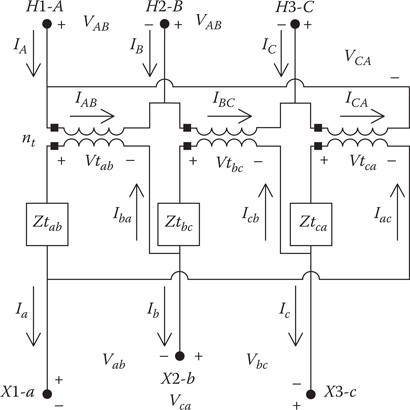
$[A V] = n_{t} \cdot [\begin{matrix} 1 & 0 & 0 \\ 0 & 1 & 0 \\ 0 & 0 & 1 \end{matrix}]$

images

Figure 8.15
Delta–delta connection.

$\begin{array}{l} [\begin{matrix} I_{A B} \\ I_{B C} \\ I_{C A} \end{matrix}] = \frac{1}{n_{t}} \cdot [\begin{matrix} 1 & 0 & 0 \\ 0 & 1 & 0 \\ 0 & 0 & 1 \end{matrix}] \cdot [\begin{matrix} I_{b a} \\ I_{c b} \\ I_{a c} \end{matrix}] \\ [I_{D}_{_{A B C}}] = [A I] \cdot [I_{D}_{_{a b c}}] \end{array}$ (8.126)

where

$[A I] = \frac{1}{n_{t}} \cdot [\begin{matrix} 1 & 0 & 0 \\ 0 & 1 & 0 \\ 0 & 0 & 1 \end{matrix}]$

Solve Equation 8.126 for the secondary-side delta currents:

$[I_{D}_{_{a b c}}] = {[A I]}^{- 1} \cdot [I_{D}_{_{A B C}}]$ (8.127)

The line currents as a function of the delta currents on the source side are given by:

$\begin{array}{l} [\begin{matrix} I_{A} \\ I_{B} \\ I_{C} \end{matrix}] = [\begin{matrix} 1 & 0 & - 1 \\ - 1 & 1 & 0 \\ 0 & - 1 & 1 \end{matrix}] \cdot [\begin{matrix} I_{A B} \\ I_{B C} \\ I_{C A} \end{matrix}] \\ [I_{A B C}] = [D i] \cdot [I_{D}_{_{A B C}}] \end{array}$ (8.128)

where

$[D i] = [\begin{matrix} 1 & 0 & - 1 \\ - 1 & 1 & 0 \\ 0 & - 1 & 1 \end{matrix}]$

Substitute Equation 8.126 into Equation 8.128:

$[I_{A B C}] = [D i] \cdot [A I] \cdot [I_{D}_{_{a b c}}]$ (8.129)

Since [AI]is a diagonal matrix, Equation 8.129 can be rewritten as:

$[I_{A B C}] = [A I] \cdot [D i] \cdot [I_{D}_{_{a b c}}]$ (8.130)

The load-side line currents as a function of the load-side delta currents are:

$\begin{array}{l} [I_{a b c}] = [D i] \cdot [I_{D}_{_{a b c}}] \\ or: [I_{D}_{_{a b c}}] = {[D i]}^{- 1} \cdot [I_{a b c}] \\ even though {[D i]}^{- 1} is singular \end{array}$ (8.131)

Applying Equation 8.131, Equation 8.130 becomes:

$\begin{array}{l} [I_{A B C}] = [A I] \cdot [D i] \cdot {[D i]}^{- 1} \cdot [I_{a b c}] \\ [I_{A B C}] = [A I] \cdot [I_{a b c}] \end{array}$ (8.132)

Turn Equation 8.132 around to solve for the load-side line currents as a function of the source-side line currents:

$[I_{a b c}] = {[A I]}^{- 1} \cdot [I_{A B C}]$ (8.133)

Equations 8.132 and 8.133 merely demonstrate that the line currents on the two sides of the transformer are in phase and differ only by the turn’s ratio of the transformer windings. In the per-unit system, the per-unit line currents on the two sides of the transformer are exactly equal.

The ideal delta voltages on the secondary side as a function of the line-to-line voltages of the delta currents and the transformer impedances are given by:

$[V_{t}_{_{a b c}}] = [V_{L L}_{_{a b c}}] + [Z_{t}_{_{a b c}}] \cdot [I_{D}_{_{a b c}}]$ (8.134)

where

$[Z_{t}_{_{a b c}}] = [\begin{matrix} Z_{t}_{_{a b}} & 0 & 0 \\ 0 & Z_{t}_{_{b c}} & 0 \\ 0 & 0 & Z_{t}_{_{c a}} \end{matrix}]$

Substitute Equation 8.134 into Equation 8.125:

$[V_{L L}_{_{A B C}}] = [A V] \cdot [V_{L L}_{_{a b c}}] + [A V] \cdot [Z_{t}_{_{a b c}}] \cdot [I_{D}_{_{a b c}}]$ (8.135)

Solve Equation 8.135 for the load-side line-to-line voltages:

$[V_{L L}_{_{a b c}}] = {[A V]}^{- 1} \cdot [V_{L L}_{_{A B C}}] - [Z_{t}_{_{a b c}}] \cdot [I_{D}_{_{a b c}}]$ (8.136)

The delta currents [ID_abc] in Equations 8.135 and 8.136 need to be replaced by the secondary line currents [I_abc]. In order to develop the needed relationship, three independent equations are needed. The first two come from applying KCL at two vertices of the delta-connected secondary.

$\begin{array}{l} I_{a} = I_{b a} - I_{a c} \\ I_{b} = I_{c b} - I_{b a} \end{array}$ (8.137)

The third equation comes from recognizing that the sum of the primary line-to-line voltages and therefore the secondary ideal transformer voltages must sum to zero. KVL around the delta windings gives:

$V_{t}_{_{a b}} - Z_{t}_{_{a b}} \cdot I_{b a} + V_{t}_{_{b c}} - Z_{t}_{_{b c}} \cdot I_{c b} + V_{t}_{_{c a}} - Z_{t}_{_{c a}} \cdot I_{a c} = 0$ (8.138)

Replacing the “ideal” delta voltages with the source-side line-to-line voltages:

$\frac{V_{A B}}{n_{t}} + \frac{V_{B C}}{n_{t}} + \frac{V_{C A}}{n_{t}} = Z_{t}_{_{a b}} \cdot I_{b a} + Z_{t}_{_{b c}} \cdot I_{c b} + Z_{t}_{_{c a}} \cdot I_{a c}$ (8.139)

Because the sum of the line-to-line voltages must equal zero (KVL) and the turn’s ratios of the three transformers are equal, Equation 8.139 is simplified to:

$0 = Z_{t}_{_{a}} \cdot I_{b a} + Z_{t}_{_{b}} \cdot I_{c b} + Z_{t}_{_{c}} \cdot I_{a c}$ (8.140)

Note in Equation 8.140 that if the three transformer impedances are equal, then the sum of the delta currents will add to zero, meaning that the zero sequence delta currents will be zero.

Equations 8.137 and 8.140 can be put into matrix form:

$\begin{array}{l} [\begin{matrix} I_{a} \\ I_{b} \\ 0 \end{matrix}] = [\begin{matrix} 1 & 0 & - 1 \\ - 1 & 1 & 0 \\ Z_{t}_{_{a b}} & Z_{t}_{_{b c}} & Z_{t}_{_{c a}} \end{matrix}] \cdot [\begin{matrix} I_{b a} \\ I_{c b} \\ I_{a c} \end{matrix}] \\ [I 0_{a b c}] = [F] \cdot [I_{D}_{_{a b c}}] \end{array}$ (8.141)

where

$\begin{array}{l} [I 0_{a b c}] = [\begin{matrix} I_{a} \\ I_{b} \\ 0 \end{matrix}] \\ [F] = [\begin{matrix} 1 & 0 & - 1 \\ - 1 & 1 & 0 \\ Z_{t}_{_{a b}} & Z_{t}_{_{b c}} & Z_{t}_{_{c a}} \end{matrix}] \end{array}$

Solve Equation 8.141 for the load-side delta currents:

$[I_{D}_{_{a b c}}] = {[F]}^{- 1} \cdot [I 0_{a b c}] = [G] \cdot [I 0_{a b c}]$ (8.142)

where

$[G] = {[F]}^{- 1}$

Writing Equation 8.142 in matrix form gives:

$[\begin{matrix} I_{b a} \\ I_{c b} \\ I_{a c} \end{matrix}] = [\begin{matrix} G_{11} & G_{12} & G_{13} \\ G_{21} & G_{22} & G_{23} \\ G_{31} & G_{32} & G_{33} \end{matrix}] \cdot [\begin{matrix} I_{a} \\ I_{b} \\ 0 \end{matrix}]$ (8.143)

From Equations 8.142 and 8.143, it is seen that the delta currents are a function of the transformer impedances and just the line currents in phases a and b. Equation 8.143 can be modified to include the line current in phase c by setting the last column of the [G] matrix to zeros.

where

$\begin{array}{l} [\begin{matrix} I_{b a} \\ I_{c b} \\ I_{a c} \end{matrix}] = [\begin{matrix} G_{11} & G_{11} & 0 \\ G_{21} & G_{22} & 0 \\ G_{31} & G_{32} & 0 \end{matrix}] \cdot [\begin{matrix} I_{a} \\ I_{b} \\ I_{c} \end{matrix}] \\ [I D_{a b c}] = [G_{1}] \cdot [I_{a b c}] \end{array}$ (8.144)

where

$[G_{1}] = [\begin{matrix} G_{11} & G_{12} & 0 \\ G_{21} & G_{22} & 0 \\ G_{31} & G_{32} & 0 \end{matrix}]$

When the impedances of the transformers are equal, the sum of the delta currents will be zero, meaning that there is no circulating zero sequence current in the delta windings.

Substitute Equation 8.144 into Equation 8.135:

$[V_{L L}_{_{A B C}}] = [A V] \cdot [V_{L L}_{_{a b c}}] + [A V] [Z_{t}_{_{a b c}}] \cdot [G_{1}] \cdot [I_{a b c}]$ (8.145)

The generalized matrices are defined in terms of the line-to-neutral voltages on the two sides of the transformer bank. Equation 8.145 is modified to be in terms of equivalent line-to-neutral voltages.

$\begin{array}{l} [V_{L N}_{_{A B C}}] = [W] \cdot [V_{L L}_{_{A B C}}] \\ [V_{L N}_{_{A B C}}] = [W] [A V] \cdot [D v] \cdot [V_{L N}_{_{a b c}}] + [W] \cdot [Z_{t}_{_{a b c}}] \cdot [G_{1}] \cdot [I_{a b c}] \end{array}$ (8.146)

Equation 8.146 is in the general form:

$[V_{L N}_{_{A B C}}] = [a_{t}] \cdot [V_{L N}_{_{a b c}}] + [b_{t}] \cdot [I_{a b c}]$ (8.147)

where

$\begin{array}{l} [a_{t}] = [W] \cdot [A V] \cdot [D v] \\ [b_{t}] = [A V] [W] \cdot [Z_{t}_{_{a b c}}] \cdot [G_{1}] \end{array}$

Equation 8.133 gives the generalized equation for currents:

$[I_{A B C}] = [A I] \cdot [I_{a b c}] = [d_{t}] \cdot [I_{a b c}]$ (8.148)

where

$[d_{t}] = [A I]$

The forward sweep equations can be derived by modifying Equation 8.136 in terms of equivalent line-to-neutral voltages.

$\begin{array}{l} [V_{L N}_{_{a b c}}] = [W] \cdot [V_{L L}_{_{a b c}}] \\ [V_{L N}_{_{a b c}}] = [W] \cdot {[A V]}^{- 1} \cdot [D v] \cdot [V_{L N}_{_{A B C}}] - [W] \cdot [Z_{t}_{_{a b c}}] \cdot [G_{1}] \cdot [I_{a b c}] \end{array}$ (8.149)

The forward sweep equation is:

$[V_{L N}_{_{a b c}}] = [A_{t}] \cdot [V_{L N}_{_{A B C}}] - [B_{t}] \cdot [I_{a b c}]$ (8.150)

where

$\begin{array}{l} [A_{t}] = [W] \cdot {[A V]}^{- 1} \cdot [D v] \\ [B_{t}] = [W] \cdot [Z_{t}_{_{a b c}}] \cdot [G_{1}] \end{array}$

The forward and backward sweep matrices for the delta–delta connection have been derived. Once again, it has been a long process to get to the final six equations that define the matrices. The derivation provides an excellent exercise in the application of basic transformer theory and circuit theory. Once the matrices have been defined for a particular transformer connection, the analysis of the connection is a relatively simple task. Example 8.8 will demonstrate the analysis of this connection using the generalized matrices.

Example 8.8

Figure 8.16 shows three single-phase transformers in a delta–delta connection serving an unbalanced three-phase load connected in delta. The source voltages at the load are balanced three-phase of 240 V line-to-line.

$[V_{L L}_{_{a b c}}] = [\begin{matrix} 12, 470 \underset{__}{/ 0} \\ 12, 470 \underset{_____}{/ - 120} \\ 12, 470 \underset{_____}{/ 120} \end{matrix}] V$

The loading by phase is:

S_ab =100 kVA at 0.9 lagging power factor

S_bc = S_ca = 50 kVA at 0.8 lagging power factor

The ratings of the transformers are:

Phase A–B: 100 kVA, 12,470–240 V, Z = 0.01 + j0.04 per unit

Phases B–C and C–A: 50 kVA, 12,470–240 V, Z = 0.015 + j0.035 per unit

Determine the following:

The load line-to-line voltages
The secondary line currents
The primary line currents
The load currents
Load voltage unbalance

Before the analysis can start, the transformer impedances must be converted to actual values in ohms and located inside the delta-connected secondary windings.

images

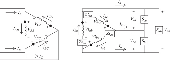
Figure 8.16
Delta–delta bank serving an unbalanced delta-connected load.

Phase a–b transformer:

$Z_{base} = \frac{{0.24}^{2} \cdot 1000}{100} = 0.576 Ω$

$Z_{t}_{_{a b}} = (0.01 + j 0.04) \cdot 0.576 = 0.0058 + j .023 Ω$

Phase b–c and c–a transformers:

$Z_{base} = \frac{{0.24}^{2} \cdot 1000}{50} = 1.152 Ω$

$Z_{t}_{_{b c}} = Z_{t}_{_{c a}} = (0.015 + j 0.035) \cdot 1.152 = 0.0173 + j 0.0403 Ω$

The transformer impedance matrix can now be defined as:

$[Z_{t}_{_{a b c}}] = [\begin{matrix} 0.0058 + j .023 & 0 & 0 \\ 0 & 0.0173 + j .0403 & 0 \\ 0 & 0 & 0.0173 + j .0403 \end{matrix}] Ω$

The turn’s ratio of the transformers is: $n_{t} = \frac{12, 470}{240} = 51.9583$

Define all of the matrices:

$[A V] = n_{t} \cdot [\begin{matrix} 1 & 0 & 0 \\ 0 & 1 & 0 \\ 0 & 0 & 1 \end{matrix}] = [\begin{matrix} 51.9583 & 0 & 0 \\ 0 & 51.9583 & 0 \\ 0 & 0 & 51.9583 \end{matrix}]$

$[A I] = \frac{1}{n_{t}} \cdot [\begin{matrix} 1 & 0 & 0 \\ 0 & 1 & 0 \\ 0 & 0 & 1 \end{matrix}] = [\begin{matrix} 0.0192 & 0 & 0 \\ 0 & 0.0192 & 0 \\ 0 & 0 & 0.0192 \end{matrix}]$

$[F] = [\begin{matrix} 1 & 0 & - 1 \\ - 1 & 1 & 0 \\ 0.0058 + j 0.023 & 0.0173 + j 0.0403 & 0.0173 + j 0.0404 \end{matrix}]$

$[G] = {[F]}^{- 1} = [\begin{matrix} 0.3941 - j 0.0134 & - 0.3941 + j 0.0134 & 3.2581 - j 8.378 \\ 0.3941 - j 0.0134 & 0.6059 + j 0.0134 & 3.2581 - j 8.378 \\ - 0.6059 - j 0.0134 & - 0.3941 + j 0.0134 & 3.2581 - j 8.378 \end{matrix}]$

$[G_{1}] = [\begin{matrix} 0.3941 - j 0.0134 & - 0.3941 + j 0.0134 & 0 \\ 0.3941 - j 0.0134 & 0.6059 + j 0.0134 & 0 \\ - 0.6059 - j 0.0134 & - 0.3941 + j 0.0134 & 0 \end{matrix}]$

$[a_{t}] = [W] \cdot [A V] \cdot [D v] = [\begin{matrix} 34.6489 & - 17.3194 & - 17.3194 \\ - 17.3194 & 34.6489 & - 17.3194 \\ - 17.3194 & - 17.3194 & 34.6489 \end{matrix}]$

$[b_{t}] = [A V] \cdot [W] \cdot [Z_{t}_{_{a b c}}] \cdot [G_{1}] = [\begin{matrix} 0.2166 + j 0.583 & 0.0826 + j 0.1153 & 0 \\ 0.0826 + j 0.1153 & 0.2166 + j 0.583 & 0 \\ - 0.2993 - j 0.6983 & - 0.2993 - j 0.6983 & 0 \end{matrix}]$

$[d_{t}] = [A I] = [\begin{matrix} 0.0192 & 0 & 0 \\ 0 & 0.0192 & 0 \\ 0 & 0 & 0.0192 \end{matrix}]$

$[A_{t}] = [W] \cdot {[A V]}^{- 1} \cdot [D] = [\begin{matrix} 0.0128 & - 0.0064 & - 0.0064 \\ - 0.0064 & 0.0128 & - 0.0064 \\ - 0.0064 & - 0.0064 & 0.0128 \end{matrix}]$

$[B_{t}] = [W] \cdot [Z_{t}_{_{a b c}}] \cdot [G_{1}] = [\begin{matrix} 0.0042 + j 0.0112 & 0.0016 + j 0.0022 & 0 \\ 0.0016 + j 0.0022 & 0.0042 + j 0.0112 & 0 \\ - 0.0058 - j 0.0134 & - 0.0058 - j 0.0134 & 0 \end{matrix}]$

The Mathcad program is modified slightly to account for the delta connections. The modified program is shown in Figure 8.17. The initial conditions are:

$[V_{L L}_{_{A B C}}] = [\begin{matrix} 12470 \underset{_____}{/ 30} \\ 12470 \underset{_____}{/ - 90} \\ 12470 \underset{_____}{/ 1500} \end{matrix}] [Start] = [\begin{matrix} 0 \\ 0 \\ 0 \end{matrix}] T o l = 0.000001 V M = 240$

After six iterations, the results are:

$[{V L L}_{a b c}] = [\begin{matrix} 232.9 \underset{_____}{/ 28.3} \\ 231.0 \underset{_____}{/ - 91.4} \\ 233.1 \underset{_____}{/ 148.9} \end{matrix}]$

$[I_{a b c}] = [\begin{matrix} 540.3 \underset{_____}{/ - 19.5} \\ 593.6 \underset{_____}{/ - 161.5} \\ 372.8 \underset{_____}{/ 81.7} \end{matrix}]$

$[I_{A B C}] = [\begin{matrix} 10.4 \underset{_____}{/ - 19.5} \\ 11.4 \underset{_____}{/ - 161.5} \\ 7.2 \underset{_____}{/ 81.7} \end{matrix}]$

images

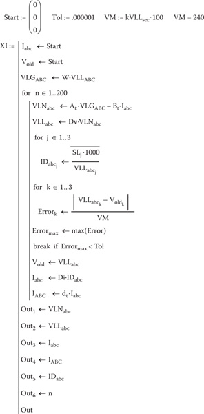
Figure 8.17
Delta–delta Mathcad program.

$[{I D}_{a b c}_{1}] = [\begin{matrix} 429.3 \underset{_____}{/ 2.4} \\ 216.5 \underset{_____}{/ - 128.3} \\ 214.5 \underset{_____}{/ 112.0} \end{matrix}] A$

$V_{u n b a l a n c e} = 0.59 %$

This example demonstrates that a small change in the Mathcad program can be made to represent the delta–delta transformer connection.

8.11 Open Delta–Open Delta

The open delta–open delta transformer connection can be connected in three different ways. Figure 8.18 shows the connection using phase AB and BC.

The relationship between the primary line-to-line voltages and the secondary ideal voltage is given by:

$\begin{array}{l} [\begin{matrix} V_{A B} \\ V_{B C} \\ V_{C A} \end{matrix}] = n_{t} \cdot [\begin{matrix} 1 & 0 & 0 \\ 0 & 1 & 0 \\ - 1 & - 1 & 0 \end{matrix}] \cdot [\begin{matrix} V_{t}_{_{a b}} \\ V_{t}_{_{b c}} \\ V_{t}_{_{c a}} \end{matrix}] \\ [V_{L L}_{_{A B C}}] = [A V] \cdot [V_{t}_{_{a b c}}] \end{array}$ (8.151)

where

$[A V] = n_{t} \cdot [\begin{matrix} 1 & 0 & 0 \\ 0 & 1 & 0 \\ - 1 & - 1 & 0 \end{matrix}]$

The last row of the matrix [AV] is the result that the sum of the line-to-line voltages must be equal to zero.

images

Figure 8.18
Open delta–open delta using phases AB and BC.

The relationship between the secondary and primary line currents is:

$\begin{array}{l} [\begin{matrix} I_{A} \\ I_{B} \\ I_{C} \end{matrix}] = \frac{1}{n_{t}} \cdot [\begin{matrix} 1 & 0 & 0 \\ - 1 & 0 & - 1 \\ 0 & 0 & 1 \end{matrix}] \cdot [\begin{matrix} I_{a} \\ I_{b} \\ I_{c} \end{matrix}] \\ [I_{A B C}] = [A I] \cdot [I_{a b c}] \end{array}$ (8.152)

where

$[A I] = [d_{t}] = \frac{1}{n_{t}} \cdot [\begin{matrix} 1 & 0 & 0 \\ - 1 & 0 & - 1 \\ 0 & 0 & 1 \end{matrix}]$

The ideal secondary voltages are given by:

$\begin{array}{l} V_{t}_{_{a b}} = V_{a b} + Z_{t}_{_{a b}} \cdot I_{a} \\ V_{t}_{_{b c}} = V_{b c} + Z_{t}_{_{b c}} \cdot I_{c} \end{array}$ (8.153)

The primary line-to-line voltages as a function of the secondary line-to-line voltages are given by:

$\begin{array}{l} V_{A B} = n_{t} \cdot V_{t}_{_{a b}} = n_{t} \cdot V_{a b} + n_{t} \cdot Z_{t}_{_{a b}} \cdot I_{a} \\ V_{B C} = n_{t} \cdot V_{t}_{_{b c}} = n_{t} \cdot V_{b c} + n_{t} \cdot Z_{t}_{_{b c}} \cdot I_{c} \end{array}$ (8.154)

The sum of the primary line-to-line voltages must equal zero. Therefore, the voltage V_CA is given by:

$\begin{array}{l} V_{C A} = - (V_{A B} + V_{B C}) = - n_{t} \cdot (V_{a b} + n_{t} \cdot Z_{t}_{_{a b}} \cdot I_{a} + V_{b c} + n_{t} \cdot Z_{t}_{_{b c}} \cdot I_{c}) \\ V_{C A} = - n_{t} \cdot V_{a b} - n_{t} \cdot V_{b c} - n_{t} \cdot Z_{t}_{_{a b}} \cdot I_{a} - n_{t} \cdot Z_{t}_{_{b c}} \cdot I_{c} \end{array}$ (8.155)

Equations 8.154 and 8.155 can be put into matrix form to create the backward sweep voltage equation:

$[V_{L L}_{_{A B C}}] = [A V] \cdot [V_{L L}_{_{a b c}}] + n_{t} \cdot [Z_{t}_{_{a b c}}] \cdot [I_{a b c}]$ (8.156)

where

$[Z_{t}_{_{a b c}}] = [\begin{matrix} Z_{t}_{_{a b}} & 0 & 0 \\ 0 & 0 & Z_{t}_{_{b c}} \\ - Z_{t}_{_{a b}} & 0 & - Z_{t}_{_{b c}} \end{matrix}]$

Equation 8.156 gives the backward sweep equation in terms of line-to-line voltages. In order to convert the equation to equivalent line-to-neutral voltages, the [W] and [D_V] matrices are applied to Equation 8.156.

$\begin{array}{l} [V_{L L}_{_{A B C}}] = [A V] \cdot [V_{L L}_{_{a b c}}] + n_{t} \cdot [Z_{t}_{_{a b c}}] \cdot [I_{a b c}] \\ [V_{L N}_{_{A B C}}] = [W] \cdot [V_{L L}_{_{A B C}}] = [W] \cdot [A V] \cdot [D v] \cdot [V_{L N}_{_{a b c}}] + [W] \cdot n_{t} \cdot [Z_{t}_{_{a b c}}] \cdot [I_{a b c}] \\ [V_{L N}_{_{A B C}}] = [a_{t}] \cdot [V_{L N}_{_{a b c}}] + [b_{t}] \cdot [I_{a b c}] \end{array}$ (8.157)

where

$\begin{array}{l} [a_{t}] = [W] \cdot [A V] \cdot [D v] \\ [b_{t}] = [W] \cdot n_{t} \cdot [Z_{t}_{_{a b c}}] \end{array}$

The forward sweep equation can be derived by defining the ideal voltages as a function of the primary line-to-line voltages:

$\begin{array}{l} [\begin{matrix} V_{t}_{_{a b}} \\ V_{t}_{_{b c}} \\ V_{t}_{_{c a}} \end{matrix}] = \frac{1}{n_{t}} . [\begin{matrix} 1 & 0 & 0 \\ 0 & 1 & 0 \\ - 1 & - 1 & 0 \end{matrix}] \cdot [\begin{matrix} V_{A B} \\ V_{B C} \\ V_{C A} \end{matrix}] \\ [V_{t}_{_{a b c}}] = [B V] \cdot [V_{L L}_{_{A B C}}] \end{array}$ (8.158)

where

$[B V] = \frac{1}{n_{t}} . [\begin{matrix} 1 & 0 & 0 \\ 0 & 1 & 0 \\ - 1 & - 1 & 0 \end{matrix}]$

The ideal secondary voltages as a function of the terminal line-to-line voltages are given by:

$\begin{array}{l} [\begin{matrix} V_{t}_{_{a b}} \\ V_{t}_{_{b c}} \\ V_{t}_{_{c a}} \end{matrix}] = [\begin{matrix} V_{a b} \\ V_{b c} \\ V_{c a} \end{matrix}] + [\begin{matrix} Z_{t}_{_{a b}} & 0 & 0 \\ 0 & 0 & Z_{t}_{_{b c}} \\ - Z_{t}_{_{a b}} & 0 & - Z_{t}_{_{b c}} \end{matrix}] \cdot [\begin{matrix} I_{a} \\ I_{b} \\ I_{c} \end{matrix}] \\ [V_{t}_{_{a b c}}] = [V_{L L}_{_{a b c}}] + [Z_{t}_{_{a b c}}] \cdot [I_{a b c}] \end{array}$ (8.159)

where

$[Z_{t}_{_{a b c}}] = [\begin{matrix} Z_{t}_{_{a b}} & 0 & 0 \\ 0 & 0 & Z_{t}_{_{b c}} \\ - Z_{t}_{_{a b}} & 0 & - Z_{t}_{_{b c}} \end{matrix}]$

Equate Equation 8.158 to Equation 8.159:

$\begin{array}{l} [B V] \cdot [V_{L L}_{_{A B C}}] = [V_{L L}_{_{a b c}}] + [Z_{t}_{_{a b c}}] \cdot [I_{a b c}] \\ [V_{L L}_{_{a b c}}] = [B V] \cdot [V_{L L}_{_{A B C}}] - [Z_{t}_{_{a b c}}] \cdot [I_{a b c}] \end{array}$ (8.160)

Equation 8.160 gives the forward sweep equation in terms of line-to-line voltages. As before, the [W] and [D] matrices are used to convert Equation 8.160 to line-to-neutral voltages as shown in Equation 8.161:

$\begin{array}{l} [V_{L L}_{_{a b c}}] = [B V] \cdot [V_{L L}_{_{A B C}}] - [Z_{t}_{_{a b c}}] \cdot [I_{a b c}] \\ [V_{L N}_{_{a b c}}] = [W] \cdot [V_{L L}_{_{a b c}}] = [W] \cdot [B V] \cdot [D v] \cdot [V_{L N}_{_{A B C}}] - [W] \cdot [Z_{t}_{_{a b c}}] \cdot [I_{a b c}] \\ [V_{L N}_{_{a b c}}] = [A_{t}] \cdot [V_{L N}_{_{A B C}}] - [B_{t}] \cdot [I_{a b c}] \end{array}$ (8.161)

where

$\begin{array}{l} [A_{t}] = [W] \cdot [B V] \cdot [D v] \\ [B_{t}] = [W] \cdot [Z_{t}_{_{a b c}}] \end{array}$

Example 8.9

In Example 8.8, remove the transformer connected between phases C and A. This creates an open delta–open delta transformer bank. This transformer bank serves the same loads as in Example 8.8.

Determine the following:

The load line-to-line load voltages
The secondary line currents
The primary line currents
The load currents
Load voltage unbalance

The exact same program from Example 8.8 is used, since only the values of the matrices change for this connection. After six iterations, the results are:

$[V_{L L}_{_{a b c}}] = [\begin{matrix} 229.0 \underset{_____}{/ 28.5} \\ 248.2 \underset{_____}{/ - 86.9} \\ 255.4 \underset{_____}{/ 147.2} \end{matrix}]$

$[I_{a b c}] = [\begin{matrix} 529.9 \underset{_____}{/ - 17.9} \\ 579.6 \underset{_____}{/ - 161.1} \\ 353.8 \underset{_____}{/ 82.8} \end{matrix}]$

$[I_{A B C}] = [\begin{matrix} 10.2 \underset{_____}{/ - 17.9} \\ 11.2 \underset{_____}{/ - 161.1} \\ 6.8 \underset{_____}{/ 82.8} \end{matrix}]$

$[I_{D}_{_{a b c}}] = [\begin{matrix} 436.7 \underset{_____}{/ 2.7} \\ 201.4 \underset{_____}{/ - 123.8} \\ 195.8 \underset{_____}{/ 110.3} \end{matrix}]$

$V_{unbalance} = 6.2 %$

An inspection of the line-to-line load voltages should raise a question, as two of the three voltages are greater than the no-load voltages of 240 V. Why is there an apparent voltage rise on two of the phases? This can be explained by computing the voltage drops in the secondary circuit:

$\begin{array}{l} v_{a} = Z_{t}_{_{a b}} \cdot I_{a} = 12.6 \underset{_____}{/ 58.0} \\ v_{b} = Z_{t}_{_{b c}} \cdot I_{c} = 15.5 \underset{_____}{/ 149.6} \end{array}$

The ideal voltages are:

$\begin{array}{l} V_{t}_{_{a b}} = 240 \underset{___}{/ 30} \\ V_{t}_{_{b c}} = 240 \underset{_____}{/ - 90} \end{array}$

The terminal voltages are given by:

$\begin{array}{l} V_{a b} = V_{t}_{_{a b}} - v_{a} = 229.0 \underset{_____}{/ 28.5} \\ V_{b c} = V_{t}_{_{b c}} - v_{b} = 248.2 \underset{_____}{/ - 86.9} \\ V_{c a} = - (V_{a b} + V_{b c}) = 255.4 \underset{_____}{/ 147.2} \end{array}$

images

Figure 8.19
Voltage phasor diagram.

Figure 8.19 shows the phasor diagrams (not to scale) for the voltages defined earlier. In the phasor diagram, it is clear that there is a voltage drop on phase ab and then a voltage rise on phase bc. The voltage on ca is also greater than the rated 240 V because the sum of the voltages must add to zero.

It is important that when there is a question about the results of a study, the basic circuit and transformer theory along with a phasor diagram can confirm that the results are correct. This is a good example of when the results should be confirmed. Notice also that the voltage unbalance is much greater for the open delta–open delta than the closed delta–delta connection.

8.12 Thevenin Equivalent Circuit

This chapter has developed the general matrices for the forward and backward sweeps for most standard three-phase transformer connections. In Chapter 10, the section for short-circuit analysis will require the Thevenin equivalent circuit referenced to the secondary terminals of the transformer. This equivalent circuit must take into account the equivalent impedance between the primary terminals of the transformer and the feeder source. Figure 8.20 is a general circuit showing the feeder source down to the secondary bus.

The Thevenin equivalent circuit needs to be determined at the secondary node of the transformer bank. This is basically the same as “referring” the source voltage and the source impedance to the secondary side of the transformer. The desired “Thevenin equivalent circuit” at the transformer secondary node is shown in Figure 8.21.

images

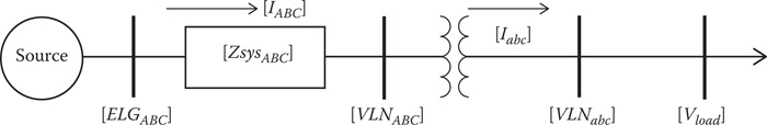
Figure 8.20
Equivalent system.

images

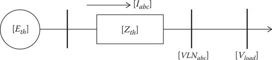
Figure 8.21
The venin equivalent circuit.

A general Thevenin equivalent circuit can be used for all connections defined by the forward and backward sweep matrices.

In Figure 8.18, the primary transformer equivalent line-to-neutral voltages as a function of the source voltages and the equivalent high-side impedance is given by:

$[V_{L N}_{_{A B C}}] = [E_{L N}_{_{A B C}}] - [Z_{sys}_{_{A B C}}] \cdot [I_{A B C}]$ (8.162)

but: [I_abc] = [d_t]⋅[I_abc]

Therefore:

$[V_{L N}_{_{A B C}}] = [E_{L N}_{_{A B C}}] - [Z_{sys}_{_{A B C}}] \cdot [d_{t}] \cdot [I_{a b c}]$ (8.163)

The forward sweep equation gives the secondary line-to-neutral voltages as a function of the primary line-to-neutral voltages.

$[V_{L N}_{_{a b c}}] = [A_{t}] \cdot [V_{L N}_{_{A B C}}] - [B_{t}] \cdot [I_{a b c}]$ (8.164)

Substitute Equation 8.163 into Equation 8.164:

$\begin{array}{l} [V_{L N}_{_{a b c}}] = [A_{t}] . {[E_{L N}_{_{A B C}}] - [Z_{sys}_{_{A B C}}] \cdot [d_{t}] \cdot [I_{a b c}]} - [B_{t}] \cdot [I_{a b c}] \\ [V_{L N}_{_{a b c}}] = [A_{t}] \cdot [E_{L N}_{_{A B C}}] - ([A_{t}] \cdot [Z_{sys}_{_{A B C}}] \cdot [d_{t}] + [B_{t}]) \cdot [I_{a b c}] \\ [V_{L N}_{_{a b c}}] = [E_{t h}] - [Z_{t h}] \cdot [I_{a b c}] \end{array}$ (8.165)

where

$\begin{array}{l} [E_{t h}] = [A_{t}] \cdot [E_{L N}_{_{A B C}}] \\ [Z_{t h}] = ([A_{t}] \cdot [Z_{sys}_{_{A B C}}] \cdot [d_{t}] + [B_{t}]) \end{array}$

The definitions of the Thevenin equivalent voltages and impedances as given in Equation 8.165 are general and can be used for all transformer connections. Example 8.5 is used to demonstrate the computation and application of the Thevenin equivalent circuit.

Example 8.10

The delta–grounded wye transformer bank in Example 8.2 is connected to a balanced three-phase source of 115 kV through a 5-mile section of a four-wire three-phase line as shown in Figure 8.20. The phase impedance matrix for the 5-mile long 115 kV line is given by:

$[Z_{sys}_{_{A B C}}] = [\begin{matrix} 2.2040 + j 5.6740 & 0.6415 + j 2.2730 & 0.6415 + j 1.7850 \\ 0.6415 + j 2.2730 & 2.1430 + j 5.8920 & 0.6130 + j 1.9750 \\ 0.6415 + j 1.7850 & 0.6130 + j 1.9750 & 2.2430 + j 5.8920 \end{matrix}]$

For the unbalanced load in Example 8.2 using a Mathcad program, the load line-to-neutral voltages and secondary and primary currents are computed as:

$\begin{array}{l} [V_{load}] = [\begin{matrix} 6477.3 \underset{_____}{/ - 66.7} \\ 6764.6 \underset{_____}{/ 176.1} \\ 6691.9 \underset{_____}{/ 53.8} \end{matrix}] \\ [I_{a b c}] = [\begin{matrix} 262.5 \underset{_____}{/ - 92.6} \\ 177.4 \underset{_____}{/ 144.3} \\ 224.2 \underset{_____}{/ 35.6} \end{matrix}] \\ [I_{A B C}] = [\begin{matrix} 24.3 \underset{_____}{/ - 70.1} \\ 20.5 \underset{_____}{/ - 175.2} \\ 27.4 \underset{_____}{/ 63.7} \end{matrix}] \end{array}$

The Thevenin equivalent voltages and impedances referred to the secondary terminals of the transformer bank are:

$[E_{t h}_{_{a b c}}] = [A_{t}] \cdot [E_{L N}_{_{A B C}}] = [\begin{matrix} 7200 \underset{_____}{/ - 60} \\ 7200 \underset{_____}{/ 180} \\ 7200 \underset{_____}{/ 60} \end{matrix}] V$

$[Z_{t h}_{_{a b c}}] = [A_{t}] \cdot [Z_{sys}_{_{A B C}}] \cdot [d_{t}] + [B_{t}]$

$[Z_{t h}_{_{a b c}}] = [\begin{matrix} 0.2328 + j 2.6388 & - 0.0012 - j 0.0024 & - 0.0012 - 0.0030 \\ - 0.0012 - j 0.0024 & 0.2328 + j 2.6379 & - 0.0012 - j 0.0020 \\ - 0.0012 - 0.0030 & - 0.0012 - j 0.0020 & 0.2328 + j 2.6384 \end{matrix}] Ω$

The Thevenin equivalent circuit for this case is shown in Figure 8.18. It is always good to confirm the Thevenin equivalent circuit by using the solved-for-load currents and then the Thevenin equivalent circuit to compute the load voltage.

$\begin{array}{l} [V_{load}] = [E_{t h}_{_{a b c}}] - [(Z_{t h}_{_{a b c}} + Z_{line}_{_{a b c}})] \cdot [I_{a b c}] \\ [V_{load}] = [\begin{matrix} 6477.3 \underset{_____}{/ - 66.7} \\ 6464.6 \underset{_____}{/ 176.1} \\ 6691.9 \underset{_____}{/ 53.8} \end{matrix}] \end{array}$

The Mathcad program was modified to match the equivalent system in Figure 8.18. The load voltages and load currents were computed. This example is intended to demonstrate that it is possible to compute the Thevenin equivalent circuit at the secondary terminals of the transformer bank. The example shows that using the Thevenin equivalent circuit and the original secondary line currents, the original equivalent line-to-neutral load voltages are computed. The major application of the Thevenin equivalent circuit will be in the short-circuit analysis of a distribution that will be developed in Chapter 10.

8.13 Summary

In this chapter, the forward and backward sweep matrices have been developed for seven common three-phase transformer bank connections. For unbalanced transformer connections, the derivations were limited to just one of at least three ways that the primary phases could be connected to the transformer bank. The methods in the derivation of these transformer banks can be extended to all possible phasing.

One of the major features of the chapter has been to demonstrate how the forward and backward sweep technique (ladder) is used to analyze the operating characteristics of the transformer banks. Several Mathcad programs were used in the examples to demonstrate how the analysis is mostly independent of the transformer connection by using the derived matrices. This approach was first demonstrated with the line models and then continued to the voltage regulators and now the transformer connections. In Chapter 10, the analysis of a total distribution feeder will be developed using the forward and backward sweep matrices for all possible system components.

Many of the examples demonstrated the use of a Mathcad program for the analysis. An extension of this is the use of the student version of the WindMil distribution analysis program that can be downloaded as explained in the Preface of this text. When the program is downloaded, a “User’s Manual” will be included. The User’s Manual serves two purposes:

A tutorial on how to get started using WindMil for the first-time user
Included will be the WindMil systems for many of the examples in this and other chapters.

It is highly encouraged that the program and manual be downloaded.

Problems

8.1 A three-phase substation transformer is connected delta–grounded wye and rated:

5000 kVA, 115 kV delta—12.47 kV grounded wye, Z = 1.0 + j7.5%

The transformer serves an unbalanced load of:

Phase a: 1384.5 kVA, 89.2% lagging power factor at 6922.5/−33.1 V
Phase b: 1691.2 kVA, 80.2% lagging power factor at 6776.8/−153.4 V
Phase c: 1563.0 kVA, unity power factor at 7104.7/85.9 V
1. Determine the forward and backward sweep matrices for the transformer.
2. Compute the primary equivalent line-to-neutral voltages.
3. Compute the primary line-to-line voltages.
4. Compute the primary line currents.
5. Compute the currents flowing in the high-side delta windings.
6. Compute the real power loss in the transformer for this load condition.

8.2 Write a simple Mathcad or MATLAB^® program using the ladder technique to solve for the load line-to-ground voltages and line currents in the bank of 8.1 when the source voltages are balanced three-phase of 115 kV line-to-line.

8.3 Create the system in WindMil for Problem 8.2.

8.4 Three single-phase transformers are connected in delta–grounded wye serving an unbalanced load. The ratings of three transformers are:

Phase A–B: 100 kVA, 12,470—120 V, Z = 1.3 + j1.7%
Phase B–C: 50 kVA, 12,470—120 V, Z = 1.1 + j1.4%
Phase C–A: same as Phase B–C transformer

The unbalanced loads are:

Phase a: 40 kVA, 0.8 lagging power factor at V = 117.5/ − 32.5 V
Phase b: 85 kVA, 0.95 lagging power factor at V = 115.7/ − 147.3 V
Phase c: 50 kVA, 0.8 lagging power factor at V = 117.0/95.3 V
1. Determine the forward and backward sweep matrices for this connection.
2. Compute the load currents.
3. Compute the primary line-to-neutral voltages.
4. Compute the primary line-to-line voltages.
5. Compute the primary currents.
6. Compute the currents in the delta primary windings.
7. Compute the transformer bank real power loss.

8.5 For the same load and transformers in Problem 8.4, assume that the primary voltages on the transformer bank are balanced three-phase of 12,470 V line-to-line. Write a Mathcad or MATLAB^® program to compute the load line-to-ground voltages and the secondary line currents.

8.6 For the transformer connection and loads in Problem 8.4, build the system in WindMil.

8.7 The three single-phase transformers in Problem 8.4 are serving an unbalanced constant impedance load of:

Phase a: 0.32 + j0.14 Ω
Phase b: 0.21 + j0.08 Ω
Phase c: 0.28 + j0.12 Ω

The transformers are connected to a balanced 12.47 kV source.

Determine the load currents.
Determine the load voltages.
Compute the complex power of each load.
Compute the primary currents.
Compute the operating kVA of each transformer.

8.8 Solve Problem 8.7 using WindMil.

8.9 A three-phase transformer is connected wye–delta and rated as:

500 kVA, 4160—240 V, Z = 1.1 + j3.0%

The primary neutral is ungrounded. The transformer is serving a balanced load of 480 kW with balanced voltages of 235 V line-to-line and a lagging power factor of 0.9.

Compute the secondary line currents.
Compute the primary line currents.
Compute the currents flowing in the secondary delta windings.
Compute the real power loss in the transformer for this load.

8.10 The transformer in Problem 8.9 is serving an unbalanced delta load of:

S_ab = 150 kVA, 0.95 lagging power factor
S_bc = 125 kVA, 0.90 lagging power factor
S_ca = 160 kVA, 0.8 lagging power factor

The transformer bank is connected to a balanced three-phase source of 4160 V line-to-line.

Compute the forward and backward sweep matrices for the transformer bank.
Compute the load equivalent line-to-neutral and line-to-line voltages.
Compute the secondary line currents.
Compute the load currents.
Compute the primary line currents.
Compute the operating kVA of each transformer winding.
Compute the load voltage unbalance.

8.11 Three single-phase transformers are connected in an ungrounded wye–delta connection and serving an unbalanced delta-connected load. The transformers are rated:

Phase A: 15 kVA, 2400–240 V, Z = 1.3 + j1.0%
Phase B: 25 kVA, 2400–240 V, Z = 1.1 + j1.1%
Phase C: Same as phase A transformer

The transformers are connected to a balanced source of 4.16 kV line-to-line. The primary currents entering the transformer are:

I_A = 4.60 A, 0.95 lagging power factor
I_B = 6.92 A, 0.88 lagging power factor
I_C = 5.37 A, 0.69 lagging power factor
1. Determine the primary line-to-neutral voltages. Select V _AB as reference.
2. Determine the line currents entering the delta-connected load.
3. Determine the line-to-line voltages at the load.
4. Determine the operating kVA of each transformer.
5. Is it possible to determine the load currents in the delta-connected load? If so, do it. If not, why not?

8.12 The three transformers in Problem 8.11 are serving an unbalanced delta-connected load of:

S_ab = 10 kVA, 0.95 lagging power factor
S_bc = 20 kVA, 0.90 lagging power factor
S_ca = 15 kVA, 0.8 lagging power factor

The transformers are connected to a balance 4160 line-to-line voltage source. Determine the load voltages, and the primary and secondary line currents for the following transformer connections:

Ungrounded wye–delta connection
Grounded wye–delta connection
Open wye–open delta connection where the transformer connected to phase C has been removed

8.13 Three single-phase transformers are connected in grounded wye–grounded wye and serving an unbalanced constant impedance load. The transformer bank is connected to a balanced three-phase 12.47 line-to-line voltage source. The transformers are rated:

Phase A: 100 kVA, 7200–120 V, Z = 0.9 + j1.8%
Phase B and Phase C: 37.5 kVA, 7200–120 V, Z = 1.1 + j1.4 %

The constant impedance loads are:

Phase a: 0.14 + j0.08 Ω
Phase b: 0.40 + j0.14 Ω
Phase c: 0.50 + j0.20 Ω
1. Compute the generalized matrices for this transformer bank.
2. Determine the load currents.
3. Determine the load voltages.
4. Determine the kVA and power factor of each load.
5. Determine the primary line currents.
6. Determine the operating kVA of each transformer.

8.14 Three single-phase transformers are connected in delta–delta and are serving a balanced three-phase motor rated 150 kVA, 0.8 lagging power factor and a single-phase lighting load of 25 kVA, 0.95 lagging power factor connected across phases a–c. The transformers are rated:

Phase A–B: 75 kVA, 4800–240 V, Z = 1.0 + j1.5%
Phase B–C: 50 kVA, 4800–240 V, Z = 1.1 + j1.4%
Phase C–A: same as Phase B–C

The load voltages are balanced three-phase of 240 V line-to-line.

Determine the forward and backward sweep matrices.
Compute the motor input currents.
Compute the single-phase lighting load current.
Compute the primary line currents.
Compute the primary line-to-line voltages.
Compute the currents flowing in the primary and secondary delta windings.

8.15 In Problem 8.14, the transformers on phases A–B and B–C are connected in an open delta–open delta connection and serving an unbalanced three-phase load of:

Phase a–b: 50 kVA at 0.9 lagging power factor
Phase b–c: 15 kVA at 0.85 lagging power factor
Phase c–a: 25 kVA at 0.95 lagging power factor

The source line-to-line voltages are balanced at 4800 V line-to-line. Determine:

The load line-to-line voltages
The load currents
The secondary line currents
The primary line currents

WindMil Assignment

Use System 4 to build this new System 5. A 5000 kVA delta–grounded wye substation transformer is to be connected between the source and Node 1. The voltages for the transformer are 115 kV delta to 12.47 kV grounded wye. The impedance of this transformer is 8.06% with an X/R ratio 8. By installing this substation transformer, be sure to modify the source so that it is 115,000 V rather than the 12.47 V. Follow the steps in the User’s Manual on how to install the substation transformer.

When the transformer has been connected, run Voltage Drop.
What are the node voltages at Node 2?
What taps has the regulator gone to?
Why did the taps increase when the transformer was added to the system?

..................Content has been hidden....................

You can't read the all page of ebook, please click here login for view all page.

Table of Contents for
8. Three-Phase Transformer Models