In one sense, this section belongs in Chapter 6 or Chapter 7, because in many applications outer joins are as common as inner joins. Indeed, those chapters already cover some of the issues surrounding outer joins. However, some of the questions about outer joins are logically removed from the rest of the tuning problem, and the answers to these questions are clearer if you understand the arguments of Chapter 8. Therefore, I complete the discussion of outer joins here.

Outer joins are notorious for creating performance problems, but they do not have to be a problem when handled correctly. For the most part, the perceived performance problems with outer joins are simply myths, based on either misunderstanding or problems that were fixed long ago. Properly implemented, outer joins are essentially as efficient to execute as inner joins. What’s more, in manual optimization problems, they are actually easier to handle than inner joins.

I already discussed several special issues with outer joins in Chapter 7, under sections named accordingly:

These cases all require special measures already described in Chapter 7. Here, I extend the rules given in Chapter 7 to further optimize the simplest, most common case: simple, unfiltered, downward outer joins to tables, either nodes that are leaf nodes of the query diagram or nodes that lead to further outer joins. Figure 9-1 illustrates this case with 16 outer joins.

Figure 9-1. A query with 16 unfiltered outer joins

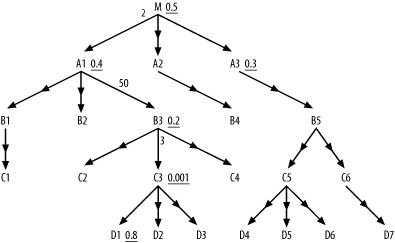
I call these unfiltered, downward outer joins to simple tables normal outer joins. Normal outer joins have a special and useful property, from the point of view of optimization:

This property makes consideration of normal outer joins especially simple; normal outer joins have no effect at all on the running rowcount (the number of rows reached at any point in the join order). Therefore, they are irrelevant to the optimization of the rest of the query. The main justification for performing downward joins before upward joins does not apply; normal outer joins, unlike inner joins, cannot reduce the rowcount going into later, more expensive upward joins. Since they have no effect on the rest of the optimization problem, you should simply choose a point in the join order where the cost of the normal outer join itself is minimum. This turns out to be the point where the running rowcount is minimum, after the first point where the outer-joined table is reachable through the join tree.

Example

These steps require some elaboration. To apply Steps 1 and 2 to Figure 9-1, consider Figure 9-2.

Figure 9-2. The inner query diagram for the earlier query

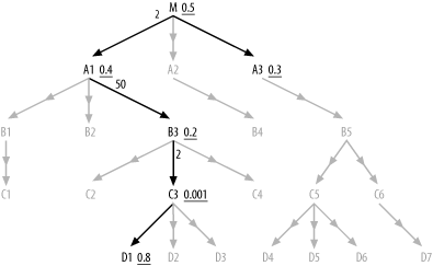
The initially complex-looking 22-way join is reduced in the inner query diagram in black to a simple 6-way join, and it’s an easy optimization problem to find the best inner-join order of (C3, D1, B3, A1, M, A3).

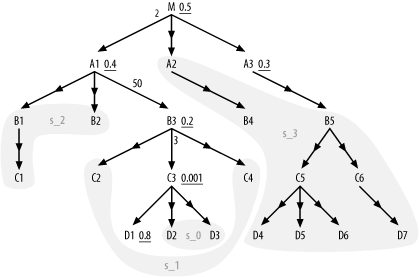
Now, consider Step 3. The driving table is C3, so the subset s_0 contains any normal outer-joined tables reachable strictly through downward joins hanging below C3, which would be the set {D2, D3}. The first upward join is to B3, so s_1 is {C2, C4}, the set of nodes (excluding s_0 nodes) reachable through downward joins from B3. The second upward join is to A1, so s_2 is {B1, B2, C1}. The final upward join is to M, so s_3 holds the rest of the normal outer-joined tables: {A2, B4, B5, C5, C6, D4, D5, D6, D7}. Figure 9-3 shows this division of the outer-joined tables into subsets.

Figure 9-3. The outer-joined-table subsets for the earlier query

Now, consider Step 4. Since you need only comparative (or relative) running rowcounts, let the initial number of rows in C3 be whatever it would need to be to make r_0 a convenient round number—say, 10. From there, work out the list of values for r_n:

r_0: 10

Arbitrary, chosen to simplify the math.

r_1: 6 (r_0 x 3 x 0.2)

The numbers 3 and 0.2 come from the detail join ratio for the join into B3 and the product of all filter ratios picked up before the next upward join. You would also adjust the rowcounts by master join ratios less than 1.0, if there were any, but the example has only the usual master join ratios assumed to be 1.0. (Since there are no filtered nodes below B3 reached after the join to B3, the only applicable filter is the filter on B3 itself, with a filter ratio of 0.2.)

r_2: 120 (r_1 x 50 x 0.4)

The numbers 50 and 0.4 come from the detail join ratio for the join into A1 and the product of all filter ratios picked up before the next upward join. (Since there are no filtered nodes below A1 reached after the join to A1, the only applicable filter is the filter on A1 itself, with a filter ratio of 0.4.)

r_3: 36 (r_2 x 2 x 0.15)

The numbers 2 and 0.15 come from the detail join ratio for the join into M and the product of all remaining filter ratios. (Since there is one filtered node reached after the join to M, A3, the product of all remaining filter ratios is the product of the filter ratio on M (0.5) and the filter ratio on A3 (0.3): 0.5 x 0.3=0.15.)

Finally, apply Step 5. The minimum for all relative rowcounts is r_1, so the subsets s_0 and s_1, which are eligible to join before the query reaches A1, should both join at that point in the join order just before the join to A1. The minimum after that point is r_3, so the subsets s_2 and s_3 should both join at the end of the join order. The only further restriction is that the subsets join from the top down, so that lower tables are reached through the join tree. For example, you cannot join to C1 before you join to B1, nor to D7 before joining to both B5 and C6. Since I have labeled master tables by level, Ds below Cs, Cs below Bs, Bs below As, you can assure top-down joins by just putting each subset in alphabetical order. For example, a complete join order, consistent with the requirements, would be: (C3, D1, B3, {D2, D3}, {C2, C4}, A1, M, A3, {B1, B2, C1}, {A2, B4, B5, C5, C6, D4, D5, D6, D7}), where curly brackets are left in place to show the subsets.

The method I’ve explained so far points you to the best join order for a robust execution plan that assumes you can reach rows in the driving table efficiently and that you have all the indexes you need on the join keys. Occasionally, you can improve on even this nominal best execution plan with an index that combines a join key and one or more filter columns. The problem in Figure 9-4 illustrates the case in which this opportunity arises.

Figure 9-4. A simple three-way join

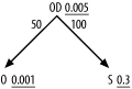
The standard robust plan, following the heuristics of Chapter 6, drives from O with nested loops to the index on OD’s foreign key that points to O. After reaching the table OD, the database discards 99.5% of the rows because they fail to meet the highly selective filter on OD. Then, the database drives to S on its primary-key index and discards 70% of the remaining rows, after reading the table S, because they fail to meet the filter condition on S. In all, this is not a bad execution plan, and it might easily be fast enough if the rowcount of OD and the performance requirements are not too high.

However, it turns out that you can do still better if you enable indexes that are perfect for this query. To make the problem more concrete, assume that Figure 9-4 comes from the following query:

SELECT ... FROM Shipments S, Order_Details OD, Orders O
WHERE O.Order_ID=OD.Order_ID
  AND OD.Shipment_ID=S.Shipment_ID
  AND O.Customer_ID=:1
  AND OD.Product_ID=:2
  AND S.Shipment_Date>:3

Assuming around 1,000 customers, 200 products, and a date for :3 about 30% of the way back to the beginning of the shipment records, the filter ratios shown in the diagram follow. To make the problem even more concrete, assume that the rowcount of Order_Details is 10,000,000. Given the detail join ratio from Orders to Order_Details, the rowcount of Orders must be 200,000, so you would expect to read 200 Orders rows, which would join to 10,000 Order_Details rows. After discarding Order_Details with the wrong Product_IDs, 50 rows would remain in the running rowcount. These would join to 50 rows of Shipments, and 15 rows would remain after discarding the earlier shipments.

Where is the big cost in this execution plan? Clearly, the costs on Orders and Shipments and their indexes are minor, with so few rows read from these tables. The reads to the index on Order_Details(Order_ID) would be 200 range scans, each covering 50 rows. Each of these range scans would walk down a three-deep index and usually touch one leaf block for each range scan for about three logical I/Os per range scan. In all, this would represent about 600 fairly well-cached logical I/Os to the index. Only the Order_Details table itself sees many logical I/Os, 10,000 in all, and that table is large enough that many of those reads will likely also trigger physical I/O. How can you do better?

The trick is to pick up the filter condition on Order_Details before you even reach the table, while still in the index. If you replace the index on Order_Details(Order_ID) with a new index on Order_Details(Order_ID, Product_ID), the 200 range scans of 50 rows each become 200 range scans of an average of just a half row each.

With this new index, you would read only the 50 Order_Details rows that you actually need, a 200-fold savings on physical and logical I/O related to that table. Because Order_Details was the only object in the query to see a significant volume of I/O, this change that I’ve just described would yield roughly a 50-fold improvement in performance of the whole query, assuming much better caching on the other, smaller objects.

So, why did I wait until Chapter 9 to describe such a seemingly huge optimization opportunity? Through most of this book, I have implied the objective of finding the best execution plan, a priori, regardless of what indexes the database has at the time. However, behind this idealization, reality looms: many indexes that are customized to optimize individual, uncommon queries will cost more than they help. While an index that covers both a foreign key and a filter condition will speed the example query, it will slow every insert and delete and many updates when they change the indexed columns. The effect of a single new index on any given insert is minor. However, spread across all inserts and added to the effects of many other custom indexes, a proliferation of indexes can easily do more harm than good.

Consider yet another optimization for the same query. Node S, like OD, is reached through a join key and also has a filter condition. What if you created an index on Shipments(Shipment_ID, Shipment_Date) to avoid unnecessary reads to the Shipments table? Reads to that table would drop 70%, but that is only a savings of 35 logical I/Os and perhaps one or two physical I/Os, which would quite likely not be enough to even notice. In real-world queries, such miniscule improvements with custom indexes that combine join keys and filter conditions are far more common than opportunities for major improvement.

When you find that an index is missing on some foreign key that is necessary to enable a robust plan with the best join order, it is fair to guess that the same foreign-key index will be useful to a whole family of queries. However, combinations of foreign keys and filter conditions are much more likely to be unique to a single query, and the extra benefit of the added filter column is often minor, even within that query.

Consider both the execution frequency of the query you are tuning and the magnitude of the tuning opportunity. If the summed savings in runtime, across the whole application, is an hour or more per day, don’t hesitate to introduce a custom index that might benefit only that single query. If the savings in runtime is less, consider whether the savings affect online performance or just batch load, and consider whether a custom index will do more harm than good. The cases in which it is most likely to do good look most like my contrived example:

When you find a large opportunity for savings on a query that is responsible for much of the database load, these combined key/filter indexes are a valuable tool; just use the tool with caution.

The approach this book has taken so far is to find optimum robust plans as if all driving-table filter conditions and all necessary join keys were already indexed. The implication is that, whenever you find that these optimum plans require an index you don’t already have, you should create it and generate statistics for it so that the optimizer knows its selectivity. If you are tuning only the most important SQL—SQL that contributes (or will contribute) significantly to the load and the perceived performance (from the perspective of the end user) of a real production system—any index you create by following this method will likely be well justified. Cary Millsap’s book Optimizing Oracle Performance (O’Reilly), which I heartily recommend, provides a method for finding the most important SQL to tune.

Unfortunately, you must often tune SQL without much knowledge of its significance to overall production performance and load, especially early in the development process, when you have only tiny data volumes to experiment with and do not yet know the future end users’ patterns of use.

To estimate how important a SQL statement will be to overall load and performance, ask the following questions:

Estimate weekly lost productivity for online delays by using the length of each delay times the frequency of the task per end user times the number of end users. Summed delays of days per week add up to serious lost money. Summed delays of a couple of minutes per week amount to less than you might save by buying an extra coffee maker to save employees steps during coffee breaks; don’t get carried away going after the little stuff!

Consider overriding external effects too. For example, online delays for a live customer-support application that cause customers to find a new vendor can be disproportionately expensive! Similarly, batch delays that trigger penalties for missed deadlines might carry huge costs. When SQL delays are costly and the improvement for adding a new index is significant, don’t hesitate to add the index. Otherwise, consider the trade offs.

The method so far generally assumes that you are tuning queries against large tables, since these dominate the set of SQL that needs tuning. For such queries, especially when they are online queries, you can generally count on finding at least one selective filter that leads to an attractive driving table. Occasionally, especially for large batch queries and online queries of small tables, you will tune unfiltered joins—joins of whole tables without restriction. For example, consider Figure 9-5.

Figure 9-5. An unfiltered three-way join

How do you optimize such a query, with no guidance based on filter selectivities? For nested-loops plans, it hardly matters which join order you choose, as long as you follow the join tree. However, these are precisely the queries that most reward hash joins, or sort-merge joins when hash joins are unavailable. Assuming hash joins are available, the database should read all three tables with full table scans and should hash the smaller tables, A1 and A2, caching these hashed tables in memory if possible. Then, during the single pass through the largest table, M, each hashed row is rapidly matched with the in-memory matching hashed rows of A1 and A2. The cost of the query, ideally, is roughly the cost of the three full table scans. The database can’t do better than that, even theoretically, given that you need all the rows from all three tables. Cost-based optimizers are generally good at finding optimum plans for queries such as these, without manual help.

When either A1 or A2 is too large to cache in memory, consider the more robust nested-loops plan driving from table M, and check how much slower it turns out to be. Indexed lookups, one row at a time, will likely be much slower, but they will eventually succeed, while the hash join runs the risk of exhausting temporary disk space if A1 or A2 is too big to hold in memory.

So far, I’ve described strategies for solving what I would call pure SQL tuning problems, where the text of a slow query constitutes essentially the whole problem statement and where you can tune that query out of context with the rest of the application. The following narrowly defined performance problem statement illustrates the boundaries of the problem I’ve attacked so far:

Assuming the predefined target runtime is set rationally according to real business needs, there are four basic ways that this problem can be unsolvable:

In this section, I describe how to recognize each type of problem. In Chapter 10, I will discuss solving these “unsolvable” problems by stepping outside the box that the too-narrow problem statement imposes.

The first problem type is self-explanatory: the target is way lower than an end user should care about. The explanation turns out to be that a given end-user action or batch process requires the query to run hundreds or even millions of times to perform what, to the end user, is a single task.

The second and third problem types are easy to recognize in a query diagram. Like Figure 9-5, the query, which reads at least one large table, turns out to have no filters or only a couple of weakly selective filters. If you have no aggregation (no GROUP BY, for example), you have the second problem. When you test the best nested-loops plan you can find, with any row-ordering steps removed so you can see rows before sorting, you discover that the query returns rows at a very high rate but returns so many rows that it runs interminably. The third problem, with a GROUP BY or other aggregation, looks just like the second problem type, but with the addition of aggregation.

The fourth problem type is the subtlest. A query diagram with at least one large table has several semiselective filters spread throughout a query diagram, often with subqueries, in such a way that large fractions of one or more large tables must be read before you can reach enough filters to reduce the rowcount to something moderate. This case might sound like it should be quite common, but it actually turns out to be rare; I’ve run into it probably less than once a year, on average.