
CHAPTER 13
Blind Waveform Estimation
Sensor arrays are often used in practice to separate and estimate the waveforms of superimposed signals that share similar frequency spectra but have different spatial structure. Source waveform recovery is traditionally a data communication problem, but the signal-processing techniques developed in this field also have a number of practical radar-related applications. For example, passive radar systems require a “clean copy” of the waveform transmitted by an uncooperative source to perform effective matched filtering. Such systems often receive signals from an emitter of opportunity that are contaminated by multipath arrivals and interference from independent sources. The ability to accurately estimate the signal emitted by an unknown source in the presence of multipath and other sources is not only relevant for passive radar, but is also of interest to active radar systems for interference cancelation.
In many problems of practical interest, the interfering signals do not originate from independent sources radiating on the same frequency channel, but rather arise from a single source due to multipath propagation. This gives rise to a resultant signal that is an additive mixture of amplitude-scaled, time-delayed, and possibly Doppler-shifted versions of the source waveform, which are typically incident from different directions of arrival (DOAs). In real-world environments, multipath propagation from source to receiver often occurs due to diffuse scattering from spatially extended regions of an irregular medium as opposed to ideal specular reflection. This scenario is often encountered in mobile communications, underwater acoustics, and radar systems, for example.
In particular, HF skywave signals usually consist of a relatively small number of dominant multipath components or “modes” that propagate from source to receiver along distinct paths. Each signal mode is in turn composed of many locally scattered “rays” that are clustered in some manner about the nominal mode propagation path. This phenomenon, often referred to as “micro-multipath,” gives each propagating mode its fine structure, and is a feature of so-called doubly-spread channels. The large-scale delay, Doppler, and DOA spread of the channel is due to the well-separated nominal paths of the dominant modes, while on a smaller scale, the spread is also due to the continuum of diffusely scattered rays distributed about each of these nominal paths.
Mutual interference among the different propagation modes may cause significant frequency-selective fading or signal envelope distortions at a single receiver output. This can significantly degrade or even impair the performance of systems that rely on accurate source-waveform estimation. The ability to separate the individual modes by spatial filtering in a narrowband single-input multiple-output (SIMO) system not only isolates the output of one or more useable paths for high fidelity waveform estimation, but may also enable the various signal modes to be combined constructively to benefit from the additional energy that each path provides. The waveform estimation problem may be generalized to multiple sources by considering a multiple-input multiple-output (MIMO) system. In this case, it is necessary to separate the different sources as well as the multipath components of each source for effective waveform estimation.
However, neither the propagation channel characteristics nor the signal properties may be known in practice. Moreover, parametric models that can accurately describe the received signal wavefronts may not be available due to environmental and instrumental uncertainties, including diffuse multipath scattering and array calibration errors, for example. The lack of a priori knowledge regarding both the source signal(s) and propagation channel(s) poses a major challenge for the task at hand. This situation calls for processing techniques that can recover the source waveforms from the received signal mixture in a strictly blind manner.
This chapter discusses blind waveform estimation techniques based on relatively mild assumptions regarding the source signal(s), propagation channel(s), and sensor array. Specifically, a new technique referred to as the Generalized Estimation of Multipath Signals (GEMS) algorithm is introduced. The ability of GEMS to estimate arbitrarily modulated source waveforms in narrowband finite-impulse-response (FIR) SIMO and MIMO systems is experimentally demonstrated and compared against benchmark approaches.
The first section formulates the problem by describing the data model, processing objectives, and main assumptions. The second section explains the relationship between existing blind signal-processing approaches and the specific problem considered to provide motivation for the GEMS technique. The third section introduces the GEMS algorithm and compares its computational complexity with a benchmark approach. The remaining sections present experimental results to illustrate the potential applications of GEMS for blind source waveform and propagation channel estimation in practical HF systems.
13.1 Problem Formulation
Figure 13.1 conceptually illustrates the problem considered. On the left, a number of independent sources are assumed to emit narrowband waveforms with overlapping power spectral densities. These waveforms propagate via different multipath channels before being received by a sensor array in the far-field. Multipath is due to a relatively small number of dominant signal modes, each being composed of possibly a large number of diffusely scattered rays that superimpose to produce distorted (non-planar) wavefronts with path-dependent “crinkles.”
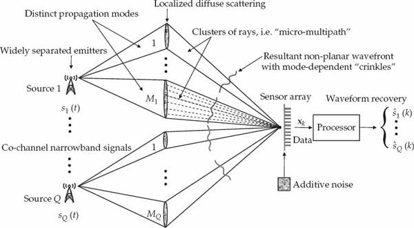
FIGURE 13.1 Conceptual illustration of the blind waveform estimation problem. The illustration depicts a finite impulse response (FIR) multiple-input multiple-output (MIMO) system, which is the most general case considered. The FIR single-input multiple-output (SIMO) system, where there is only one source and multiple echoes is also of interest in a number of practical applications. © Commonwealth of Australia 2011.
It is assumed that the sensor array is connected to a multi-channel digital receiver that samples the incident signal mixture and additive noise in space and time. The objective of the processor is to recover a clean copy of each transmitted source waveform. Ideally, each waveform estimate is as free as possible of contamination from multipath, other signals, and noise.
The first part of this section describes the physical significance of this problem to HF systems that receive signals via skywave propagation, and develops a mathematical model for the space-time samples acquired by the receiver array as inputs to the processor. The data model is described in relatively general terms, and may also be appropriate in other applications not restricted to HF systems or electromagnetic signals. The second part of this section defines the two main tasks of the processor, namely, source waveform recovery and channel parameter estimation. The main assumptions are also summarized for convenience. The final part of this section provides a simple motivating example to show that wavefront distortions caused by diffuse multipath scattering can be exploited to spatially resolve signal modes with closely spaced nominal DOAs.
13.1.1 Multipath Model
Figure 13.2 illustrates the reception of HF signals from distant sources on a ground-based antenna array via reflection from the ionosphere. Multipath arises due to a number of different “layers” or regions in the ionosphere that propagate the HF signal from source to receiver along well-separated (distinct) paths. However, each ionospheric layer does not act as a perfectly smooth specular reflection surface to the incident signal, but rather presents a spatially extended scattering region that transforms the far-field point source into a distributed signal mode at the receiver. The experimental analysis in Part II of this text confirms this characteristic of the ionospheric reflection process for individual HF signal modes.
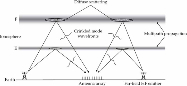
FIGURE 13.2 Notional diagram showing the reception of HF signals via multiple skywave paths. The dominant modes arise from a relatively small number of localized scattering volumes in the E and F regions of the ionosphere. In practice, a layer may have one or more different scattering regions due to the presence of irregularities/disturbances, low- and high-angle modes, as well as magneto-ionic splitting, which produces ordinary and extraordinary waves. This simple diagram illustrates two dominant modes diffusely scattered by the E and F layers, for each source. © Commonwealth of Australia 2011.
Specifically, Figure 13.2 depicts two localized scattering regions at E and F layer heights in the ionosphere. For a particular HF source, each localized scattering region gives rise to an individual signal mode. The physical dimensions of these regions effectively depends on the “roughness” of the isoionic contours that scatter the source signal into the receiver. In practice, there is usually a relatively small number of dominant signal modes that are received from physically separated scattering regions. However, the sum of two or more propagation modes with comparable strength, but different time delays, Doppler shifts, and angles of arrival, can lead to significant frequency-selective fading of the signal received by the system.
The cone of diffusely scattered rays that emanate toward the receiver from each localized scattering region may combine coherently or incoherently with each other. The former case gives rise to a signal mode with a time-invariant crinkled wavefront that carries an amplitude-scaled, time-delayed, and possibly Doppler-shifted copy of the source waveform. In this case, the aim of signal processing at the receiver is to isolate a single ionospheric mode per source, as this recovers a suitable waveform estimate. For example, a spatial filter may be applied to preserve a selected mode from a certain source, while using spare degrees of freedom to null or attenuate other signals received by the array.
In a dynamic propagation medium, the magnitude and phase relationship between the rays diffusely scattered from a localized region will change over time. When the time scale of such changes is long compared to the observation interval, the signal mode impinges on the array as a crinkled wavefront that exhibits an effectively “frozen” spatial structure (approaching the coherently distributed case). However, if the time scale of such changes is short compared to the observation interval, the result is an incoherently distributed signal mode that is characterized by a time-varying crinkled wavefront.
The data model assumed for a multipath signal received by a sensor array will be described in four steps. The first derives a relatively general expression for the analytic continuous-time signal received from a single source. The second incorporates coherently distributed (CD) and incoherently distributed (ID) ray descriptions into this expression to derive a CD and ID signal model. The third converts the continuous-time model to a discrete-time model, which represents the digital samples input to the signal processor. The fourth generalizes this data model to the case of multiple sources. Although the end result is a signal-processing model that can be expressed in a relatively familiar mathematical form, several important steps in the derivation are included to highlight the underlying assumptions required for such a model to be valid in practice.
13.1.1.1 Received Signal
Let the scalar signal g(t) in Eqn. (13.1) be the analytic representation of the narrowband waveform emitted by a source of interest. Here, fc is the carrier frequency, and s(t) is a baseband complex envelope with effective bandwidth B. The narrowband assumption implies a small fractional bandwidth B/fc  1. An alternative definition of narrowband relevant to the development of the model is specified later. Attention is restricted to the single-source case first; the extension to multiple sources is considered later.
(13.1)
Define hn(t, τ) as the time-varying FIR function of the channel that links the source to receiving element n = 1, …, N of the sensor array at time t ∈ [0, To), where To is the observation interval. Note that the variable t denotes continuous time, while τ is the delay variable of the impulse response. For example, the impulse response at time t0 is hn(t0, τ) for τ ∈ [0, Tn), where Tn is the impulse response duration of channel n. The vector h(t, τ) ∈ CN in Eqn. (13.2) represents the multi-channel FIR system function with support over the delay interval τ ∈ [0, Tc), where  is the maximum impulse response duration over all N channels.
(13.2)
The set of complex scalar signals  received by the N elements of the sensor array may be assembled into a spatial snapshot vector x(t) = [x1(t), …, xN(t)]T. In Eqn. (13.3), this vector is defined as the convolution of the source signal with the multi-channel impulse response function, plus measurement noise n(t) ∈ CN. The blind waveform estimation problem assumes that the observations x(t) are accessible, but the system function h(t, τ), source waveform g(t), and additive noise n(t) are not.

(13.3)
Figure 13.3 illustrates the nominal propagation path and cone of diffusely scattered rays for a single dominant mode referred to by the index m. The meaning of narrowband needs to be more carefully defined in two respects. First, it is assumed that the maximum separation between sensors in the array Da is such that the time-bandwidth product condition in Eqn. (13.5) is satisfied, where c is the speed of light in free space. In other words, the elements of the sensor array present a coherent aperture to the rays in a signal mode. Each of these rays is incident as a plane-wave component.
(13.4)
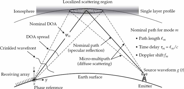
FIGURE 13.3 Schematic diagram showing the nominal path and cone of diffusely scattered rays for a single dominant propagation mode. The time delay, Doppler shift, and DOA of the nominal mode propagation path are indicated. A Doppler shift may arise due to the regular component of large-scale motion of the scattering region, and/or the movement of the source. © Commonwealth of Australia 2011.
Second, it is assumed that diffuse scattering for all dominant modes m = 1, …, M occurs within a localized region such that the maximum time-dispersion of the rays Δm relative to the nominal time delay τm of the mode propagation path is much less than the reciprocal of the signal bandwidth B. In other words, it is assumed that the condition in Eqn. (13.5) is also satisfied.
(13.5)
Provided these conditions are met, h(t, τ) may be written in the form of Eqn. (13.6), where δ(·) is the Dirac delta function. Here, the impulse response is described as the sum of M dominant signal modes with distinct nominal time delays  , where M is assumed to be less than N. Each mode is transferred from source to receiver by its own time-varying channel vector cm(t). This vector represents the instantaneous summation of a large number of rays diffusely scattered from a localized region. In other words, cm(t) represents the time-varying crinkled wavefront of mode m.

(13.6)
Substituting Eqn. (13.6) into Eqn. (13.3) yields the received signal model of Eqn. (13.7). In this model, within-mode ray interference gives rise to relatively “slow” flat-fading. The flat-fading process is embodied in the time-variation of the channel vector cm(t). On the other hand, the summation of M modes with time-delay differences that may significantly exceed 1/B produces relatively “fast” frequency-selective fading. The latter has the potential to significantly distort the temporal signature of the source waveform. Hence, the main objective is to remove frequency-selective fading by isolating one of the dominant signal modes for waveform estimation at the processor output.

(13.7)
For an infinite number (i.e., a continuum) of diffusely scattered rays, the channel vector may be expressed in the form of Eqn. (13.8). The complex scalar function fm(ψ, t) is the time-varying angular spectrum of mode m, where the DOA parameter vector ψ = [θ, φ] includes azimuth θ and elevation φ. The vector v(ψ) ∈ CN denotes the plane-wave array steering vector. This vector represents the spatial response of the sensor array to a single ray that emanates from a far-field point and is incident as a plane wave with DOA ψ.
(13.8)
In the presence of near-field scattering effects and/or array calibration errors, fm(ψ, t) may be interpreted as an equivalent angular spectrum which gives rise to the received channel vector cm(t). However, in this case, fm(ψ, t) loses its physical meaning as the angular spectrum of the scattered rays. Stated another way, this function would then no longer represent the received complex amplitudes of the downcoming rays that impinge on the sensor array from different DOAs.
13.1.1.2 Localized Scattering
A coherently distributed (CD) signal arises due to a scattering process that is effectively “frozen” or deterministic over the observation interval, such that fm(ψ, t) → fm(ψ) for t ∈ [0, To). A limitation of this description is that it does not capture Doppler frequency shifts, which are often significant in practice. Different mode Doppler shifts  may be incorporated into the CD model by assuming the temporal variation of the ray angular spectrum is separable and can be modeled as in Eqn. (13.9).
(13.9)
The presence of a Doppler shift captures the regular component of large-scale movement of the scattering region and source over the observation interval by introducing a linear phase-path variation common to all rays. From Eqn. (13.8), the channel vector cm(t) may then be expressed in terms of a time-invariant mode wavefront am, and nominal mode Doppler shift fm in Eqn. (13.10). The vector am may be interpreted as a crinkled wavefront that does not lie on the plane-wave array manifold in general.

(13.10)
The mode wavefront may alternatively be written as am = αmvm, where αm is a complex amplitude, and vm ∈ CN is a spatial signature vector with fixed L2-norm  = N. The spatial signature may in turn be expressed as the Hadamard (element-wise) product in Eqn. (13.11), where dm ∈ CN is a multiplicative distortion vector that modulates an underlying plane wavefront v(ψm) parameterized by the nominal DOA ψm = [θm, φm] of mode m.
(13.11)
Substituting Eqn. (13.10) and Eqn. (13.11) into Eqn. (13.7) yields the CD diffuse multipath model in Eqn. (13.12), which has been extended to include mode Doppler shifts. The assumption of linearly independent mode wavefronts  is often justified for M < N dominant modes due to the different diffuse scattering processes involved, as well as the differences in the nominal mode DOAs.

(13.12)
The incoherently distributed (ID) signal model gives rise to channel vector variations that are not separable in space and time. After the nominal mode Doppler shift is factored out, this leaves a time-varying mode wavefront, denoted by am(t). If the channel is assumed Gaussian and wide-sense stationary over the observation interval, for example, the mode wavefronts may be statistically described by a mean vector am and covariance matrix Rm, as in Eqn. (13.13). Recall that ∼ CN denotes the complex normal distribution.
(13.13)
Although Rm may have full rank N, most of the energy in the wavefront fluctuations is typically contained in a small number of Im < N eigenvalues. Defining the effective subspace as  , where the columns of Qm are the Im dominant eigenvectors of Rm, the dynamic component of the mode wavefront is well-approximated by Qmςm(t), where
  is a time-varying coordinate vector. In this case, the channel vector takes the form in Eqn. (13.14).
(13.14)
This description incorporates purely statistical ID signals with zero-mean (i.e., am = 0), and partially correlated distributed (PCD) signals, where ςm(t) changes smoothly over time as correlated (dependent) realizations. In the following, there is no requirement to invoke a specific model for am and Qm, such as the Gaussian model alluded to previously. The main assumption is that am is linearly independent of the columns of Qm. As stated earlier, linear independence is also required amongst the different modes. The ID signal model of x(t) is given by Eqn. (13.15).

(13.15)
In this chapter, particular emphasis is on waveform estimation using the CD model that was extended to include Doppler shifts in Eqn. (13.12). The additive noise n(t) may be of ambient or thermal origin, and is notionally considered to be spatially and temporally white. However, arguments are made later to justify the robustness of the developed approach for signals described by the ID model of Eqn. (13.15), and additive noise that is structured or “colored.”
13.1.1.3 Acquired Data
After down-conversion and baseband filtering of the received signal, the in-phase and quadrature (I/Q) outputs are uniformly sampled at time instants  . From Eqn. (13.1), it is straightforward to show that the samples of the source waveform are given by Eqn. (13.16). By ignoring the immaterial phase term
  , we may replace the continuous time signal g(t) by the sampled baseband sequence s(kTs). For the single-source case, the contracted notation sk = s(kTs) will be used.
(13.16)
Based on the CD model in Eqn. (13.12), the array snapshots xk are given by Eqn. (13.17), where νm = fm/fs is the Doppler shift normalized by the sampling frequency (fs = 1/Ts),  m = τm/Ts is the time delay normalized by the sampling period,
  is the received mode wavefront, and nk is additive noise. Provided the time-bandwidth product BTs is smaller than unity (i.e., the signal is not under-sampled), τm is not required to coincide exactly with a time delay bin such that m is an integer). This case is adopted only to simplify the description of the model.

(13.17)
The spatial snapshots xk may be described by the familiar array signal processing model in Eqn. (13.18), where the columns of the multipath mixing matrix contain the M mode wavefronts A = [a1, …, aM], and the M-variate multipath signal vector  contains the source waveform propagated by the different modes. Note that the definition of this vector incorporates the nominal mode time delays and Doppler shifts.
(13.18)
The overall data set consisting of K array snapshots acquired over a processing interval of To seconds may be represented using the matrix notation in Eqn. (13.19), where the N × K data matrix is X = [x1, …, xK], the M × K signal matrix is S = [s1, …, sK], and N = [n1, …, nK] is the noise matrix.
(13.19)
By defining h(k, ) ∈ CN as the discrete-time multi-channel impulse response function, and  as the FIR model order determined by the maximum duration of the channel
  , the array snapshots may be represented in the alternative form of Eqn. (13.20).

(13.20)
It is readily shown that h(k, ) = [h1(k, ), …, hN(k, )]T is given by Eqn. (13.21), where by analogy with the time-continuous FIR channel function hn(t, τ), the complex scalar hn(k, ) denotes the impulse response that links the source to receiving element n at time k with relative delay . This model is representative of an FIR-SIMO system with time-varying channel coefficients.

(13.21)
For a total number of samples K, a time-invariant FIR-SIMO model arises only for an observation interval To = KTs that is sufficiently short to negate the effect of mode Doppler shifts. In other words, the condition νmK 1 is required for all modes m, such that h(k, ) → h(). In this case, the time-invariant multi-channel FIR function is given by Eqn. (13.22).

(13.22)
Use of the CD model extended by Doppler shifts in Eqn. (13.18) suffices for describing the key elements of the waveform estimation problem in the following parts of this section. This model has been presented in the alternative mathematical forms of Eqns. (13.20) and (13.20) to explain its relationship to blind system identification (BSI) and blind signal separation (BSS) techniques described in Section 13.2. The ID version of this model will be considered in Section 13.3, where the GEMS algorithm is described.
13.1.1.4 Multiple Sources
In the case of Q independent sources, the FIR-MIMO system data model of Eqn. (13.23) is a straightforward generalization of the FIR-SIMO model presented in Eqn. (13.3). The Q co-channel sources are assumed to emit different narrowband waveforms gq(t) for q = 1, …, Q. The multi-sensor channel impulse response function for source q is  with maximum time duration Tq. The sources are assumed to be widely separated, such that the FIR channels hqn(t, τ) for all sources q and receivers n are sufficiently diverse to be identifiable. More will be said on the topic of identifiability in Section 13.2.

(13.23)
The same steps taken previously for the single-source case lead us to the discrete-time model of the received array data xk ∈ CN in Eqn. (13.24). The scalar waveform sq(k) to be recovered is the baseband-sampled version of gq(t), where the sample index k is left inside the brackets for the multiple-source case to avoid confusing notation. The number of dominant modes propagated along distinct paths for source q is denoted by Mq. The terms mq, νmq, and amq are the mode time delays, Doppler shifts, and crinkled wavefronts, respectively. The additive noise nk is assumed to be uncorrelated with all sources.

(13.24)
In the adopted FIR-MIMO model, the total number of signal components is  . It is further assumed that multipath is present for all sources, i.e., Mq > 1. With reference to Eqn. (13.18), the array snapshots xk resulting for Q sources may be expressed as in Eqn. (13.25). Here,
  and
and  are the multipath mixing matrix and multipath signal vector for source q, respectively, defined analogously to the single-source case.

(13.25)
The data may be expressed as in Eqn. (13.26), where the N × R matrix H = [A1, …, AQ] contains the wavefronts of all R signal components, while the augmented (source and multipath) signal vector pk ∈ CR is a stacked vector of {s1(k), …, sQ(k)}. Recall that the multipath signal vector sq(k) incorporates the time delays {mq} and Doppler shifts {νmq} for all modes m = 1, …, Mq of source q.
(13.26)
In this case, the totality of the data acquired during the processing interval may be represented in the matrix form of Eqn. (13.27), where the R × K augmented signal matrix P = [p1, …, pK]. This multiple-source model will not be considered in the following parts of this section, but will be used in Sections 13.2 and 13.3.
(13.27)
In anticipation of the discussion in Section 13.2, the FIR-MIMO model is also presented here in an alternative mathematical form. By defining hq(k, ) ∈ CN as the discrete-time multi-channel impulse response function for source q, and  as the associated FIR model determined by
  , the array snapshots may be represented by the convolutive mixture model in Eqn. (13.28).

(13.28)
It is readily shown that hq(k, ) = [hq1(k, ), …, hqN(k, )]T is given by Eqn. (13.29), where by analogy with the time-continuous FIR channel function hqn(t, τ), the complex scalar hqn(k, ) denotes the impulse response component that links source q to receiver n at time k with relative delay . This constitutes an FIR-MIMO system with time-varying channel coefficients.

(13.29)
The time-invariant FIR-MIMO model arises for observation intervals that are sufficiently short to negate the effect of the largest signal Doppler shift over all sources and modes. In other words, the condition Kνmq 1 needs to be met for all (m, q), such that hq(k, ) → hq() given by Eqn. (13.30).

(13.30)
13.1.2 Processing Objectives
In the blind signal-processing problem considered, the objective of the processor is to estimate the source input sequences and propagation channel parameters from noisy measurements of the received signals. In general, the sensor array receives signals from a number of different sources where there are multiple propagation paths per source. To maintain simplicity in the first instance, the processing objectives are described for the case of a single source and multiple echoes (modes) in this section. The more general case involving multiple sources will be dealt with in subsequent sections of this chapter.
Depending on the type of system in question, the primary objective of the processor is often either to estimate the source waveform or channel parameters, depending which of these unknowns is of more interest. However, once either has been estimated through the use of blind signal processing, it is usually straightforward to estimate the other in a subsequent (non-blind) processing step. The signal and channel estimation problems addressed in this chapter are described below. Several practical applications of blind signal and channel estimation not limited to radar are also described. Finally, the main assumptions related to the data model and processing task are summarized to complete the problem formulation.
13.1.2.1 Waveform Estimation
The waveform estimation task is to obtain a clean copy of the signal emitted from the source of interest, where this may be an amplitude-scaled, time-delayed, and possibly Doppler-shifted version of the transmitted baseband modulation envelope. Recovering the source waveform may be regarded as a complementary problem to those of signal detection and source localization. From an array processing perspective, the main aim of spatial filtering is to pass the dominant propagation mode for waveform estimation, and to reject all other interfering multipath signals based on differences in received wavefront structure. According to the signal model of Eqn. (13.18), waveform estimation is tantamount to a multipath separation problem for the single-source case.
Knowledge of the source waveform may be useful for several different reasons depending on the relationship between the signal of interest and system function. Examples of practical systems that can benefit from high-fidelity waveform estimation are mentioned below. Although the significance of the signal to the system is quite different in each case, a common thread is the underlying requirement for an accurate estimate of the source waveform. Fundamental techniques to address this problem therefore have a variety of practical applications, not limited to those described here.
• In communication systems, the primary interest is to extract the information that is encoded in the modulation of the transmitted signal. Minimizing frequency-selective fading caused by multipath at the receiver can reduce signal envelope distortions and significantly improve link performance.
• In passive radar systems, the source waveform is used as a reference signal for matched filtering. The data carried by a signal of opportunity is not of direct interest here, but a clean copy of the source waveform is required to effectively detect and localize echoes from man-made targets.
• In active radar systems, a co-channel source may represent an unwanted signal that can potentially mask useful signals. Knowledge of the source waveform can facilitate the mitigation of such interference, particularly when it is received through the main lobe of the antenna beam pattern.
The clairvoyant1 signal-copy weight vector wm ∈ CN that perfectly isolates mode m from all other modes at the spatial processor output is given by the well-known minimum-norm solution in Eqn. (13.31). Recall that A is the multipath mixing matrix defined previously. The vector um ∈ CM has unity in position m and zeros elsewhere, while β is an arbitrary complex scalar that does not affect output signal-to-noise ratio (SNR). The symbol † denotes the Hermitian (conjugate-transpose) operator.
(13.31)
From the model in Eqn. (13.18), the clairvoyant signal-copy weights wm yield the output zk in Eqn. (13.32), where  is the desired estimate of the source waveform, and
  is a residual noise contribution. This deterministic “null-steering” spatial filter estimates a copy of the source signal that is free of multipath contamination. Among all the linear combiners that produce a multipath-free estimate, wm maximizes the output SNR in the case of spatially white additive noise.
(13.32)
The optimum filter maximizing the output signal-to-interference-plus-noise ratio (SINR) is given by Eqn. (13.33), where Qm is the statistically expected spatial covariance matrix of all the unwanted signal modes plus noise. The optimum filter is in general different to wm, but tends to the expression in Eqn. (13.31) when the interfering modes are not coherent and much more powerful than the additive noise.
(13.33)
In the spatial processing context, the objective of blind source waveform recovery is to estimate the weights wm for a multipath-free output, or  for an output with minimum mean-square error, depending on which criterion is deemed most desirable. Application of the weight vector to the received array snapshots yields an amplitude-scaled, time-delayed, and possibly Doppler-shifted estimate of the source waveform at the spatial filter output, which fulfils the processing objective.
The key point is that the mixing matrix A = [a1, …, aM] is unknown a priori, and supervised training to estimate Qm is not possible in the considered problem. The model order M and wavefronts am can be estimated under certain conditions, as described in Section 13.2. However, errors in the reconstruction of A due to estimation uncertainty or model-mismatch will lead to the output being corrupted by residuals of the interfering modes, which can significantly reduce the SINR, and hence quality of the waveform estimate.
13.1.2.2 Channel Estimation
The channel impulse response or system function is of more direct interest in certain applications than the source input sequence. In the model of Eqn. (13.20), the channel parameters are the number of modes M, the nominal delay, and Doppler shift of each mode {τm, fm}, and the mode wavefronts  from which the nominal mode DOAs ψm may be inferred.
In practice, it is not always possible to determine the absolute (as opposed to relative) values of certain channel parameters. This is due to the ambiguity in attributing absolute values uniquely to the channel or source. In addition to the obvious ambiguity in complex scale αm, the absolute time delays τm and Doppler shifts fm of the channel are unobservable from xk without further information about the source. Hence, the objective of channel parameter estimation is to estimate M and the relative mode complex-scales, time-delays, and Doppler-shifts, in addition to the wavefront structure and nominal DOA of each mode.
Knowledge of the propagation channel parameters can have a number of practical uses. In communication systems, traditional methods for multipath channel equalization require the transmission of training symbols or pilot sequences prior to the data frame. This enables the channel parameters to be estimated so that compensation for multipath can be applied to the information-carrying signals. However, training signals may be not be available in some cases, for instance when the source is uncooperative or occurs due to natural phenomena. This has motivated the development of blind system identification techniques that aim to estimate the channel parameters without a requirement for training sequences. Such techniques will be discussed in Section 13.2.
In the HF band, information about the nominal mode DOAs ψm and relative time delays τm may be used in conjunction with an ionospheric model to estimate the position of an uncooperative source. Geolocation of unknown HF sources from a single site is a problem of interest to the HF direction-finding community. The inverse problem of using uncooperative HF sources at known locations as reference points to estimate ionospheric reflection heights, and possibly tilts, is of significant interest for coordinate registration in OTH radar. Although the emphasis in this chapter is to address the blind source waveform recovery problem, blind estimation of the propagation channel parameters will be illustrated for an HF single-site location (SSL) application in Section 13.6.
13.1.2.3 Main Assumptions
The main assumptions related to the model of Eqn. (13.18) are summarized here to complete the problem formulation. With reference to Eqn. (13.18), these assumptions pertain to the source waveform sk, the mixing matrix A, the nominal mode delays τm, and Doppler shifts fm. The generalization of these assumptions for the multiple-source case will be described in Section 13.3.
1. Source Complexity: The narrowband assumption described earlier is a necessary but not sufficient condition as far as the source waveform is concerned. In order to ensure the blind signal estimation problem is identifiable, the source waveform is required to have a finite bandwidth, such that sk is not a constant or sinusoid, for example. Specifically, the input sequence is required to have a linear complexity P > 2L, where L is the maximum FIR model order over all N channels. Linear complexity of a finite-length deterministic sequence  is defined as the smallest integer P for which there exist coefficients
  that satisfy Eqn. (13.34) for all k = 1, …, K.

(13.34)
As virtually all finite bandwidth signals of interest satisfy this linear complexity condition for realistic HF channels, the source waveform may be considered to have a practically arbitrary temporal signature. Importantly, no further information is assumed regarding the deterministic structure or statistical properties of the source waveform, which is therefore not restricted to having any particular modulation format. Clearly, the source is assumed to be uncooperative in the sense that training symbols or pilot signals are not available for estimation purposes.
2. Channel Diversity: The source waveform is assumed to be received as an unknown number M of diffusely scattered dominant modes, where 1 < M < N. In other words, multipath propagation is assumed to exist, but the number of dominant modes is less than the number of receiving elements. In addition, the mode wavefront vectors am ∈ CN for m = 1, …, M are assumed to form a linearly independent set, such that the multipath mixing matrix has full rank. These requirements are expressed in Eqn. (13.35), where the operator R{·} returns the rank of a matrix.
(13.35)
Apart from satisfying these conditions, which ensure the system is identifiable and that the problem is not ill-posed, no other information is assumed about the mixing matrix. This implies that {a1, …, aM} are otherwise arbitrary vectors, which are not confined to lie on or close to a parametrically defined spatial signature manifold, such as the plane-wave steering vector model. It follows that the sensor array is not restricted to a particular geometry, and that array manifold uncertainties due to nonidentical element gain and phase responses, sensor position errors, and mutual coupling can be tolerated.
3. Sample Support: This assumption relates to the acquisition of sufficient data in the processing interval, such that enough samples exist to determine the number of system unknowns. From Abed-Meraim, Qui, and Hua (1997), the number of samples K required to ensure identifiability needs to satisfy the condition in Eqn. (13.36), where L is the maximum channel impulse response duration defined previously. More will be said on the subject of identifiability in Section 13.2.
(13.36)
4. Distinct Modes: Besides the quite mild conditions assumed for A, sk, and K above, the number of modes M and the associated delay-Doppler parameters  are also assumed to be unknown. The differences between the mode parameter tuples ρm = [m, νm] are assumed to be distinct, as in Eqn. (13.37). Note that this condition applies to the relatively small number of dominant signal modes and not the diffusely scattered rays within each mode.
(13.37)
Except for certain contrived scenarios, the differential delay and Doppler between two distinct modes (i ≠ j) will in general not be identical to that of another pair of modes (n ≠ m) when attention is restricted to the few dominant modes.
13.1.3 Motivating Example
Diffusely scattered signals are present in a variety of fields. In wireless communications, they are produced by “local scattering” in the vicinity of mobile transmitters, particularly where there is no line-of-sight between the transmitter and receiving base-station, see Zetterberg and Ottersten (1995); Pedersen, Mogensen, Fleury, Frederiksen, Olesen, and Larsen (1997); Adachi, Feeney, Williamson, and Parsons (1986); and Ertel, Cardieri, Sowerby, Rappaport, and Reed (1998) for example.
In sonar, large hydrophone arrays are used to localize spatially distributed acoustic sources that have distorted wavefronts due to propagation in the heterogeneous underwater channel (Owsley 1985). Distributed signals with non-stationary wavefront amplitude and phase “abberations” are also observed in ultrasonics due to irregular propagation through tissue, where wavefronts received over different paths are noticed to experience different distortions; see Liu and Waag (1995, 1998) and Flax and O’Donnell (1988). A similar phenomenon is encountered in radio astronomy due to “scintillation” of signals as they pass through nonuniform plasma profiles (Yen 1985). Blind spatial processing techniques based on distributed multipath signal models may, therefore, find uses in diverse applications.
Before proceeding to a brief review of existing techniques for BSI and BSS, a simple example is used to illustrate how wavefront distortions may assist to separate signal modes with closely spaced nominal DOAs. This is a common problem due to the limited spatial resolution of practical sensor arrays, the fact that multipath components are often received from very similar directions, and that super-resolution techniques for DOA estimation are highly sensitive to model mismatch. A notorious example in microwave radar is the low-elevation multipath encountered over seawater between an airborne source and the receiving antenna array on a surface vessel.
The motivating example described below is relevant to HF radar and directly related to a real-world scenario where data has been collected and processed in Section 13.4. Suppose there are M = 2 signal modes, and the goal is to pass mode m = 1 and perfectly cancel mode m = 2. The clairvoyant minimum-norm signal-copy weight vector that accomplishes this task is given by w1 = βA(A†A)−1u1, where A = [v1, v2] may be defined in terms of the spatial signatures vm instead of the mode wavefronts am without loss of generality.
The SNR gain in white noise, defined as the SNR of mode 1 at the linear combiner output SNRo relative to that in the reference (first) receiver of the array SNRi, is given by SNRg = SNRo/SNRi = |β|2/|| w1||2. The L2-norm || w1||2 may be evaluated by substituting A = [v1, v2] and u1 = [1, 0]T into Eqn. (13.38), and noting that the determinant of (A†A) is given by ∇ = ad − bc, where a = || v1||2,  ,
,  , and d = || v2||2.
(13.38)
From Eqn. (13.38), SNRg = ∇/|| v2||2, and after evaluating the determinant  , it is straightforward to show that SNRg is given by Eqn. (13.39). The maximum SNR gain with which mode 1 can be estimated with no contamination from mode 2 in white noise depends on the magnitude-squared coherence (MSC) between the spatial signatures:
  , where ϒ is the angle between v1 and v2 in N-dimensional space. The highest SNR gain subject to the constraint of no multipath interference at the output is || v1||2. This is precisely the matched filter gain, attainable only when the spatial signatures are orthogonal
  , such that cos2 ϒ = 0. For all other cases, the SNR gain is smaller and tends to zero as the spatial signatures align, i.e., as cos2 ϒ → 1.

(13.39)
The improvement in SNR gain due to the presence of “crinkled wavefronts,” relative to the hypothetical case of specular reflection which gives rise to plane waves with the same DOAs (nominal DOAs for diffuse scattering), is denoted by SNRIF in Eqn. (13.40). This is simply the ratio of SNR gains in Eqn. (13.39) occurring for the two cases. Here, cos2 Φ = F{v(ψ1), v(ψ2)} is the MSC for plane waves at the nominal mode DOAs, and cos2 ϒ is the MSC for the mode spatial signatures  with multiplicative distortions {dm}m=1,2. When the nominal mode DOAs are closely spaced (ψ1 → ψ2), we have that cos2 Φ → 1 and hence the denominator Δ = (1 − cos2 Φ) → 0. As ψ1 → ψ2, cos2 ϒ → cos2 Θ, where cos2 Θ = F{d1, d2} is the MSC of the multiplicative distortion vectors. Hence, SNRIF → sin2 Θ/Δ, where Δ → 0, as ψ1 → ψ2. Large improvements in output SNR can result provided that the distortions {dm}m=1,2 are sufficiently different, so that sin2 Θ
  Δ.
Δ.

(13.40)
Thus, when the mode nominal DOAs are closely spaced, different distortions caused by independent diffuse scattering processes can be exploited to estimate the waveform with no multipath contamination at higher output SNR.2 This situation is particularly relevant for an HF source located close to boresight of a linear array, where ionospheric modes reflected from different layers share similar nominal cone angles, but are likely to exhibit different wavefront distortions due to the independent diffuse scattering processes.
This illustrative example motivates the use of manifold-free procedures that can take advantage of wavefront distortions for separating signal modes with closely spaced nominal DOAs. Moreover, reliance on the plane-wave model when distortions are actually present would lead to higher SINR improvements than those predicted by Eqn. (13.40).
13.2 Standard Techniques
Standard techniques relevant to the formulated problem fall under two main classes, namely, multi-channel blind system identification (BSI), and blind signal separation (BSS). The former typically assumes the presence of a single source and models the propagation channel linking the source to each receiving element of the array by a different finite impulse response (FIR) function. In the standard multi-channel BSI problem, the source input sequence and FIR system function are both assumed to be unknown. At times, the main intent is to estimate the system function, as opposed to the input sequence, which may be viewed merely as a probing signal. However, the problem can be easily recast to estimate the input sequence directly. In any case, multi-channel BSI techniques often involve the joint processing of a block of space-time data to estimate the unknown parameters.
As its acronym suggests, BSS techniques assume the presence of multiple sources, where the emitted signals cannot be separated by simple operations, such as bandpass filtering. In the array processing context, many BSS techniques assume an instantaneous mixture model, wherein the signals propagate directly from source to receiver without multipath reflections. This is called an instantaneous multiple-input multiple-output (I-MIMO) system. Such a system is appropriate for applications that involve line-of-sight propagation, for example. Alternative BSS techniques address the problem of convolutive signal mixtures, where the presence of multipath gives rise to an FIR-MIMO system. In any case, the aim of multi-channel BSS techniques is to separate and estimate the different source signals from the received array data. This is commonly achieved by spatial-only processing, although space-time processing may be used.
The first purpose of this section is to provide background and reference material on the subjects of multi-channel BSI and BSS. This includes a description of the data models often adopted in standard BSI and BSS approaches, with both the I-MIMO and FIR-MIMO systems considered in the latter case. The second purpose is to provide an overview of the underlying assumptions upon which many existing BSI and BSS techniques are based. This is undertaken with a view to determining whether such techniques are applicable to the previously formulated problem. A discussion at the end of this section motivates the development of a new blind waveform estimation technique, referred to as Generalized Estimation of Multipath Signals (GEMS).
13.2.1 Blind System Identification
Traditional approaches for multipath equalization require the scheduling of training data sequences on transmit, which can significantly consume channel capacity and system resources in a time-varying environment (Paulraj and Papadias 1997). Moreover, training data is obviously unavailable when the signal of interest is transmitted by an uncooperative source. These factors have led to the development of BSI techniques, also known as blind channel equalization or blind deconvolution. A detailed description of BSI techniques is beyond the scope of this text, but comprehensive treatments can be found in the excellent review articles of Abed-Meraim et al. (1997), Tong and Perreau (1998), as well as the text of Haykin (1994), for example.
Figure 13.4 shows a discrete-time representation of the standard multi-channel BSI problem. The source produces a scalar input sequence sk, which is received at sensors n = 1, …, N after propagation through a linear channel with an impulse response function hn(). Multi-channel BSI is traditionally based on a time-invariant FIR model of each channel hn() with support over a delay interval = 0, …, L. Recall that L is defined as the maximum FIR model order for the N-channel system. According to this model, the complex data sample xnk received by sensor n at time k is given by Eqn. (13.41), where nnk is additive noise independent of the signal.
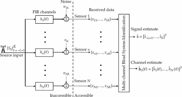
FIGURE 13.4 Representation of the standard multi-channel BSI architecture as a time-invariant FIR-SIMO system. The FIR model order is L, the number of sensors is N, and the number of data samples received by each sensor is K. The source input sequence, channel impulse responses, and additive noise processes are assumed to be inaccessible. The objective of the BSI processor is to jointly identify the source signal and channel coefficients from the observed space-time data to within a complex scale ambiguity. © Commonwealth of Australia 2011.

(13.41)
The source input sequence sk and multi-channel system function h() = [h1(), …, hN()]T are assumed to be inaccessible. Only the time-series data yn = [xn1, …, xnK]T received by the N-sensor array is deemed to be observable. The vector yn ∈ CK may be expressed in the form of Eqn. (13.42).
(13.42)
In Eqn. (13.42), Hn ∈ CK×(K+L) is the Sylvester matrix containing the impulse response of channel n, as defined in Eqn. (13.43). For K output samples in yn, it follows that s = [s−L+1, …, sK]T is the (K + L)-dimensional vector of input samples extended by the maximum FIR model order L, and ∈n = [nn1, …, nnK]T is the K-dimensional vector of additive noise.

(13.43)
Alternatively, the data vector yn may be written in the form of Eqn. (13.44), where S ∈ CK×(L+1) is the Toeplitz matrix of the input sequence extended by the maximum FIR model order L, and hn = [hn(0), …, hn(L)]T is the (L + 1)-dimensional vector of the impulse response coefficients of channel n.
(13.44)
To be clear, S ∈ CK×(L+1) is defined in Eqn. (13.45). This representation is relevant to supervised channel estimation using a known input sequence. In this case, S is known during the training interval, and R{S} = L + 1 by design. The channel coefficients may be estimated from the received data as  n = S+yn = hn + S+∈n, where S+ = (S†S)−1S†.

(13.45)
The total data acquired by the time-invariant FIR-SIMO system over the processing interval may be written as Eqn. (13.46), where  is the NK-dimensional stacked vector of space-time samples, H ∈ CNK×(K+L) is the generalized Sylvester matrix formed by stacking {H1, …, HN}, and ε ∈ CNK is the stacked vector of additive noise, constructed similar to y.
(13.46)
Using Eqn. (13.44), it is also possible to write y in the form of Eqn. (13.47), where  is the stacked vector of the N channel impulse response functions, and the NK × N(L + 1) matrix SN = diag{S, …, S} is formed as N diagonal blocks each containing the Toeplitz matrix of the input sequence S defined in Eqn. (13.45).
(13.47)
When training data is available to estimate the channel coefficients as  , linear space-time equalization may be applied to estimate the input sequence from the received data as in Eqn. (13.48). This assumes NK > (K + L) and that H has full column-rank (K + L). However, when the channel and source are both unknown, the variables H and s need to be estimated jointly from the observations y (i.e., blindly).
(13.48)
For additive white Gaussian noise, application of the maximum-likelihood (ML) criterion for the joint estimation of the system matrix H and input sequence s, when neither is known, requires finding the solution to Eqn. (13.49), which is a nonlinear optimization problem. An elegant two-step ML method for calculating (,  )ML is given in Hua (1996). If the FIR-SIMO system is time-varying, because of Doppler shifts for example, frequent updates of this procedure are needed to counter channel variations.
(13.49)
An attractive feature of the BSI approach is that the source input sequence and polynomial channel coefficients can be estimated under relatively general identifiability conditions. The FIR-SIMO system described by Eqn. (13.46) is considered identifiable when a given output y implies a unique solution for the system matrix H and the input sequence s up to an unknown complex scalar in the absence of noise. In accordance with Hua and Wax (1996), the sufficient identifiability conditions for a time-invariant FIR-SIMO system of known model order L are
• The N polynomial sub-channels do not share a common zero. This condition reflects the need for coprime FIR sub-channels (i.e., sufficient channel diversity).
• The input sequence has linear complexity P > 2L. This implies that the input cannot be a constant or sinusoid for example (i.e., sufficient signal complexity).
• The total number of samples K > 3L. This reflects the need for enough data to determine the number of system unknowns (i.e., sufficient sample support).
However, standard BSI approaches also have some known limitations. For example, the FIR model order is often unknown in practice, and its estimation is a challenging problem (Abed-Meraim et al. 1997). BSI performance can be sensitive to poor estimation of L. Moreover, sparse channels that are highly time-dispersive may require large values of L for equalization, despite the possible presence of few dominant propagation modes, i.e., L M. This leads to multi-channel equalizers of large dimension N(L + 1), which increases demands on finite sample support, not to mention computational load.
In addition, large Doppler shifts may stipulate the use of very short data frames to satisfy the time-invariant channel assumption. This restricts the observation interval that can be coherently processed (Hua 1996). The requirement for fast updates may also reduce sample support and increase computational load. These factors can limit the practical performance of standard BSI approaches. This motivates the search for alternative methods that are less prone to these drawbacks, yet strive to retain the general identifiability conditions of the BSI problem formulation.
It is evident from Figure 13.4 that the spatial snapshot data vector xk = [x1k, …, xNk]T is given by Eqn. (13.50), where h() = [h1(), …, hN()]T The standard BSI model may be reconciled with the CD data model in Eqn. (13.20) by substituting  into Eqn. (13.50). This impulse response function model was derived in Eqn. (13.22) for the case of a narrowband source, local scattering, and M dominant modes received by a coherent sensor array, where the length of the data record is sufficiently short to neglect the mode Doppler shifts.

(13.50)
Two comparative remarks are made. First, the multi-channel impulse response function h() is assumed to be time-invariant in the standard BSI model, whereas Doppler shifts give rise to a time-varying impulse response function h(k, ). Importantly, standard BSI approaches are not designed to handle a time-varying impulse response function during the observation interval. Recall that the CD model was extended to include the effect of mode Doppler shifts, which may be significant in the problem considered.
Second, standard BSI approaches are not designed for the case of multiple sources, where it is required to estimate the waveform of each source. On the other hand, the FIR model of h() in the BSI problem is general in the sense that it is also applicable to broadband signals, extended scattering, and receiving arrays with widely spaced sensors. In other words, the FIR structure of h() in Figure 13.4 is not restricted to the form of Eqn. (13.22).
13.2.2 Blind Signal Separation
Multi-channel BSS methods are applied to separate and recover the waveforms of multiple sources received by a sensor array, where the different signals cannot be discriminated readily in time or frequency. In the spatial processing context, the vast majority of BSS techniques, also referred to as “unsupervised” or “self-recovering” methods, fall into two main categories: (1) those which make certain assumptions regarding the propagation channel and sensor array in order to characterize the spatial signatures of the signals to be estimated, i.e., manifold-based methods, and (2) those which are not based on a manifold model but instead utilize a priori information regarding some known deterministic or statistical properties of the waveforms to be separated, i.e., source-based methods. In-depth treatments of manifold- and source-based BSS methods can be found in Van Der Veen (1998) and Cardoso (1998), respectively.
BSS using spatial processing is a topic that has received enormous attention in the literature. Figure 13.5 shows a top-level breakdown of BSS techniques, including source-based methods, manifold-based methods, and the alternative of exploiting multipath as the enabling physical mechanism. A brief overview of the many works existing on manifold-and source-based BSS methods is provided in this section. By comparison, relatively few works in the open literature have directly exploited multipath as the mechanism for enabling blind source separation.
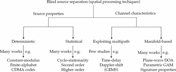
FIGURE 13.5 Taxonomy of standard BSS approaches in terms of underlying assumptions used as the basis for separation. The lack of information about the source signals has in many works been remedied by assuming partial knowledge about the propagation channel and sensor array, such that parametric spatial signature models may be used for separation. On the other hand, alternative approaches assume that certain deterministic or statistical properties are known about the source waveforms in order to compensate for the lack of knowledge regarding the propagation channel and sensor array characteristics. In the spatial processing context, relatively few works have directly exploited multipath as the physical mechanism to enable BSS. The GEMS algorithm is based on the concept that this alternative approach may be used to relax the assumptions required for the source waveforms and array manifold, jointly, rather than separately. © Commonwealth of Australia 2011.
Importantly, it will be shown that this approach allows certain assumptions regarding both the source and manifold to be relaxed. The GEMS algorithm exploits multipath for signal separation under relatively mild assumptions regarding both the mode wavefront and source waveform properties. It is precisely the mildness of these assumptions that makes the GEMS approach noteworthy and robust.
The I-MIMO system is schematically depicted in Figure 13.6, where source q is linked to channel n by a complex scalar transfer coefficient aqn. The received array snapshot xk = [x1k, …, xNk]T can be represented in the standard form of Eqn. (13.51) where the N × Q instantaneous source mixing matrix A = [a1, …, aQ] contains the Q channel vectors, denoted by aq = [aq1, …, aqN]T for q = 1, …, Q, while the Q-dimensional source signal vector s(k) = [s1(k), …, sQ(k)]T contains the different input sequences.
(13.51)
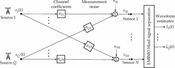
FIGURE 13.6 Illustration of the instantaneous multiple-input multiple-output (I-MIMO) system model. The source input sequences, complex-scalar channel transfer coefficients, and additive noise processes are inaccessible. The objective of the BSS processor is to jointly estimate all of the source waveforms to within an unknown complex scale by spatially weighing and combining the received array data. © Commonwealth of Australia 2011.
The source signal vector s(k) should not be confused with the multipath signal vector sk in Eqn. (13.18). The instantaneous source mixing matrix A also has a different physical interpretation to the multipath mixing matrix A in Eqn. (13.18). However, it is apparent that Eqn. (13.51) has an equivalent mathematical form to Eqn. (13.18) in the special case where the Q sources are assumed to emit signals that are time-delayed and Doppler-shifted versions of a common input sequence, as in Eqn. (13.52). From the BSS viewpoint, there is clearly no distinction between Eqns. (13.18) and (13.18) in this special case.
(13.52)
The FIR-MIMO system model illustrated in Figure 13.7 is of more direct interest for multiple sources propagated over multipath channels. Indeed, the FIR-MIMO framework generalizes the BSI problem in Figure 13.4 to the multiple-source case. In Figure 13.7, hqn() for = 0, …, L denotes the FIR function of the channel that links source q to sensor n. It follows from the single-source expression in Eqn. (13.50) that the FIR-MIMO spatial snapshots xk are given by Eqn. (13.53), where hq() = [hq1(), …, hqN()]T and 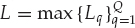 is the maximum FIR model order.

(13.53)
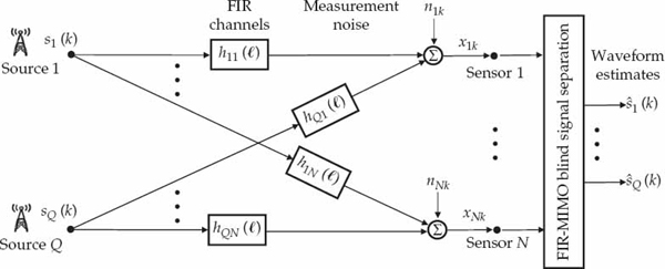
FIGURE 13.7 Illustration of the FIR multiple-input multiple-output (FIR-MIMO) system model. The source input sequences, channel impulse responses, and additive noise processes are inaccessible. The objective of the BSS processor is to jointly estimate all of the source waveforms to within an unknown complex scale by spatially weighting and combining the received array data. © Commonwealth of Australia 2011.
The connection between Eqn. (13.53) and the multiple-source model of Eqn. (13.51) developed in the previous subsection becomes evident if we substitute the time-varying impulse response  for hq() in Eqn. (13.53). Making this substitution yields the received data snapshots in Eqn. (13.54), where
 . This expression is consistent with the model of Eqn. (13.24). Note that the definition of
  incorporates the Doppler shift of each mode in the waveform to be estimated. This effectively accounts for channel variations by modifying the waveform of each mode by a different Doppler shift.

(13.54)
The form of Eqn. (13.54) indicates that BSS techniques based on a time-invariant channel model are in principle applicable to the formulated problem since each mode waveform may be considered as a different signal to be estimated. The critical issue here is whether the assumptions required by standard BSS techniques to recover suitable waveform estimates in such a situtation are compatable with those previously set out in the problem formulation. This point will be considered in Section 13.2.3 with reference to the multiple-source model reproduced in Eqn. (13.55), and the single-source model X = AS + N described in the previous section.
(13.55)
In the single-source case, the identifiability condition relating to channel diversity implies that the mode wavefronts in the mixing matrix A are linearly independent so that A has full column-rank M, while the identifiability condition relating to input sequence linear complexity implies that the signal matrix S has full row-rank M. This leads to the fundamental property upon which nearly all BSS techniques are based, namely, that the column span of X provides a basis for the column span of A, and that the row span of X provides a basis for the row span of S. Similar concepts apply for the multiple-source case.
13.2.2.1 Manifold-Based Methods
A popular manifold-based method is to discriminate the signals on the basis of differences in DOA by assuming a plane-wave model. Such a model is valid for narrowband signals and point sources in the far-field of a well-calibrated sensor array. This approach may be used to resolve a number of independent sources, or multiple propagation modes from a single source, that impinge on the array as plane waves. In the latter case, specular reflection of the multipath components is often assumed.
Super-resolution techniques such as MUSIC (Schmidt 1981), ESPRIT (Roy and Kailath 1989), MODE (Stoica and Sharman 1990b), WSF (Viberg, Ottersten, and Kailath 1991), ML (Stoica and Sharman 1990a), and their variants described in Krim and Viberg (1996), may be used to resolve signals with closely spaced DOAs. These techniques may be considered “blind” in the sense that the source properties and mixing matrix are not known a priori. In this case, lack of knowledge regarding the source properties is compensated for by assuming the spatial signatures in the mixing matrix lie on a manifold with a known parametric form. Specifically, the plane-wave manifold is defined by the DOA parameter alone.
DOA estimates of the incident signals are used to reconstruct the mixing matrix, which allows a deterministic null-steering weight vector to estimate the individual source waveforms with reduced contamination from multipath components and other signal sources. This is the classic “signal-copy” procedure. Ideally, the first step estimates the exact DOAs of all signal components, while the second step adjusts the weights of the linear combiner to perfectly null all interfering signals, leaving only the desired source waveform and measurement noise at the output. This signal-copy procedure is effective provided that the number of plane-wave signals is less than the number of receivers, the signal DOAs are not too closely spaced, the model order is selected appropriately, and the SNR is adequate for the amount of training data available. In this event, performance is limited mainly by statistical errors.
However, the plane-wave assumption is rather strong and seldom holds in practical scenarios. In particular, diffuse scattering caused by an irregular propagation medium, combined with the presence of array calibration errors, may lead to significant deviations between the spatial signatures of the signals received by the system and the presumed plane-wave manifold model. Diffuse scattering has been observed and analyzed in a number of different fields not limited to wireless communications (Zetterberg and Ottersten 1995), radio astronomy (Yen 1985), underwater acoustics (Gershman, Turchin, and Zverev 1995), speech recognition (Juang, Perdue, and Thompson 1995), medical imaging (Flax and O’Donnell 1988), seismology (Wood and Treitel 1975), and radar (Barton 1974).
In the HF band, point-to-point communication systems and OTH radars that rely on skywave propagation experience diffuse scattering from different horizontally stratified regions or layers in the ionosphere (Fabrizio, Gray, Turley 2000a). In such applications, a spatially distributed signal representation is often more appropriate than a point-source model. Super-resolution methods for DOA estimation may be applied, but even small departures from the plane-wave model can seriously degrade unwanted signal rejection, and hence waveform estimation quality. Performance degradations tend to be most pronounced for small array apertures, closely spaced sources, and powerful signal components; see Swindlehurst and Kailath (1992) and Friedlander and Weiss (1994), for example.
For DOA-based signal-copy procedures, the problem of spatially distributed signals amounts to decomposing the received (non-planar) wavefronts as a sum of vectors on the plane-wave manifold (Van Der Veen 1998). Estimating the DOAs of possibly a very large number of diffusely scattered rays for each distributed signal component represents a formidable task. In many cases, this task is infeasible due to the limited number of receivers and resolution available. Consequently, generalized array manifolds (GAM) not confined to the plane-wave model have attracted significant attention for spatial signature estimation as well as the parametric localization of coherently and incoherently distributed sources. For more information on this topic, the reader is referred to the works of Swindlehurst (1998), Jeng, Lin, Xu, and Vogel (1995), Lee, Choi, Song, and Lee (1997), Raich, Goldberg, and Messer (2000), Meng, Stoica, and Wong (1996), Astely, Ottersten, and Swindelhurst (1998), Trump and Ottersten (1996), Valaee and Champagne (1995), Fabrizio, Gray, and Turley (2000), Besson, Vincent, Stoica, and Gershman (2000), Besson and Stoica (2000), Astely, Swindlehurst, and Ottersten (1999), Weiss and Friedlander (1996), and Stoica, Besson, and Gershman (2001).
Although more flexible than the plane-wave manifold, many GAM models are nevertheless based on certain assumptions. For example, the GAM proposed in Astely et al. (1998) is based on a first-order Taylor series expansion that requires the angular spread of the signal to be small for accurate modeling. On the other hand, DOA-independent and amplitude-only wavefront distortions were assumed in Weiss and Friedlander (1996) and Stoica et al. (2001), respectively. In Valaee et al. (1995), angular spectrum profiles that are known analytic functions of a nominal DOA and spatial spread parameter are presumed to be available. Despite broadening the domain of applicability with respect to the plane-wave manifold, such models may not be general enough to accurately capture an arbitrary set of linearly independent spatial signatures.
In many real-world environments, the spatial signatures may have large angular spreads. Moreover, the received wavefronts typically exhibit a combination of gain and phase distortions relative to the plane-wave model that may differ significantly from one signal component to another. Such distortions can be very difficult to accurately characterize due to the complex diffuse scattering processes involved. Although DOA-and GAM-based techniques are applicable to particular classes of problems, where the assumptions made can be physically justified, they may not allow an arbitrary set of linearly independent spatial signatures to be effectively modeled and resolved for waveform estimation purposes. This restriction can limit the performance of manifold-based methods in practical applications.
13.2.2.2 Source-Based Methods
Performance degradations caused by the sensitivity of manifold-based methods to model mismatch between the actual and presumed signal spatial signatures may be avoided by resorting to a different class of BSS techniques, which are based on source properties as opposed to channel and array characteristics. The purported advantage of source-based BSS techniques stems from the fact that many human-made signals have certain properties that are accurately known a priori in a number of applications. This leads to more robust algorithms, which do not depend on reliable array calibration, or well-understood channel characteristics (Van Der Veen 1998).
For example, BSS may be based on the constant-modulus property of frequency modulated or phase-coded signals, as in Treichler and Agee (1983), van der Veen and Paulraj (1996), and Papadias and Paulraj (1997), or on finite-alphabet signals with known constellations, as in Yellin and Porat (1993), Anand, Mathew, and Reddy (1995), and Talwar, Viberg, and Paulraj (1994), for example. BSS may also exploit known properties regarding the signal second-order statistics (SOS), such as cyclostationarity, which is often encountered in digital communications due to the bauded nature of the transmissions; see Agee, Schell, and Gardner (1990), Xu and Kailath (1992), and Wu and Wong (1996), for example. BSS methods based on the joint diagonalization of spatial covariance matrices have been developed to separate uncorrelated signals in Belouchrani, Abed-Meraim, Cardoso, and Moulines (1997), but such techniques may not be appropriate in multipath environments, where the signals to be separated are often correlated.
Deterministic properties, such as parametrically known templates of periodic radar signals, or the known pulse-shape and code-vectors of CDMA signals, may also be utilized for BSS. Examples of the latter include Liu and Xu (1996), and Liu and Zoltowski (1997). For non-Gaussian signals, the joint distributional properties of the source signals, such as mutual independence, may be used to separate signals based on higher order statistics (HOS), as in Cardoso and Souloumiac (1993), Porat and Friedlander (1991), Dogan and Mendel (1994), Gonen and Mendel (1997), and Yuen and Friedlander (1996). However, the slow convergence rate of the higher order moment sample estimates often poses significant limitations for small data volumes. Perhaps more importantly, cumulant-based methods are not applicable to Gaussian signals, which often emerge from a large number of superimposed rays with random amplitudes and uniformly distributed phases.
Many waveforms emitted by natural and human-made sources of potential interest do not belong to a class of signal with known deterministic or statistical properties that can be utilized for BSS. Specific assumptions regarding the modulation format of a signal can be restrictive in some BSS applications. For this reason, there is value in broadening the scope of BSS techniques by allowing the waveforms to have a practically arbitrary temporal signatures, subject to satisfying the condition required for identifiability (Hua and Wax 1996). Apart from satisfying identifiability, no further knowledge may be available regarding the deterministic or statistical properties of the waveforms to be estimated. Within this more general framework, it would appear that none of the above-mentioned source-based methods are designed for such applications due to the additional information they assume about the source waveforms.
13.2.3 Discussion
There is a perceived lack of blind spatial processing techniques in situations where neither of the premises relied upon by manifold- or source-based BSS methods apply. Specifically, manifold-based methods that assume a plane-wave model or GAM characterization of the received wavefronts may not be capable of describing a completely arbitrary set of M linearly independent spatial signatures using a relatively small number of parameters. On the other hand, source-based methods that depend on certain deterministic or statistical properties of the M signals to be separated may not be flexible enough to deal with practically arbitrary waveforms that are only required to satisfy the linear complexity condition needed for identifiability.
The motivation behind GEMS is to exploit multipath propagation to significantly relax assumptions with regard to both the source signals and spatial signatures. In addition, rather than considering diffuse scattering as a nuisance or complicating factor in the BSS problem, the contrary idea is espoused, in that wavefront distortions imposed on the signals by the propagation medium may actually help to separate them. Although this is well-known for source-based BSS methods, the notion that wavefront distortions can be exploited is less appreciated in the context of manifold-based BSS techniques which are agnostic to the properties of the sources. This alternative viewpoint calls for quite different BSS approaches that will be explained and experimentally validated in the remainder of this chapter.
13.3 GEMS Algorithm
GEMS is based on a deterministic optimization problem with a unique algebraic solution that identifies a complex-scaled, time-delayed, and possibly Doppler-shifted copy of the source waveform exactly using a finite amount of data when noise is absent. The noiseless case is considered in the first part of this section to lay the foundations for the practical GEMS routine. The noiseless optimization criterion is introduced and motivated for the single- and multiple-source scenarios, as well as for the case of time-varying mode wavefronts.
The practical GEMS filter operating in the presence of full-rank noise is derived in the second part of this section as a least-squares version of the noiseless optimization criterion, as in Fabrizio and Farina (2011a), and Fabrizio and Farina (2011b). This approach is often followed in deterministic blind beamforming (Van Der Veen 1998). The final part of this section discusses the aspect of computational complexity and proposes alternative approaches for implementing the GEMS procedure.
13.3.1 Noiseless Case
The GEMS optimization criterion for the noiseless case is nominally based on the CD signal model described in Section 13.1. The applicability of this optimization criterion for waveform estimation is considered for three scenarios. The first is the case of a single source with multiple echoes. It is shown that multipath itself can, in principle, be exploited to estimate a multipath-free copy of the source waveform. This is the essence of the GEMS algorithm, i.e., the problem of signal distortion caused by multipath and the physical mechanism enabling this distortion to be removed are one and the same.
The second considered scenario is concerned with showing that the developed approach can be extended to cater for multiple sources, in which case it is required to estimate a number of different waveforms. Finally, arguments are provided to justify the robustness of the developed approach to the ID signal model that is characterized by time-varying wavefronts.
13.3.1.1 Single Source
Denote the noiseless array data by the snapshot vector  in Eqn. (13.56). From Eqn. (13.18), we recall that A ∈ CN×M is the multipath mixing matrix of full rank M, and sk ∈ CM is the multipath signal vector, which contains M copies of the input sequence
  with Doppler shifts
  and time delays
  . Here, M is the number of dominant modes, with M < N, and m ∈ (0, L], where L is the maximum FIR channel length.
(13.56)
Now define the noiseless auxiliary data vector  k in Eqn. (13.57), where
  is delayed by samples and frequency offset by ν. Henceforth, we shall denote
  and
and  as the reference and auxiliary noiseless snapshots, respectively. The notation
  is used for the time-delayed and Doppler-shifted version of the signal vector sk.
(13.57)
Now define w ∈ CN as the reference weight vector, and let  be the scalar reference data output given by Eqn. (13.58). Also, by defining the M-dimensional vector f = A†w, the complex scalar may be written in terms of f in Eqn. (13.58).
(13.58)
Similarly, define an auxiliary weight vector r ∈ CN and the auxiliary data output  in Eqn. (13.59). This output is similarly written in terms of the M-dimensional vector g = A†r in Eqn. (13.59).
(13.59)
For an equal number K of output samples and , and ∈ (0, L], it follows that a total of K + L data snapshots are assumed to be available. For system identifiability, the previously stated condition on the total number of samples is K + L > 3L, which implies Eqn. (13.60).
(13.60)
Let the K-dimensional error vector be  , where
  is the reference output and
  is the auxiliary output. Using Eqns. (13.59) and (13.59),
  may be expressed in terms of the matrices S = [s1, …, sK] and
  in Eqn. (13.61).
(13.61)
The GEMS algorithm is based on a non-trivial solution for {f, g} and {, ν} that satisfies = 0 in Eqn. (13.62). The constraint || f†S||2 = 1 prevents the trivial solution f = g = 0, which yields = 0 for any {, ν}. The condition ∈ (0, L] avoids the trivial solution at { = 0, ν = 0}, where  , and any nonzero vector f = g ∈ CM yields = 0.

(13.62)
The implication of a non-trivial solution satisfying Eqn. (13.62) will now be described. Defining υ ∈ C2M as the stacked vector of {f, −g}, and  as the stacked vector of
  , the errors
  can be written in the compact form of Eqn. (13.63), where
  is the 2M × K stacked matrix of
  .
.
(13.63)
From Eqn. (13.64), each error term is a linear combination of 2M time-delayed and Doppler-shifted samples of the input sequence  . The time delays
  are distinct by definition, so for a fixed displacement ∈ (0, L], the time delays {m + }Mm=i ∈ (0, 2L] are also distinct.
(13.64)
Consider a null hypothesis H0 for which the displacement is such that all 2M time delays are distinct, as in Eqn. (13.65). In other words, the delay applied to generate the auxiliary data does not match the differential time delay between any pair of modes. Momentarily ignoring the Doppler shifts, this implies that each error term  k is a linear combination of 2M samples of the input sequence sk with distinct time delays in the interval (0, 2L].
(13.65)
Recall that for an input sequence  of linear complexity P > 2L, there exists no solution for the (2L + 1)-dimensional vector λ = [λ2L, …, λ1, 1]T that satisfies Eqn. (13.66) for K > 2L according to the definition in Eqn. (13.34), where the (2L + 1)-dimensional vector
  contains samples of the input sequence at all possible distinct time delays in the interval = (0, 2L].
(13.66)
Stated another way, the (2L + 1) × K Hankel matrix of the input sequence  has full rank (2L + 1) under the conditions P > 2L and Eqn. (13.60). It follows that the (2L + 1) × (2L + 1) sample covariance matrix
  is a positive definite Hermitian matrix and the L2-norm of
  must be greater than zero for all nonzero vectors λ, irrespective of the Doppler shifts, as in Eqn. (13.67).
(13.67)
Since the 2M distinct time delays in  constitute a subset of all 2L possible distinct time delays in
  , it follows that a non-trivial solution for υ† = [f†, −g†] that satisfies = 0 in Eqn. (13.63) does not exist under H0. In other words, when all 2M time delays are distinct, we have
(13.68)
Consider the alternative hypothesis H1 where displacements and ν match the differential time delay and Doppler shift existing between an arbitrary pair of modes, denoted by modes i and j in Eqn. (13.69).
(13.69)
Due to the assumption of distinct differential coordinates in Eqn. (13.37), not more than one pair of modes can be simultaneously matched by a particular value of and ν. The number of different matched pair combinations for M modes is given by Eqn. (13.70), hence L unique values of {, ν} fall under H1.

(13.70)
Without loss of generality, let i = M and j = 1, such that = M − 1 and ν = νM − ν1 provides a match between the first and last modes (the indexing is arbitrary). From Eqn. (13.64), this yields a stacked vector with two identical elements in Eqn. (13.71). Specifically, the last element of the vector sk in position M of is identical to the first element of the vector  in position M + 1 of
  . In general, the condition in Eqn. (13.69) causes element i of sk to match element j of for all k = 1, …, K.
(13.71)
Under H1, row i of S = [s1, …, sK] becomes identical to row j of  , such that the stacked matrix
  of
of  becomes rank deficient (i.e., drops rank). The other rows in remain linearly independent, since for distinct differential mode time delays, not more than one match is possible for a particular value of {, ν}. This implies that the rank of the 2M × K matrix drops strictly by one, and is given by
  .
.
Since the number of modes M ≤ L, and identifiability requires K > 2L, we have that K > 2M. This implies that the 2M × K matrix has full rank  under H0, but has rank 2M − 1 under H1. These observations are summarized in Eqn. (13.72).

(13.72)
As under H1, the Hermitian matrix  is positive semi-definite, and a non-trivial solution for υ exists to reduce
  to the minimum eigenvalue, which is equal to zero in this case. Hence, a non-trivial solution for υ that yields = 0 exists under H1. Moreover, the non-trivial solution is given by a scaled version of the single eigenvector corresponding to the zero eigenvalue of
  , which is unique to within a complex scale.
Specifically, the non-trivial solution for υ in Eqn. (13.73) is given by a complex scale β, and the M-dimensional unit vectors {ui, uj}, which respectively select the two identical rows of but with the signs reversed.
(13.73)
The solution for υ in Eqn. (13.73) implies that f = A†w = βui, and g = A†r = βuj, where  satisfies the norm constraint in Eqn. (13.62) for an arbitrary rotation ejϑ. As R{A} = M < N, this leads to infinitely many solutions for w and r in Eqn. (13.74). Here, A+ = A(A†A)−1 is the Moore-Penrose pseudo-inverse of A,
  is the orthogonal projection matrix, and {qw, qr} are any complex vectors in N-dimensional space. Importantly, the minimum norm solutions w = βA+ui and r = βA+uj. in Eqn. (13.74) coincide with the clairvoyant signal-copy vectors that perfectly isolate modes m = i and m = j, respectively, in Eqn. (13.31).
(13.74)
For i = M, all solutions for w in Eqn. (13.74) exactly recover a complex scaled, time-delayed, and Doppler-shifted copy of the source waveform  propagated by mode M at the processor output
  in Eqn. (13.75). Similarly, all solutions for r in Eqn. (13.74) produce an output
  identical to , as expected for
  . While w isolates mode i, r differs from w, and isolates mode j. Application of r to the reference (instead of auxiliary) data for j = 1 yields
  , such that the two weight vectors isolate the matched pair of modes.
(13.75)
Under the stated conditions, a number of observations may be made for the noiseless case:
• A non-trivial solution for υ that yields a zero-error vector satisfying Eqn. (13.62) exists if and only if the delay-Doppler displacement {, ν} identically matches the differential coordinates existing between a pair of modes (H1). For mismatched {, ν}, such a solution does not exist (H0).
• For M modes with distinct differential delay-Doppler coordinates, there are L = (M!/2)/(M − 2)! different values of {, ν} that can give rise to H1, and the non-trivial solution for υ satisfying Eqn. (13.62) for each particular value is unique up to a complex scale factor.
• For parameter values {, ν} that match a particular pair of modes (i, j), the associated unique non-trivial solution for υ satisfying = 0 defines all possible solutions for the spatial filters {w, r} that respectively isolate the matched pair of modes (i, j).
For the noiseless case, satisfying the criterion in Eqn. (13.62) therefore leads to spatial processing weight vector solutions that can exactly recover a complex scaled, time-delayed, and Doppler-shifted copy of the input sequence that is free of multipath. In the presence of noise, minimization of the error vector L2-norm with respect to the spatial filters {w, r}, and delay-Doppler displacement {, ν}, provides a basis for GEMS to blindly estimate the source waveform.
13.3.1.2 Multiple Sources
The main assumptions specified in the single-source problem formulation are once again made for the multiple-source case, but modifications are required in three main areas. First, the number of sensors is assumed to be greater than the number of modes summed over the number of sources. As for the single-source case, the R mode wavefronts {amq} are assumed to be linearly independent, but otherwise arbitrary, such that H has full rank. These conditions are captured by Eqn. (13.76). The remaining two conditions, which relate to the source waveforms and distinct propagation mode delay-Doppler parameters, are described below. With these three generalizations, the previously described GEMS optimization criterion may be utilized for blind source and multipath separation.
(13.76)
Identifiability requires the source waveforms to have linear complexity Pq > 2Lq, where  is the maximum channel impulse response duration for source q over all modes Mq. Recall that for a finite-length deterministic sequence sq(k), linear complexity is the smallest integer Pq for which there exist coefficients
  that satisfy Eqn. (13.77). The sources are also assumed to emit different waveforms, where the term “different” implies that no two sources emit a time-delayed and Doppler-shifted version of a common signal. Besides meeting the linear complexity condition, and the sources emitting different waveforms, no other information is assumed about the signals sq(k). As the number of samples required to identify source q through an FIR channel of length Lq must be greater than Kq = 3Lq (Hua and Wax 1996), a total of K >
  samples are assumed to be available such that all sources can be identified.

(13.77)
Besides the relatively mild conditions assumed for the mode wavefronts amq and the source waveforms sq(k), both Q and Mq are assumed unknown along with the mode time-delays mq and Doppler-shifts νmq. Similar to the single-source case, the differences between the mode parameter tuples ρmq = [mq, νmq] are assumed to be distinct, as in Eqn. (13.78). This is reasonable for separated sources, since the differential time-delay and Doppler-shift between two propagation modes (i ≠ j) of a particular source q will in general not be identical to that of another pair of modes (i′ ≠ j′) from the same or different source q′ when attention is restricted to the relatively small number of dominant signal modes. Clearly, the condition (i, j) ≠ (i′, j′) is imposed in Eqn. (13.78) for q = q′.
(13.78)
The noiseless data Hpk due to multiple sources has a similar mathematical form to the noiseless data Ask for a single-source. The mixing matrix H is a higher-dimension generalization of A, while the stacked signal vector pk behaves the same way as sk in Section 13.3.1.1 under the stated assumptions. The assumption of different waveforms is required because sources that emit time-delayed and possibly Doppler-shifted copies of the same waveform, where the relative (inter-source) delay and Doppler shift values can reasonably be attributed to multipath, makes it difficult, if not impossible, to distinguish whether a waveform is a multipath component of a particular source, or is due to a different source.
Following a similar analysis to that in Section 13.3.1.1, it is readily shown that the spatial filter solutions {w, r} that minimize the noiseless error vector to zero when {, ν} matches the differential delay and Doppler between modes i and j of source q are given by Eqn. (13.79). Here 0q is a zero column vector of length Mq, and umq is a unit column vector of length Mq with unity in position m ∈ [1, Mq]. The terms H+ and  denote the Moore-Penrose pseudo-inverse of H and the projection matrix orthogonal to the range space of H, respectively. As before, qw and qr are any complex vectors in N-dimensional space.

(13.79)
The key point is that spare degrees of freedom in the spatial filters are used to cancel unwanted (mismatched) modes from source q, as well as all other signal modes from the remaining Q − 1 sources, such that the noiseless outputs  and
and  contain only the waveforms carried by modes i and j of source q, respectively. This leads to the following conclusions for the multiple-source case.
• A non-trivial solution for υ that yields a zero-error vector satisfying Eqn. (13.62) exists if and only if the delay-Doppler displacement {, ν} identically matches the differential coordinates existing between a pair of modes from a source q. For mismatched {, ν}, such a solution does not exist.
• For the Mq modes of source q with distinct differential coordinates, there are Lq = (Mq!/2)/(Mq − 2)! different values of {, ν} that can give rise to a zero-error vector , and the non-trivial solution for υ satisfying Eqn. (13.62) at each of these values is unique up to a complex scale factor.
• For a value of {, ν} that matches a particular pair of modes (i, j) of source q, the associated unique non-trivial solution for υ satisfying = 0 defines all possible solutions for the spatial filters {w, r} that respectively isolate the matched pair of modes (i, j) for source q.
In the noiseless case, the outputs of these spatial filters can exactly recover a complex-scaled, time-delayed, and possibly Doppler-shifted copy of the input sequence for source q free of contamination from multipath echoes and other source signals. In the presence of noise, minimization of the error vector L2-norm ||||2 with respect to non-trivial spatial filter solutions {w, r}, over a suitable domain of delay-Doppler displacements {, ν}, provides a basis for GEMS to blindly estimate all Q source waveforms.
13.3.1.3 ID Model
The focus has been on the coherently distributed (CD) signal model thus far, where the mode wavefronts are crinkled (i.e., non-planar) but are time-invariant over the processing interval. In practice, the shape of the mode wavefronts may change during the processing interval due to random variations in the diffuse scattering process. Considering a single source with m = 1, …, M modes, the ID multipath model represents time-varying mode wavefronts according to Eqn. (13.80), where am is a steady (non-fluctuating) component, and Qmςm(k) is the changing (dynamic) component. The latter is assumed to be confined to a low-rank subspace  of effective dimension R{Qm} = Im N.
(13.80)
By defining the N × I matrix B = [Q1, …, QM], where  , and the I × M block diagonal matrix Dk = diag[ς1(k), …, ςM(k)], it is possible to write the single ID source noiseless data snapshots
  in the form of Eqn. (13.81). Here, we have defined C = [A, B] as the augmented multipath mixing matrix, and mk ∈ CM+I as the stacked vector of {sk, ik}, where ik = Dksk is a vector of I arbitrarily modulated versions of the source waveform that may be regarded as “interference” signals.
(13.81)
For ID multipath signals, the time-varying mode wavefront components may be viewed as subspace interference. Providing C has full rank M + I < N, and the I arbitrary modulation sequences are linearly independent for any displacement ∈ (0, 2L], the conclusions for the noiseless case also hold for the case of subspace interference due to an ID multipath signal. Under such conditions, it can be readily shown that the spatial filter solutions take the form of Eqn. (13.79), where the unit vector um has been defined previously, and 0I is the zero vector of length I. In this case, w and r preserve the undisturbed waveforms associated with the steady wavefronts ai and aj, respectively, while spare DOFs are used to reject all other signal components, including those which carry the arbitrarily modulated versions of the source waveform. The robustness of GEMS to mode wavefront fluctuations over the processing interval will be illustrated using experimental data in Section 13.4.

(13.82)
Mode wavefront fluctuations within the processing interval will expand the rank of the system by effectively increasing the number of unwanted signals. Under the stated assumptions, spare DOFs in the processor may be used to cancel these unwanted components, which can degrade the source waveform estimate.
Although GEMS is notionally based on the minimization of the error vector norm for the CD multipath model, robustness to the presence of time-varying wavefront distortions described by the ID multipath model can be achieved by increasing the number of sensors in the array. This mitigates the rank expansion (i.e., consumption of degrees of freedom) caused by random channel fluctuations over the processing interval. Similar arguments apply for the multiple-source case, where one or more signal modes may be described by the ID model.
13.3.2 Operational Procedure
This section describes an operational GEMS routine based on the optimization criterion described for the noiseless case. To simplify notation, the procedure is described for a single source using the CD model, although the same procedure applies for the multiple-source case and the ID model. In other words, the operational GEMS procedure may be used for both source and multipath separation, without modifying the technique for different models. The full receiver-space version of GEMS is presented here, but a rank-reduction transform (e.g., beam-space processing or truncated singular value decomposition) may be applied to the data as a preprocessing step to reduce dimensionality.
In the presence of full-rank noise, denoted by the N × K matrix N = [n1, …, nK], we recall that the reference data matrix X ∈ CN×K is given by Eqn. (13.83), where A = [a1, …, aM] is the N × M mixing matrix, and S = [s1, …, sK] is the M × K signal matrix.
(13.83)
The auxiliary data vectors uk are constructed as time-delayed and Doppler-shifted reference data vectors according to Eqn. (13.84). The delay and Doppler coordinates {, ν} represent input parameters to the algorithm. The vector  is defined as before, while ñk = nk−ej2πνk.
(13.84)
The auxiliary data matrix U ∈ CN×K may be expressed in the form of Eqn. (13.85) by defining the M × K signal matrix  , and the N × K noise matrix Ñ = [ñ1, …, ñK]. Note that U is implicitly a function of {, ν}, but this dependence is momentarily dropped for notational convenience.
(13.85)
In the reference channel, the weight vector w ∈ CN processes the received data X to yield the output time-series z = [z1, …, zK] = w†X. Similarly, in the auxiliary channel, the weight vector r ∈ CN processes the data U to yield the output time-series y = [y1, …, yK] = r†U. The error vector e = [e1, …, eK] is the difference between the reference and auxiliary outputs in Eqn. (13.86).
(13.86)
Recall that the constraint ensuring a non-trivial solution in the noiseless case is  , where
  is the noiseless data matrix. In the presence of full-rank noise, is replaced by X, such that the non-triviality constraint used for the operational procedure is given by Eqn. (13.87).
(13.87)
The GEMS algorithm is based on minimizing the L2-norm of the error vector e in the quadratically constrained optimization problem of Eqn. (13.88). The dependence of the cost functioned, ∈(, ν) and auxiliary data matrix U(, ν) on the input delay and Doppler-shift settings {, ν} is explicitly included in Eqn. (13.88).
(13.88)
For a particular (unnamed) delay and Doppler-shift setting, the objective function to be minimized J (w, r) = ||e||2 may be expanded and expressed in the form of Eqn. (13.89), where the sample matrices are defined as R = XX†, F = UU†, and G = XU†.
(13.89)
Similarly, the quadratic constraint C(w) = ||w†X||2 = w†XX†w may be written in terms of the sample covariance matrix R in Eqn. (13.90).
(13.90)
The optimization problem is to jointly find the minimizing weight vector arguments  according to Eqn. (13.91), where the dependence of these weight vectors on the inputs {, ν} is implicit.
(13.91)
Differentiating J (w, r) with respect to the auxiliary weights r, and setting the partial derivative to zero yields the minimizer  in Eqn. (13.92). The matrix F is invertible in full-rank noise provided K ≥ N.
(13.92)
Substitution of the minimizer  for r in the objective function of Eqn. (13.89), and simplifying the terms, yields a cost function
  in terms of w only in Eqn. (13.93).
(13.93)
By defining Q = R − GF−1G†, the optimization problem in Eqn. (13.91) requires the minimization of a quadratic cost function in w, subject to a quadratic equality constraint in w, as in Eqn. (13.94).
(13.94)
The solution to this constrained optimization problem can be found by minimizing the function H(w, λ) in Eqn. (13.95), where λ is a Lagrange multiplier.
(13.95)
Taking the derivative of Eqn. (13.95) with respect to w and equating to zero results in the generalized eigenvalue problem of Eqn. (13.96). The Lagrange multiplier λ is the generalized eigenvalue of the matrix pencil {Q, R}.
(13.96)
As R and Q are positive-definite Hermitian matrices in full-rank noise (for K ≥ N), it follows that for any generalized eigenvector w, all generalized eigenvalues are real and positive from Eqn. (13.97).
(13.97)
Application of the constraint w†Rw = 1 in Eqn. (13.97) leads to Eqn. (13.98). This shows that for any generalized eigenvector w, the resulting cost J(w) is equal to the associated generalized eigenvalue λ.
(13.98)
The solution ŵ is the generalized eigenvector corresponding to the smallest generalized eigenvalue λmin of the matrix pencil {Q, R}. Multiplying Eqn. (13.96) by Q−1 we obtain Eqn. (13.99).
(13.99)
This is the characteristic equation for Z = Q−1R, where the minimum generalized eigenvalue λmin corresponds to the maximum eigenvalue (1/λmin) of Z. Hence ŵ takes the form of Eqn. (13.100), where the operator P{·} returns the principal eigenvector of a matrix.
(13.100)
The scale of ŵ is determined by the constraint C(ŵ) = ŵ†Rŵ = 1. Hence, the solution for a particular value of {, ν} can be expressed in the closed-form expression of Eqn. (13.101). From Eqn. (13.92), the auxiliary weights minimizing the cost function are given by  .
.
(13.101)
Scaling of the principal eigenvector by  to satisfy the quadratic constraint on the reference weights does not affect output SINR, but such normalization is important to meaningfully compare the cost ∈(, ν) = J(ŵ) at different values of {, ν}.
(13.102)
The coordinates of the deepest minimum of the cost function, denoted by  in Eqn. (13.103), is expected at a delay and Doppler that matches the differential values between the two most dominant modes. As the SNR of these modes tends to infinity, the noiseless case is approached and ∈(, ν) → 0 at the coordinates that satisfy this condition.
(13.103)
The GEMS spatial filter ŵG is extracted as the weight vector solution at the coordinates of the global minimum of ∈(, ν), i.e.,  . The source waveform estimate k is computed by processing the received data snapshots xk with the GEMS spatial filter, as in Eqn. (13.104).
(13.104)
For a single source with more than two dominant modes, a deep local minima is expected at delay-Doppler coordinates matching the differential values existing between each pair of modes. However, recovering k from the global minimum is expected to lead to the best waveform estimate, since this minimum is most likely to be formed on the two most dominant modes. This completely defines the operational GEMS procedure for the single-source case. Figure 13.8 illustrates the data-flow for the GEMS algorithm, while the following summarizes its underlying rationale.
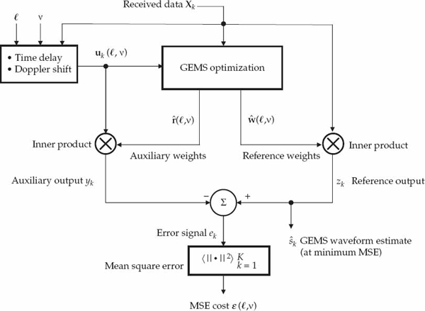
FIGURE 13.8 Flow-chart illustrating the GEMS algorithm. The procedure involves an optimization step that requires computing a closed-form solution for each input parameter setting over a bank of delays and Doppler shifts. Specifically, reference and auxiliary weight vectors are computed from a block of K input data vectors xk for each input value of and ν as the solution of a generalized eigenvalue problem. Spatial processing is performed to generate the mean square error (MSE) cost function ∈(, ν). In the single-source case, the GEMS waveform estimate may be extracted as the reference output at the delay-Doppler coordinates corresponding to the global minimum of the MSE cost function. In the multiple-source case, different waveform estimates may be extracted as reference outputs corresponding to the delay-Doppler coordinates of different deep local minima in the MSE cost function. © Commonwealth of Australia 2011.
• In the noiseless case, a non-trivial solution for υ yielding 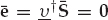 in Eqn. (13.62) exists if and only if the delay-Doppler displacement {, ν} matches the differential coordinates between a pair of modes (H1). Under H0, such a solution does not exist, and † = ||||2 > 0 for all υ ≠ 0.
• Under H1, the non-trivial solution for υ that satisfies in Eqn. (13.62) is unique up to a complex scale factor. This solution completely defines the set of all possible spatial filters {w, r} that respectively isolate the matched pair of modes.
• In the absence of noise, the spatial filters {w, r} spanned by this solution set will exactly recover a complex-scaled, time-delayed, and Doppler-shifted copy of the input sequence free of multipath which satisfies the processing objective.
• When noise is present, minimization of the error vector norm ||e||2 in Eqn. (13.88) with respect to the spatial filters {w, r}, and delay-Doppler displacement {, ν}, provides a basis for GEMS to blindly estimate the source waveform.
• The GEMS spatial filter ŵG optimizing this criterion function is used to derive the waveform estimate k in Eqn. (13.104). The auto-ambiguity function may be used to cue the GEMS procedure to the differential delay and Doppler between the two most dominant modes (as described shortly).
• While there are infinitely many spatial filters that can recover the source waveform in the noiseless case, the unique GEMS solution in the full-rank noise case attempts to reduce the noise contribution at the output as much as possible.
When multiple sources are present, it is necessary to interrogate more than one local minima in order to recover the different source waveforms. One approach is to interrogate all deep local minima of the GEMS cost function. Once the waveform estimates are extracted from each deep local minima, measures based on cross correlation analysis may be adopted to distinguish between waveform estimates corresponding to different sources, or different modes of the same source. This method clearly assumes that the different sources do not emit time-delayed and Doppler-shifted versions of a common waveform, as stated previously. Practical application of GEMS to the single- and multiple-source scenarios will be illustrated using experimental data in Sections 13.4 and 13.5, respectively.
13.3.3 Computational Complexity
This section analyzes the computational complexity of the GEMS algorithm relative to that of the classic (DOA-based) signal-copy procedure using the MUSIC estimator, which serves as a benchmark for comparison. Numerical examples are provided for the single-source case, where only the global minimum of the cost function needs to be interrogated for waveform recovery. However, the computational complexity calculations may be scaled accordingly to reflect different scenarios, including the multiple-source case, where a number of deep local minima need to be interrogated. The analysis is presented in a manner that allows the computational complexity of GEMS to be readily calculated for other practical situations of interest not limited to the examples provided in this section.
As the coordinates of the global minimum  of the cost function ∈(, ν) are not known a priori, a number of options are available in an operational system:
• Exhaustive Search: Evaluate ∈ (, ν) over a bank of delay-Doppler bins restricted to plausible values of (13.69). The granularity of the bins may be set to the sampling period Ts in delay and the FFT bins spaced by  in Doppler. In a time-invariant system, only a one-dimensional search in delay is required.
• Localized Search: For propagation channels with slowly-varying and smoothly evolving nominal mode parameter values (i.e., correlated changes in the nominal mode delay and Doppler coordinates), the search space may be narrowed for observation intervals subsequent to the first based on regions near the previously observed minima locations.
• Point Search: The auto-ambiguity function of the time-series output in a single receiver may be computed to estimate the locations of the mode differential delay-Doppler coordinates as the local peaks of this function, which may be used to cue the coordinates at which ∈(, ν) is evaluated.
The first option can be computationally expensive, depending on the number of receivers N, the extent of delay-Doppler domain to be searched, and the grid resolution used. The faster (third) option is to compute the auto-ambiguity function of the reference receiver output xk in Eqn. (13.105), where K′ = K − N. It is well known that |χ(, ν)| exhibits local peaks at values of the differential delay-Doppler offset between pairs of modes (Zhang, Tao, and Ma 2004). The global maximum of the ambiguity function occurs at the origin, while the coordinates of the next highest peak is expected at the differential delay-Doppler offset between the two most dominant modes. The coordinates of this second highest local peak in |χ(, ν)| may be used as the input to GEMS (i.e., to cue the GEMS procedure), as will be shown in the next section.

(13.105)
The computational complexity analysis for the single-source case is based on the point-search option, where the ambiguity function surface is used to cue GEMS to the coordinates of the global minimum. This represents a computationally efficient implementation of GEMS, as only one point in the cost function needs to be evaluated and interrogated for waveform estimation. The computational complexity may be readily scaled to account for the number of points evaluated in the cost function, as well as the number of deep local minima interrogated for waveform estimation. In other words, the elements of the analysis for the point-search option may be used to deduce complexity for other implementations.
A standard figure of merit for computational complexity is the number of complex multiplications (NCM). The complexity of the classic signal-copy procedure using the MUSIC DOA estimator is shown in Table 13.1. The study case numbers reflect the practical system parameters of N = 16, K = 125,000, and M = 2, which are relevant to the experiment described in the next section. The MUSIC spectrum is calculated over Nθ azimuths and Nϕ elevations with Nθ = Nϕ = 40. An N × N matrix inversion or eigen-decomposition is assumed to have an NCM of 4N3 in all comparisons. Table 13.2 shows the complexity for GEMS. By eliminating unnecessary computations (Zhang et al. 2004), and confining attention to the domain of uncertainty in {, ν}, the ambiguity function NCM is given by Eqn. (13.106), where an NCM of (N/2) log2 N is assumed for an N-point FFT. The numbers N = Nν = 40 mirror the values used in the experimental results of the following section.
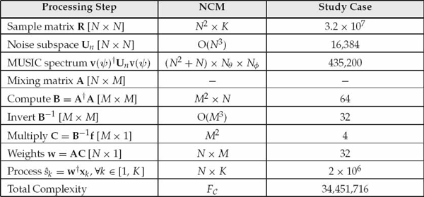
TABLE 13.1 Computational complexity of classic signal-copy procedure using MUSIC for DOA estimation. © Commonwealth of Australia 2011.
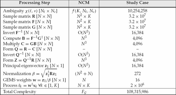
TABLE 13.2 Computational complexity of the GEMS waveform estimation algorithm. © Commonwealth of Australia 2011.
(13.106)
The GAM signal-copy approach cited previously requires the solution of a generalized eigenvalue problem (GEP) of small dimension at each DOA grid point, so it is computationally more expensive than MUSIC. For comparisons, the MUSIC DOA-based signal-copy procedure of lower complexity will be used as a benchmark. The relative complexity FR = FG/FC is defined as the NCM ratio of GEMS to that of the MUSIC DOA-based signal-copy procedure. As this figure varies with system parameters, FR is plotted as a function of K using different values of N in Figure 13.9a, and as a function of N using different values of K in Figure 13.9b. The main observation is that the complexity of GEMS is higher, but of the same order of magnitude as the classic signal-copy method over a wide range of system parameters.
The performance of this cued GEMS procedure relative to the DOA and GAM signal-copy methods will be illustrated using experimental data with known truth of the source waveform in the following section. Such comparison enables the tradeoff between waveform estimation performance and computational complexity to be evaluated for these different techniques in a real-world system. The computational complexity of GEMS will clearly be higher for multiple sources. In this case, changes in the relative complexity FR may be calculated by using the elements listed in Tables 13.1 and 13.2. An attractive feature of the GEMS algorithm is that the processing is highly parallelizable, such that the computational burden may be shared over multiple CPUs.
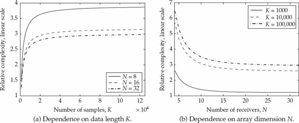
FIGURE 13.9 Relative complexity FR as a function of data length K and number of receivers N. © Commonwealth of Australia 2011.
13.4 SIMO Experiment
The main reason signal-processing techniques such as GEMS are developed is that they may be gainfully employed in practice. Numerical results in a simulation environment can provide useful insights regarding performance when it comes to comparing different techniques under controlled conditions. However, the critical question often raised by signal-processing communities relates to the effectiveness and robustness of different techniques in real systems. Despite the value of simulation studies, what is of ultimate concern to a user is how well the newly proposed techniques perform in practice, and what additional capability they can provide in actual systems with respect to traditional methods.
Although many signal-processing techniques have been successfully developed and tested on the basis of computer simulations, the path chosen here is to assess and compare the performance of GEMS against two benchmark signal-copy methods using real data acquired by an experimental HF system. By evaluating performance on real data collected in the field, this contribution complements the many existing works on blind waveform estimation by redressing the lack of experimental results available on this topic in the open literature.
13.4.1 Data Collection
Experimental data were collected by a well-calibrated two-dimensional (L-shaped) HF antenna array composed of N = 16 vertical monopole elements, spaced 8 m apart on each arm, with a digital receiver per element. This system was previously described in Chapter 10. The signal of interest (SOI) was received via the ionosphere from a source located at a ground range of 1851 km. The source transmitted a repetitive linear frequency modulated continuous waveform with center frequency fc = 21.620 MHz, bandwidth B = 10 kHz, and pulse repetition frequency fp = 62.5 Hz. Knowledge of the transmitted signal provides ground-truth information for assessing the estimation performance of different techniques that do not assume any prior knowledge about the source waveform. The receiving system acquired in-phase and quadrature (I/Q) components of the down-converted and baseband-filtered signals at a sampling rate of fs = 62.5 kHz. The data was collected continuously but processed as a sequence of coherent processing intervals (CPI) of To = 2-second duration.
By re-synthesizing the known reference signal, the channel-scattering function (CSF) resulting in the reference (first) receiver of the array is shown in Figure 13.10a as an intensity-modulated delay-Doppler display normalized by the maximum value. The received energy is dominated by M = 2 distinct propagation modes resolved at nominal time delays {τ1 = 6.54 ms, τ2 = 6.88 ms}. The Doppler spectra in Figure 13.10b are line plots taken from Figure 13.10a at time delays {τ1 = 6.54 ms, τ2 = 6.88 ms} to show the relative strengths and Doppler shifts of the two modes. The mode SNRs are in excess of 50 dB, but the SINR of mode 1 is only 6 dB when mode 2 is considered as the interfering multipath signal to be removed for waveform estimation. The two propagation modes also have different Doppler shifts {f1 = 0.3 Hz, f2 = 1.0 Hz} due to the different regular components of large-scale movement in the ionospheric layers responsible for signal reflection over the observation interval.
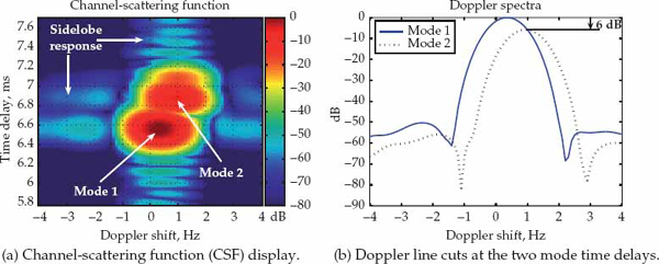
FIGURE 13.10 Location and relative strengths of the two dominant propagation modes resolved in the delay-Doppler plane. © Commonwealth of Australia 2011.
The normalized conventional spatial spectrum for the same CPI of data is shown in Figure 13.11a. The maximum value occurs at the azimuth and elevation {θ = 134°, ϕ = 18°}. The azimuth matches the known bearing of the source (134°), while the elevation (18°) is consistent with the angle expected based on geometrical considerations. However, the conventional spatial spectrum is not able to resolve the two modes in nominal DOA. Figure 13.11b shows the MUSIC spectrum for the same data assuming M = 2 signals. This spectrum is normalized by the maximum value, which also occurs at {θ = 134°, ϕ = 18°}.
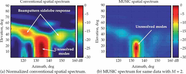
FIGURE 13.11 The two dominant modes cannot be resolved in nominal DOA by conventional beamforming and the MUSIC super-resolution technique. © Commonwealth of Australia 2011.
The two dominant modes cannot be resolved by MUSIC, even when the number of assumed signals is increased to M = 3 and M = 4 (not shown here). The inability to resolve the two modes is not only due to their closely spaced nominal DOAs, but also the departures of the mode wavefronts from the plane-wave model. The performance of super-resolution DOA estimation techniques is very sensitive to model mismatch, and consequently, so are the waveform estimation (signal-copy) procedures based upon them.
The wavefront distortions may be observed by resolving the modes in the delay-Doppler plane across all N = 16 receivers using the known reference waveform, as for the CSF. The mode wavefronts are extracted as the data snapshots received in the delay-Doppler bins corresponding to the peak coordinates of each mode, given by {τ1 = 6.54 ms, f1 = 0.3 Hz} and {τ2 = 6.88 ms, f2 = 1.0 Hz}. These snapshot vectors represent the mode wavefronts {am}m=1,2, which may be normalized to yield the mode spatial signatures  defined previously. The plane waves of best fit in a least-squares sense were found to have nominal DOAs of ψ1 = [θ1 = 134°, ϕ1 = 17°] and ψ2 = [θ2 = 134°, ϕ2 = 18°]. The multiplicative magnitude and phase distortions {dm}m=1,2 imposed on each mode relative to these plane waves of best fit are plotted as a function of receiver number in Figures 13.12a and 13.12b, respectively.
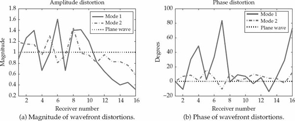
FIGURE 13.12 Complex-valued wavefront distortions received for modes 1 and 2 relative to the plane-wave model of best fit. © Commonwealth of Australia 2011.
Both the magnitude and phase deviate significantly with respect to the plane-wave model. In addition, the distortions are quite different for the two modes (i.e., propagation path dependent). The illustrated deviations from the presumed array steering vector manifold are the main reason why MUSIC fails to resolve the modes. Note that F{v1, v2} = 0.71, while F{v(ψ1), v(ψ2)} = 0.98, which implies that the mode spatial signatures are significantly further apart in N-dimensional space than the underlying plane waves of best fit. Hence, for techniques that do not rely on a manifold model parameterized by the signal DOA alone, the additional diversity in wavefront shape introduced by diffuse scattering provides greater opportunity to spatially resolve the modes. The nominal mode parameters listed in Table 13.3 were derived using the reference waveform, and represent ground-truth information for performance assessment in the analysis to follow.
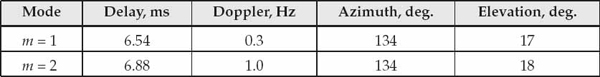
TABLE 13.3 Ground-truth information on nominal parameter values for propagation modes 1 and 2.
13.4.2 Signal-Copy Methods
In the case of spatially spread signals with non-planar wavefronts, a DOA estimation procedure can at best resolve and estimate the DOAs of the plane waves of best fit to the received spatial signatures. Although the nominal DOAs of the two dominant modes are not resolved by conventional beamforming or MUSIC, the plane waves of best fit extracted using the reference signal may be used to assess the performance of signal-copy procedures based on the plane-wave model. Reconstructing the mixing matrix using the plane waves known to be of best fit to the mode spatial signatures effectively provides an upper limit on the performance of any DOA-based signal-copy procedure for M = 2.
Setting Âdoa = [v(ψ1), v(ψ2)] and u1 = [1, 0]T in Eqn. (13.31) to preserve the first mode and eliminate the second mode yields the DOA-based signal-copy weight vector ŵdoa according to Eqn. (13.31). Figure 13.13a shows that an SINR improvement of 8 dB can be achieved at the output of the spatial filter ŵdoa with respect to that in the reference receiver. The choice to reject mode 2 in preference of mode 1 favors the DOA-based signal-copy procedure because this mode is more similar to a plane wave and is therefore canceled more effectively by the null at ψ2.
A GAM technique was also implemented for performance comparisons. The GAM approach in Astely et al. (1998) models the wavefront of a distributed signal as  where
where 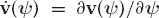 and ϑ is a free complex scalar parameter. A MUSIC-like spectrum may also be computed using the GAM model, but this technique is also unable to resolve the two modes. The potential effectiveness of the GAM method may be similarly assessed on the mode wavefronts extracted using the reference waveform. The GAM vectors {v(ψm, ϑm)}m=1,2 that provide the best least-squares fit to the extracted mode spatial signatures were computed, and the mixing matrix model Âgam = [v(ψ1, ϑ1), v(ψ2, ϑ2)] was substituted for A in Eqn. (13.31) to derive the GAM-based signal-copy weight vector ŵgam.
As shown in Figure 13.13b, the output of ŵgam provides a relative SINR improvement of 16 dB with respect to a single receiver. This is an additional 8 dB of SINR with respect to the traditional DOA-based signal-copy method. Such a substantial improvement testifies to the potential value of the GAM approach in a practical application. However, the mode to be rejected is still more than 25 dB above the noise floor. The reason the GAM method cannot provide a higher level of rejection is that such a manifold model is valid only for small angular spreads, whereas the distortions encountered in this application are large, and hence not accurately represented by the GAM model.
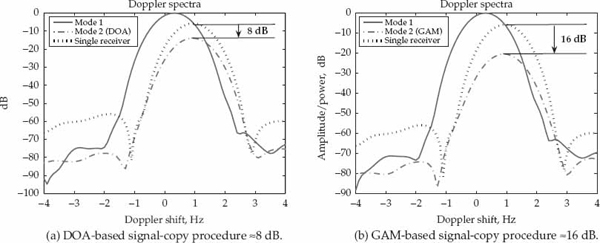
FIGURE 13.13 Doppler spectra showing improvement in output SINR resulting from the application of two benchmark signal-copy procedures relative to that in a single receiver. © Commonwealth of Australia 2011.
13.4.3 Application of GEMS
The application of GEMS is described in two parts. The first illustrates the capability of GEMS to blindly recover an accurate estimate of the source waveform that is contaminated by multipath. The second illustrates the capability of GEMS to estimate the crinkled wavefronts of the incident signal modes. Unlike the DOA- and GAM-based signal-copy methods, GEMS is applied in a strictly blind manner, i.e., without use of the reference waveform to estimate the mode spatial signatures. This represents a truly operational implementation of the GEMS algorithm.
13.4.3.1 GEMS Waveform Estimation
Figure 13.14a shows the cost function  (, ν) resulting for the GEMS algorithm, normalized by the maximum value over the search grid. The global minimum is located at {34 ms, 0.70 Hz}, which agrees well with the differential mode time delay τ2 − τ1 = 34 ms and Doppler shift f2 − f1 = 0.7 Hz using the values in Table 13.3. Figure 13.14b shows the normalized auto-ambiguity of the reference receiver output |χ(, ν)|/χ(0, 0), where the delay-Doppler coordinates of the highest peak (excluding the maximum at the origin) match the location of the global minimum in Figure 13.14a to the grid resolution. The coordinates of this peak
  are used to compute the GEMS weight vector ŵG for source waveform estimation.
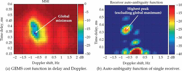
FIGURE 13.14 GEMS cost function showing location of global minimum, and auto-ambiguity function of a single receiver showing location of the second highest peak. © Commonwealth of Australia 2011.
Figure 13.15a shows that the SINR improvement at the output of ŵG is over 40 dB with respect to a single receiver, and 25 dB better than the GAM signal-copy method. Importantly, this substantial improvement has been obtained directly from the data in a strictly blind manner by the GEMS algorithm, i.e., without resorting to the known reference signal for resolving the modes in delay and Doppler. Hence, unlike the DOA and GAM signal-copy procedures, the results achieved by GEMS are a real improvement attained in practice, as opposed to an upper limit on performance.
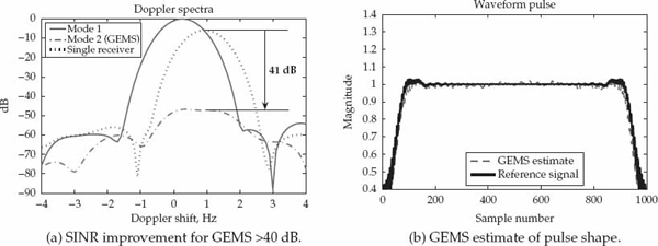
FIGURE 13.15 SINR improvement for GEMS, and a comparison of the waveform pulse shape estimated by GEMS with the known reference over 1000 A/D samples (16 ms). © Commonwealth of Australia 2011.
The impact on waveform recovery may be appreciated in Figures 13.15b and 13.16b, which compare the pulse shape of the known reference signal with those recovered by the three different estimation techniques. The GEMS estimate practically overlays the known reference in Figure 15.15b, while the benchmark signal-copy estimates exhibit signal envelope distortions due to residual multipath contamination in Figure 13.16b. Figure 13.16a shows the estimate resulting when the unit-norm non-triviality constraint ||[wT, rT]||2 = 1 is used instead of the GEMS constraint ||w†X||2 = 1 in Eqn. (13.88). The minimizing singular vector that arises for the former constraint attempts to cancel all signals and produces a very noisy estimate. This demonstrates the effectiveness of the GEMS constraint.
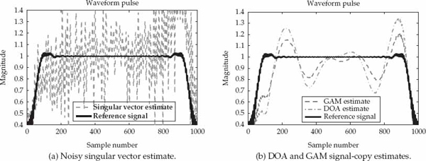
FIGURE 13.16 Comparison of the waveform pulse shape estimated using the singular vector method with those estimated using the DOA- and GAM-based signal-copy approaches. © Commonwealth of Australia 2011.
The reference ŵG and auxiliary  GEMS weight vectors are expected to separate the two modes, such that the earlier and later arrivals are isolated in the reference and auxiliary outputs, respectively. The CSF computed for the reference and auxiliary GEMS outputs are shown in Figures 13.17a and 13.17b, respectively. A comparison of these two displays with the CSF resulting for a single receiver in Figure 13.10a shows that the two modes have been effectively isolated by the spatial filters ŵG and . The earlier arrival appears at the output of ŵG, which is consistent with the expected performance of the technique. The removal of inter-mode contamination in each display of Figure 13.17 is quite remarkable, and confirms the practical effectiveness of GEMS for blind multipath separation.
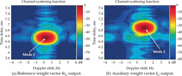
FIGURE 13.17 CSF outputs showing that the GEMS weight vector ŵG isolates mode 1 at the reference output, while  isolates mode 2 at the auxiliary output. Compare these results to the CSF display for a single receiver in Figure 13.10, where both modes are present in the output. © Commonwealth of Australia 2011.
An alternative visualization of the beneficial effect of multipath separation is presented in Figure 13.18, which shows the auto-ambiguity function (AF) of the GEMS waveform estimate compared to that of a single receiver output. The GEMS estimate in Figure 13.18b is consistent with the point-spread function of a repetitive linear FMCW waveform, while Figure 13.18a shows the deleterious effect of multipath in the single receiver output. Multipath causes significant “blurring” of the true point-spread function, and gives rise to a number of significant peaks that are well-separated from the main lobe. The poor quality of the resulting image in Figure 13.18a can significantly complicate the interpretation of the signal components present in the data based on the output of a cross-correlation receiver. With reference to these AF diagrams, the action of GEMS may be interpreted as the auto-focusing of a blurred image by virtue of multipath removal.
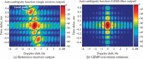
FIGURE 13.18 Auto-ambiguity function of a single receiver output and the GEMS waveform estimate. The former exhibits significant blurring due to multipath contamination, while the latter exhibits a well-focused point-spread function consistent with that of the transmitted source waveform. © Commonwealth of Australia 2011.
The single-source scenario is relevant to a number of practical applications, such as long-range HF communications and over-the-horizon passive radar (Fabrizio et al. 2009). In the latter case, an accurate estimate of the transmitted waveform from a source of opportunity is important for matched filtering (i.e., coherent range-Doppler processing). Such systems strive to minimize contamination due to multipath, such that matched filtering can be performed based on the source waveform point-spread function, as opposed to an inferior version that has been disturbed by multipath. The presence of multipath in the matching waveform may cause the detection of false targets in passive radar applications.
13.4.3.2 GEMS Wavefront Estimation
Once the mode waveforms have been separated using GEMS, it is possible to reconstruct an estimate of the signal matrix  defined previously. In the case of M = 2 dominant modes, the rows of ∈ CM×K are given by the outputs
  and
and  for k = 1, …, K, where ŵG and are the weight vectors extracted from the global minimum of the GEMS cost function. Based on the data model X = AS + N, and conditioned on the estimate , the least-squares estimate of the mixing matrix containing the mode wavefronts is given by  in Eqn. (13.107), where + = † (†)−1.
(13.107)
Estimates of the mode spatial signatures, denoted by  , are obtained by normalizing the columns of  as in Eqn. (13.108), such that
  . For example, consider the second mode m = 2, which has a more planar wavefront. Figure 13.19 compares the magnitude of the spatial signature estimated by GEMS for this mode as a function of receiver number with the measurements based on the reference waveform. The latter may be interpreted as true measurements of the mode wavefront structure. The GEMS estimate matches these measurements quite well across all N = 16 receivers.

(13.108)
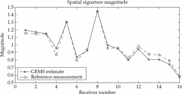
FIGURE 13.19 Receiver element comparison of the spatial signatures measured and estimated for mode 2 in magnitude. The reference measurements were extracted from the range-Doppler bin containing mode 2 after matched filtering is applied to each receiver using the known reference signal. The GEMS blind spatial signature estimate agrees well with the reference measurement. © Commonwealth of Australia 2011.
Results for the unwrapped phase of the same mode are compared in Figure 13.20, where the first receiver is used as the phase reference. The phase progression is quasi-linear over each arm of the L-shaped array, where the receiver numbers n = 1, …, 8 and n = 9, …, 16 form ULAs at right angles to each other. The mean slope of each quasi-linear phase progression depends on the nominal DOA of mode 2 with respect to the boresight of each arm. The GEMS phase estimates also agree well with measurements using the reference waveform. These wavefront estimates are useful for inferring the nominal DOA of modes that cannot be resolved on the plane-wave manifold (such as in the case of MUSIC). As demonstrated in the final section of this chapter, nominal mode DOA information may be used in conjunction with an ionospheric model to geolocate an HF source using a single ULA.
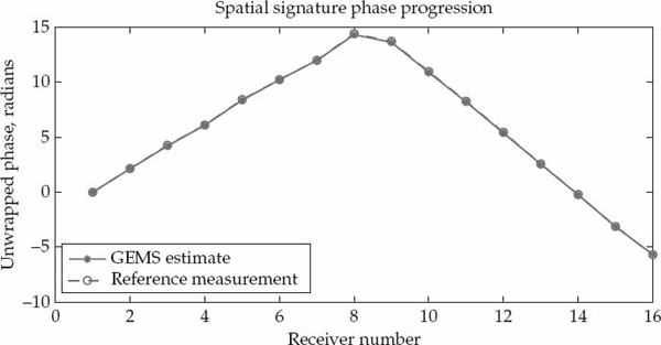
FIGURE 13.20 Receiver element comparison of the unwrapped phase across the two ULA arms of the L-shaped array for the spatial signatures estimated with GEMS and measured using the reference waveform. The phase estimates derived from GEMS agree well with reference measurements, and may be used to infer the nominal DOA of mode 2. © Commonwealth of Australia 2011.
13.4.3.3 CD and ID Wavefronts
Although GEMS is notionally based on the CD mode wavefront model, it was claimed in Section 13.3 that GEMS is robust to ID mode wavefronts, provided that sufficient spatial degrees of freedom are available. Earlier in this section, it was shown that GEMS blindly recovered accurate estimates of the transmitted source waveform and received mode wavefronts in a practical HF system. It is now of interest to investigate whether the two dominant modes present in the experimental data are better described by a CD or ID model. The wavefront planarity test proposed in Fabrizio et al. (2000a) may be applied to reveal the presence and characteristics of time-varying wavefront distortions over the processing interval for each mode.
Using the known reference waveform for range processing in each FMCW pulse, this test is based on the statistic defined by ρm(tp) ∈ [0, 1] in Eqn. (13.109), where ym(tp) is the array snapshot data vector extracted from range bin gm = cτm/2 containing mode m at pulse repetition interval tp = 1, …, P. In our case, we have that P = 125 for a 2-second CPI. Range processing allows the two dominant modes to be resolved into different group-range bins. This enables spatial signature variations to be analyzed over the different pulses in the CPI on a mode-separated basis.

(13.109)
The maximizing argument of Eqn. (13.109), denoted by ψm(tp), represents the DOA of the plane-wave model v(ψ) that best fits the received snapshot ym(tp) at pulse number tp. The value of ρm(tp) is a measure of how well the wavefront that is received from mode m matches the best fitting plane-wave at pulse number tp. A value near unity indicates an almost planar wavefront, while lower values indicate further deviation from the plane-wave manifold. Since the statistic ρm(tp) is invariant to the complex scale of ym(tp), it is agnostic to mode Doppler shifts. In other words, ψm(tp) and ρm(tp) are sensitive only to changes in the mode spatial signature. The CD model described previously is consistent with fixed values of ψm(tp) and ρm(tp) over the CPI, while variations with pulse number are expected for the ID model.
Figure 13.21 shows the profiles ρm(tp) resulting for the two modes m = 1, 2. The spatial signature of mode 1 is observed to deviate further from the plane-wave manifold than mode 2, which has a more planar spatial signature. The reasonably constant value of the profile for m = 2 indicates that this mode has a rather rigid wavefront over the CPI, i.e., more consistent with the CD signal model. On the other hand, the smooth variation of the profile observed for m = 1 indicates that the spatial signature of this mode is changing in a correlated manner over the CPI. This is more consistent with an (partially correlated) ID signal model. In other words, the multipath environment is in this case best described by a mixture of CD and ID modes. Such results indicate that modes reflected from physically well-separated regions in the ionosphere can exhibit wavefront distortions that have quite different structures and dynamic characteristics. The previous results on waveform estimation using the same data demonstrate the robustness of GEMS to the presence of an ID mode.
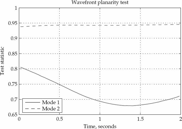
FIGURE 13.21 Example of wavefront planarity test statistic plotted for two simultaneously received modes over a 2-second CPI (125 PRI). The test indicates that mode 2 has a more planar and stable spatial signature over the CPI than mode 1. The spatial signature of the former is consistent with a CD model, while that of the latter exhibits greater temporal variation as is hence more aligned with the ID model. © Commonwealth of Australia 2011.
13.5 MIMO Experiment
A situation that is often of practical interest to wireless communication and radar systems involves the presence of multiple sources on the same frequency channel (i.e., co-channel sources). The different sources are assumed to be spatially separated such that propagation to the system occurs via nonidentical multipath channels. In this case the sensor array receives a convolutive mixture of the transmitted source signals. This was previously called a finite impulse response multiple-input multiple-output (FIR-MIMO) system. In mobile communications, it is desirable to separate and recover copies of the signals transmitted from multiple sources, whereas in active radar, the presence of independent co-channel sources may represent interference to be removed by the system.
Figure 13.22 schematically illustrates an FIR-MIMO system for Q = 2 sources. In this example, one source corresponds to the radar signal, while the other represents interference. Incidental interference due to co-channel sources is a common problem in the HF environment. This is mainly due to the dense occupancy of the HF band, and the ability of the ionosphere to propagate HF signals over very long distances (particularly at night when there is no D-region absorption).
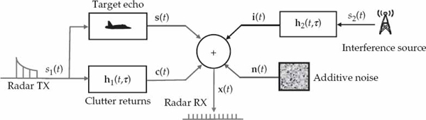
FIGURE 13.22 FIR-MIMO system illustrating the reception of two independent sources by an antenna array via different multipath channels. In this example, the first source s1(t) is a radar transmitter, which generates clutter and target echoes, while the second source s2(t) represents co-channel interference that is uncorrelated with the radar waveform. © Commonwealth of Australia 2011.
13.5.1 Data Collection
The L-shaped HF array described previously was used to simultaneously collect a number of different sources in the 62.5-kHz receiver bandwidth at a carrier frequency of 21.639 MHz. The spectrogram in Figure 13.23 shows a linear FMCW radar signal along side two AM radio signals acquired by a single receiver in the array. The different source transmissions occupy non-overlapping frequency channels to avoid mutual interference. For the purposes of this study, it is possible to superimpose two or more different signals onto a common center frequency. This creates a realistic co-channel source scenario for testing BSS techniques.
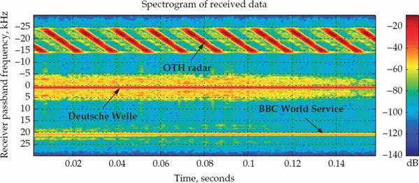
FIGURE 13.23 Sources in the receiver bandwidth include a linear FMCW radar signal, and two AM sources identified as BBC World Service and Deutsche Welle radio broadcasts. © Commonwealth of Australia 2011.
An FIR-MIMO system with Q = 2 sources was generated by digital down-conversion of the FMCW signal and BBC World Service broadcast to baseband and then superimposing the two received signals. This experimental technique avoids mutual interference, but effectively mimics the situation in which the two sources are present on the same frequency channel. Since the coherence bandwidth of the ionospheric channel is in the order of tens of kilohertz, this method faithfully replicates data that would arise for truly co-channel sources. GEMS and the classic signal-copy procedure are applied directly to the resulting AM-FM signal mixture.
For reference, the source emitting the linear FMCW was an HF radar, located at a ground range of 1851 km and bearing of 134° N with respect to the receiving system. The AM radio broadcast was from a BBC World Service station in Kranji, Singapore, located at a ground range of approximately 3400 km and bearing of 295° N from the receiver. As for the FIR-SIMO experiment, the data were collected continuously, but analyzed as a sequence of coherent processing intervals with 2-second duration.
13.5.2 Source and Multipath Separation
Figure 13.24 shows the MUSIC spatial spectrum for a particular CPI plotted as a function of azimuth θ and elevation ϕ assuming two signals. The DOA parameter vector is denoted by ψ = [θ, ϕ]. The two peaks occur at ψ1 = [134°, 19°] and ψ2 = [295°, 16°]. The azimuth estimates match the known FM and AM source bearings. However, multiple propagation modes could not be resolved in elevation by MUSIC when more signals were assumed (not shown here). This is partly due to the close spacing of the modes in elevation, and the poor elevation angle resolution of a ground-deployed array at near grazing incidence.
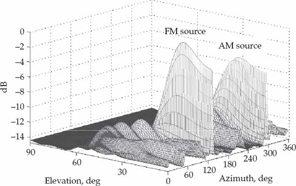
FIGURE 13.24 Two-dimensional MUSIC spectrum showing the azimuth and elevation of the FM and AM signals received by the L-shaped array. The different propagation modes of each HF source could not be resolved in elevation. © Commonwealth of Australia 2011.
Letting  where A = [v(ψ1), v(ψ2)] and u1 = [1, 0] leads to
 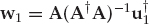 which yields the classic null-steering signal-copy weight vector for recovering the FM source waveform. The resulting estimate of this waveform
  is compared with the true source waveform, and the output of a single receiver, in terms of the pulse shape in Figure 13.25a. Although the null has reduced the corrupting effect of the AM signal on the FM source waveform estimate, significant distortion remains due to multipath interference as well as residual AM signal energy. Figure 13.25b shall be referred to in a moment.
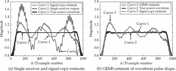
FIGURE 13.25 Comparison of the true FM waveform pulse shape with the estimates derived from a single receiver output, the classic DOA-based signal-copy procedure, and GEMS. © Commonwealth of Australia 2011.
Figure 13.26 compares the GEMS cost function for the FIR-SIMO and FIR-MIMO data. Figure 13.26a is a replica of the cost function shown previously for the FM signal only in Figure 13.14a. Figure 13.26b, plotted using a different time-delay scale, shows the cost function when GEMS is applied to the AM-FM signal mixture. Two deep local minima  are evident in the latter display. As expected, a minimum appears at the same coordinates as the global minimum in Figure 13.26a. This is labeled as “minimum 1” in Figure 13.26b, and is due to the FM source in the signal mixture. The application of GEMS to the FIR-MIMO system containing Q = 2 sources produces another deep local minimum, which is labeled as “minimum 2” in Figure 13.26b. This minimum is not related to the FM signal, but is formed due to the presence of the AM signal.
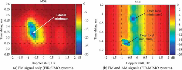
FIGURE 13.26 Comparison of GEMS cost functions arising for the single-source (FM only) and multiple-source (FM and AM) cases. The right-hand figure is plotted with a different time-delay scale to capture the second minimum. © Commonwealth of Australia 2011.
The GEMS weight vectors ŵG(q) corresponding to the minima  for q = 1, 2 were used to recover estimates of the associated source waveforms q(k) = ŵG(q)†xk. Figure 13.25b compares the GEMS estimate 1(k) and the DOA-based signal-copy estimate with the true source waveform. Clearly, the GEMS procedure yields a much more accurate waveform estimate than the classic signal-copy method. Indeed, the waveform recovered by GEMS exhibits minimal contamination and practically overlays the reference waveform.3
No ground-truth information is available to directly assess whether the GEMS waveform estimate 2(k) has recovered a copy of the AM source signal. The magnitude envelope of the estimated AM signal is shown as the solid line in Figure 13.27a. The dashed line in Figure 13.27a shows the auxiliary output formed as  , where
  is the auxiliary weight vector resulting at the minimum
  . At first glance, the reference and auxiliary outputs appear to be unrelated in Figure 13.27a.
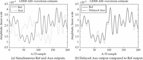
FIGURE 13.27 Magnitude of the reference and auxiliary GEMS waveform estimates for the AM source. In the figure on the right-hand side, the auxiliary output has been delayed by 0.88 ms (the location of the second minimum) to show the match between the two dominant propagation modes of the AM source. © Commonwealth of Australia 2011.
However, by delaying the auxiliary output a number of samples corresponding to the delay at which minimum 1 occurs (i.e.,  ), it is possible to compare estimates of the AM source signal carried by different propagation modes. Figure 13.27b shows a remarkable agreement between the amplitude envelopes of 2(k) and
  . It is evident that the two outputs are practically time-delayed replicas of one another, as expected for correct source and multipath separation. As these two outputs are derived from different spatial filters in the GEMS procedure, this result provides a high level of confidence that the AM source has also been estimated accurately in the presence of the FM source and multipath.
13.5.3 Radar Application
The question arises as to how the application of GEMS may provide a benefit in radar systems. To see this, consider a radar beam formed in the nominal direction of the AM interference source. A spectrogram of the resulting beam output is shown in Figure 13.28. The presence of the AM continuous wave (CW) signal and sideband components are clearly visible in the same frequency band as the FMCW radar signal. Two synthetic target echoes have also been injected, but are not distinguishable from the much more powerful AM and FMCW signals in Figure 13.28. These useful signals were injected at the receiver sample level (i.e., in the raw data prior to range processing and beamforming). The two synthetic targets have different ranges and Doppler shifts, but both are incident from the nominal direction of the AM “interference.”
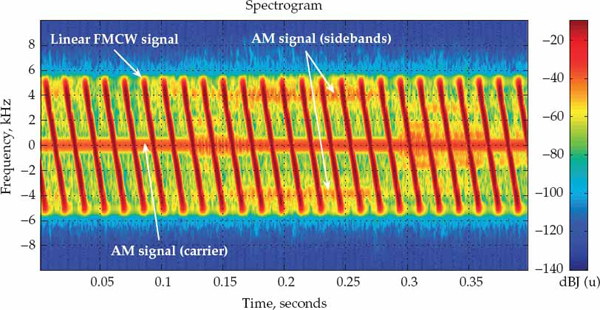
FIGURE 13.28 Spectrogram of the received AM source (BBC World Service) superimposed on the linear FMCW source from an OTH radar transmitter. © Commonwealth of Australia 2011.
Figure 13.29a shows the range-Doppler map resulting from the conventional beam output of Figure 13.28. The two strong direct-wave clutter peaks indicated in this figure correspond to the two dominant modes of the FMCW radar signal, which are clearly visible near zero Doppler frequency in the range-Doppler display. The powerful CW component of the AM signal manifests itself as a vertical “stripe” that is well-localized in Doppler frequency, but spreads over all range bins after pulse compression. On the other hand, the energy contained in the AM signal sidebands (i.e., the modulation component) is distributed over the entire range-Doppler map. In this case, both the CW and sideband components of the AM source mask the injected targets.
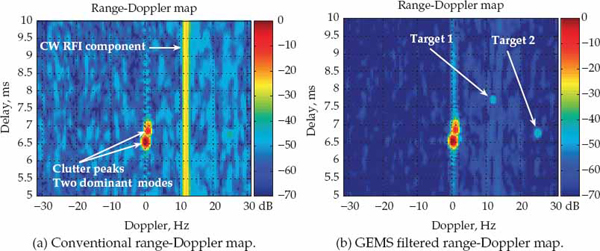
FIGURE 13.29 Conventional and GEMS-filtered range-Doppler maps for a main-beam interference scenario, where two synthetic targets have been injected in the nominal direction of the AM source. © Commonwealth of Australia 2011.
The AM source waveform is estimated using GEMS, as described in the previous section. The only exception is that GEMS is applied to the data containing the two synthetic targets, in addition to the AM and FM source signals, as required in an operational radar context. Once the time-series of the interfering AM signal modes are blindly separated and estimated using GEMS, these signal estimates may be complex-weighted and linearly combined so as to provide the best least-squares fit to the conventional beam output time-series in the pre-range (decimated) A/D sample domain.
This weighted combination of the recovered AM signal modes represents an estimate of the multipath interference that is received in the main lobe of the conventional beam. This estimate of the received AM interference signal may then be subtracted from the conventional beam output in an operation that may be loosely referred to as “‘waveform filtering.” Once the interference estimate has been subtracted from the conventional beam output in the pre-range sample domain, the remaining signal may be range-Doppler processed in the standard manner. The result of such processing is shown in Figure 13.29b, where the two synthetic targets are clearly distinguishable.
Figure 13.30 shows the range-bin line spectra containing the two targets before and after the GEMS-based waveform filter is applied for main-beam cancelation (MBC). The CW component has been canceled by about 40 dB in Figure 13.30a, while the signal sideband energy has been reduced by about 20 dB in Figure 13.30b. This is more than sufficient to unmask the target echoes, which were not detected by conventional processing. Note that the range-Doppler map in Figure 13.29b is relatively free of undesirable artifacts or “side effects” of such processing. This practical example also highlights the immunity of the approach to target self-cancelation and target-copying effects, which were discussed in Chapters 10–12.
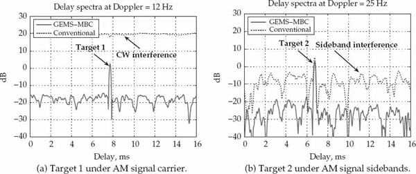
FIGURE 13.30 Range-bin spectra for the two synthetic targets before and after interference subtraction using the GEMS main-beam cancelation algorithm. © Commonwealth of Australia 2011.
In summary, the main strength of the developed GEMS technique resides in the mild assumptions made with regard to the mode wavefronts and source waveforms, viewed collectively, relative to other spatial processing methods for blind signal separation. This feature of GEMS broadens its scope for practical applications, and also increases its robustness to instrumental and environmental uncertainties that are inevitably encountered in real-world systems. In this sense, the GEMS algorithm represents an advance on current blind spatial-processing techniques for the problem considered.
13.6 Single-Site Geolocation
Thus far, relatively little attention has been paid to the use of channel information, which can also be blindly estimated along with the source waveform. The problem addressed in this section is that of HF single-site location (SSL), where it is required to estimate the geographic position of an uncooperative source located well beyond the line of sight from the signals received via the skywave propagation mode.
Much of the work in this area has focused around the use of two-dimensional apertures, which can unambiguously estimate both the azimuth and elevation angles of an incoming signal mode. A distinguishing aspect of the problem considered here is that geolocation of an unknown source is attempted using a receiving system based on a single ULA of antenna elements (with front-to-back directivity), where only the cone angle of an incoming signal mode can be measured.
A geolocation method that exploits multipath to resolve the “coning” ambiguity in a linear array is described and tested on real data in this section. Relative mode time-delay information extracted using the GEMS algorithm is also incorporated to make the approach robust in situations where the source is located near boresight. It is shown that by combining the cone-angle and time-delay information contained in all the multipath components opens up the possibility to perform meaningful HF-SSL using a linear array. The described method is also applicable to traditional HF-SSL systems based on two-dimensional apertures. However, the advantage in this case is reducing estimation errors, as opposed to resolving an ambiguity.
13.6.1 Background and Motivation
Figure 13.31 illustrates the classical HF-SSL concept, where a 2D aperture is used to measure the azimuth and elevation angles of the signal DOA. A real-time ionospheric model (RTIM) derived from a vertical incidence sounder (VIS) at the receiver site allows the elevation angle to be converted to a ground range for source position estimation. Table 13.4 compares the main characteristics of various geolocation methods. Trade-offs between the number of sites required, system complexity at each site, and knowledge demanded of the ionosphere and signal is summarized. A detailed description of HF-DF systems is beyond the scope of this chapter, but may be found in the authoritative texts of McNamara (1991) and Gething (1991).
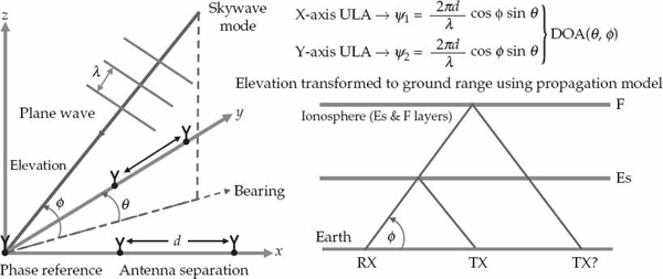
FIGURE 13.31 Classical HF-SSL concept illustrated for a 2D (L-shaped) array. Phase measurements made on both arms of the array yield two equations in two unknowns, such that the azimuth and elevation of the downcoming wave can be deduced. An ionospheric model is used to convert the elevation angle to a ground range based on the virtual height of reflection. © Commonwealth of Australia 2011.
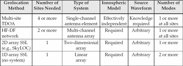
TABLE 13.4 Relative characteristics of different geolocation approaches. Reducing the number of sites tends to increase system complexity at each site, and increases reliance on knowledge of the ionosphere for propagation modeling. However, a redeeming feature of multi-channel array systems that use DOA as opposed to time-difference of arrival (TDOA) measurements for HF geolocation is that they are agnostic to the source waveform, which may be quite arbitrary. As far as HF-SSL systems are concerned, the last row signifies a reversal in the trend since system complexity is reduced from a 2D to 1D (linear) array. We shall see that it is possible to perform meaningful HF-SLL with a linear array provided that multipath is present, as indicated in the last column of the table. © Commonwealth of Australia 2011.
In particular, there currently appears to be no operational HF-SSL system based on a linear array. This is not surprising given that a linear array cannot estimate bearing and elevation independently due to the coning ambiguity. This section introduces and experimentally validates a geolocation method that exploits multipath to enable HF-SSL using a linear array. Such results have significant implications for implementing an HF-SSL capability on linear arrays existing in the field. Potential applications of this technology include search and rescue, enforcement of HF spectrum regulations, as well as in military situations McNamara (1991).
The key behind the approach is to simultaneously combine the cone angle and relative time-delay information contained in all of the signal modes received via skywave propagation from the source. This is in contrast to many current HF-SSL systems, which employ wavefront testing procedures (WFT) in order to produce valid estimates of the source position only at times of quasi uni-modal propagation (QUMP). This is tantamount to regarding multipath as a nuisance rather than an opportunity. Such systems not only miss the opportunity to use the additional information contained in the ensemble of paths, when considered jointly, but the severe pruning of data needed to satisfy QUMP conditions can also significantly limit the times at which measurements may be used.
For the purpose of this study, the HF-SSL system is assumed to be an antenna array connected to a multi-channel digital receiver system. Particular emphasis is on a ULA, but the described method is applicable to general array geometries with minor modification. In the ULA case, the antenna elements are assumed to have front-to-back directivity, such that the field of view is limited to ±90° from boresight. The source is assumed to be at relatively long range, such that propagation is via the skywave mode only. In other words, there is no reliance on the ground-wave mode, which is assumed to be highly attenuated. Ground waves can be useful for bearing estimation over short ranges, but its effective absence over long-range paths makes geolocation of an unknown emitter more challenging for a ULA.
The source of interest is assumed to emit an arbitrary waveform of finite bandwidth not restricted to a particular modulation format. The linear complexity of the waveform needs to exceed twice the maximum channel impulse response duration (as described previously for blind system identification in the context of identifiability). Importantly, propagation between the source and receiver is assumed to be via more than one ionospheric mode. Multipath propagation frequently occurs due to the E and F regions of the ionosphere, the presence of low- and high-angle rays, and magneto-ionic splitting that results in ordinary (o) and extraordinary (x) rays. Propagation via a single mode is the exception rather than the rule in this medium.
An RTIM is assumed to be available from a VIS at the receiver site. The quality of the ionospheric model may be improved by incorporating information from a network of spatially distributed ionosondes, or by using a backscatter sounder at the receiver site, for example. This is expected to be beneficial for long range paths, where the control point for the signal of interest is far from the receiver site. In this section, attention is restricted to path lengths less than 3000–4000 km. Range extents beyond this due to multi-hop ionospheric propagation will be considered in a future work.
13.6.2 Data Collection
Figure 13.32a shows the twin-dart antenna of the emitter to be geolocated in the experiment. This cooperative source was located near Broome, on the north-west coast of Australia. Figure 13.32b shows the receiving ULA of the east arm of the Jindalee Operational Radar Network (JORN) OTH radar, located near Laverton in western Australia. This ULA has an aperture of 2970 m and consists of 480 twin-monopole (end-fire) elements with a digital receiver per element. The geometry of the experiment is illustrated in Figure 13.33a. We shall refer back to Figure 13.33b in due course.
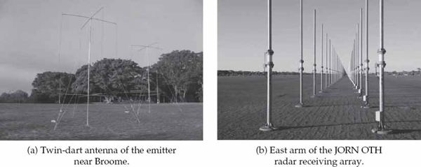
FIGURE 13.32 Pictures of the twin-dart antenna used to emit the test signal from a site near Broome, Western Australia, and the east arm of the receiving uniform linear array of the JORN OTH radar at Laverton, Western Australia. © Commonwealth of Australia 2011.
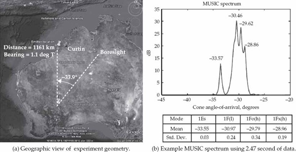
FIGURE 13.33 Experiment geometry showing emitter ground range and bearing relative to the receiving ULA position and boresight direction. An example of MUSIC spectrum showing the estimated mode cone angles is also shown along with the mean and standard deviation of measurements averaged over a 1 minute interval of data.
The emitter is located at a ground distance of 1161 km from the receiver site with a great circle bearing of 1.1°N. The bearing of the source is −33.9° relative to the ULA boresight direction. Figure 13.34a shows an ionogram recorded by the VIS system at the receiver site, while Figure 13.34b shows an oblique incidence sounder (OIS) ionogram recorded for the Curtin-Laverton path. The location of Curtin is indicated in Figure 13.33a. A multi-segment quasi-parabolic (QP) ionospheric profile model was manually fitted to the VIS and OIS ionograms. The fitted model parameters are indicated in the two figures showing the VIS and OIS ionograms, respectively.
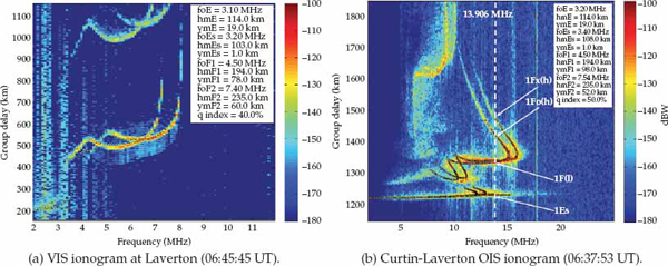
FIGURE 13.34 VIS ionogram at Laverton (06:45:45 UT) and Curtin-Laverton OIS ionogram (06:37:53 UT). The QP ionospheric model parameters manually fitted to each ionogram are listed in the figures. © Commonwealth of Australia 2011.
The source emitted a narrowband waveform with flat spectral density. The carrier frequency was 13.906 MHz and the bandwidth was 8 kHz. A spectrogram of the waveform is shown in Figure 13.35. Although the source was cooperative, the signal waveform was assumed to be unknown. The received signal was digitally down-converted and decimated to a sampling frequency of 31.25 kHz. The array data were acquired in consecutive processing intervals of approximately 2.5-s duration. This experiment was performed on 18 August 2011 starting at 06:48 UT (14:48 local time).
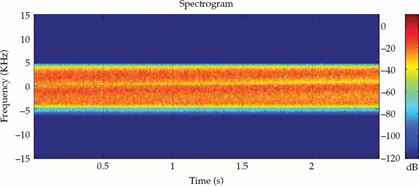
FIGURE 13.35 Spectrogram of the source signal with a bandlimited spectral density. No knowledge is assumed regarding the modulation format of the emitted waveform. © Commonwealth of Australia 2011.
Figure 13.34b shows that four ionospheric modes are resolved in the OIS trace for the Curtin-Laverton path at 13.906 MHz. These single-hop modes are sporadic-E “lEs,” the F-layer low-angle ray “1F(l),” and the F-layer high-angle rays, namely, the ordinary wave “1Fo(h)” and extraordinary wave “1Fx(h).” The reader may refer to Chapter 2 for an explanation of low/high rays and o/x waves. The OIS path midpoint is about 86 km from the control point of the source-to-receiver path. This is considered to be a short distance on the spatial scale of ionospheric variability. However, the ionogram was recorded approximately 10 minutes prior to the source, which may be a significant interval on the temporal scale of ionospheric variability. On the other hand, the VIS was recorded less than 3 minutes earlier, but the control point for the source is about 586 km from the VIS.
13.6.3 Geolocation Method
The geolocation method is composed of three elements. The first makes use of phase measurements across the antenna elements in the array, from which the cone angles of the different signal modes can be estimated. A cost function that combines the phase measurements associated with the cone angles of all signal modes with predictions based on an ionospheric model may be used to obtain a position fix on the source. However, such a method is only applicable for sources with a bearing that is not near or at boresight. To address this issue, inter-mode TDOA information extracted using the GEMS technique is incorporated for range estimation, as the second component. The third component of the introduced geolocation method fuses the mode spatial phase and time-delay information to estimate the source position.
13.6.3.1 Phase Measurements
Define  as the array snapshot vector recorded at time sample k = 1, …, K starting at receiver s = 1, …, N − Ns + 1, where Ns and N are the number of elements in the subarray and array, respectively. To be clear, the subarray refers to a selected number Ns < N of adjacent receivers in the full array. Compute R as the spatially smoothed sample spatial covariance matrix by forward-backward averaging in Eqn. (13.110), where J is the exchange matrix with ones on the anti-diagonal (Pillai 1989). The symbols T, ∗, and † denote the transpose, conjugate, and Hermitian (conjugate-transpose) operators, respectively.

(13.110)
The mode cone angles may be estimated using the MUSIC algorithm based on the eigen-decomposition of R in Eqn. (13.111), where Qs and Qn represent the signal and noise subspaces, respectively. Sub-aperture smoothing trades off robustness for correlated multipath arrivals against spatial resolution. Here, N = 480 and Ns = 240 was used as a compromise between the two competing objectives. The number of modes is determined as M = 4 in the following, so Qn contains the Ns − M eigenvectors with the smallest eigenvalues (Schmidt 1981).
(13.111)
The MUSIC spectrum is computed as p(ψ) in Eqn. (13.112), where v(ψ) = [1, e jψ, …, e j (N−1)ψ]T is the ULA steering vector.4 As illustrated in Figure 13.31, the phase ψ = 2πd sin φ/λ, where sin φ = cos ϕ sin θ for a ULA on the x-axis, and φ is the cone angle. The MUSIC spectrum resulting for a 2.47-second interval of data is illustrated in Figure 13.33b. The estimated cone angles  associated with the four (m = 1, …, M = 4) dominant peaks are labeled in this figure.

(13.112)
This process may be repeated over successive processing intervals to obtain an average estimate of the mode cone angles. The table in Figure 13.33b shows the mean and standard deviation of the cone-angle estimates using one minute of data. Cone angles closer to boresight are associated with modes reflected from greater virtual heights. The estimated phases  can be arranged into the measurement vector
  in Eqn. (13.113), where
  .
.
(13.113)
For a hypothesized source ground range R, and great circle bearing θ, the ionospheric model can be used to predict a phase angle ψm(R, θ) for each propagation mode. These predictions were derived using analytical ray tracing and virtual ray path geometry principles assuming a spherically symmetric QP profile. The effect of ionospheric gradients or tilts on geolocation accuracy is less pronounced on long-range paths than it is on short-range ones. Neglecting tilts, the model predictions may be arranged into the vector ψ(R, θ) in Eqn. (13.114), where ψ1(R, θ) < ψ2(R, θ) < … < ψM(R, θ).
(13.114)
Even when ionospheric tilts can be ignored, and the cone angle furthest from the boresight direction (i.e., 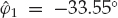 in this case) is correctly associated with the sporadic-E propagation mode, it is still not possible to obtain a unique fix on the source position using a single mode from a linear array. This is because there is a continuous locus of source range-bearing pairs on the ground that give rise to the same cone angle. This ambiguity is illustrated for in Figure 13.36a. The true source location is indicated by a black dot. Figures 13.36 and 13.37, in the same format, illustrate the ambiguities for the other estimated cone angles on a mode-by-mode basis.
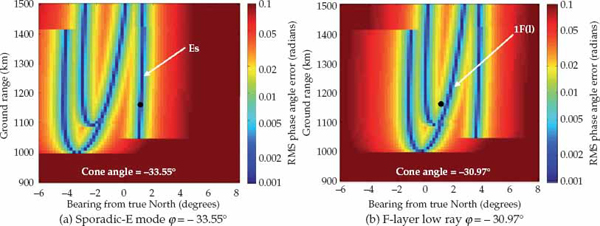
FIGURE 13.36 Loci of ambiguity in the range-bearing plane associated with the cone angles estimated for the sporadic-E and F-layer (low-ray) modes, denoted by the abbreviations 1Es and 1F(l), respectively. © Commonwealth of Australia 2011.
FIGURE 13.37 Loci of ambiguity in the range-bearing plane corresponding to the cone angles estimated for the ordinary and extraordinary high angle rays in the F-region, denoted by the abbreviations 1Fo(h) and 1Fx(h), respectively. © Commonwealth of Australia 2011.
The main point is that it is not possible to resolve these ambiguities when the phase measurements for each mode are considered separately and processed on an independent basis. These ambiguities can be resolved by jointly processing the phase measurements made on different modes, i.e., by exploiting multipath to estimate the source position. Specifically, the RMS phase error cost function in Eqn. (13.115) may be proposed, where  is the error vector between the measurements and model.
(13.115)
The source position may be estimated by evaluating cψ(R, θ) over a grid of candidate range-bearing tuples, and observing the coordinates of the minimum, i.e., where the phase measurements best fit the model predictions in a least-squares sense. The cost function evaluated using real data is shown in Figure 13.38a. The estimated and true source locations are also indicated in Figure 13.38a. In this example, the geolocation error is 25.8 km over a 1161 km ground distance path. Based on skywave propagation only, and the use of a single receive site, this is considered to be a new result for HF source geolocation with a ULA.
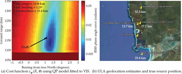
FIGURE 13.38 Cost function cψ(R, θ) using the QP ionospheric model fitted to VIS ionogram, and geographic map showing the geolocation estimates relative to true source position. © Commonwealth of Australia 2011.
13.6.3.2 Delay Measurements
A potential problem with using cψ(R, θ) in isolation is that there is effectively no coning for a source near boresight. In this case, the cost function elongates in range such that only bearing estimation becomes possible. To overcome this limitation, it is proposed to incorporate an inter-mode TDOA method for range estimation. The relative mode time delays may be estimated by cross-correlation analysis when the source waveform has a known parametric form, e.g., linear FMCW. The problem is how to estimate the mode differential time delays for an unknown source that emits an arbitrary waveform. The previously introduced GEMS algorithm is used here to estimate the differential mode time delays.
Figure 13.39 shows the GEMS cost function computed using the same 2.47-second processing interval of data as in Figure 13.33. A total of  minima are expected,5 excluding the trivial solution at the origin. The cost function exhibits Q = 6 minima, which corresponds to M = 4 modes, as predicted from the OIS ionogram in Figure 13.34b. The location of the minima are also listed in Figure 13.39. Importantly, GEMS exploits wavefront “crinkles” caused by diffuse scattering to resolve modes with similar or the same nominal DOAs. This enables GEMS to resolve sources near or at boresight.
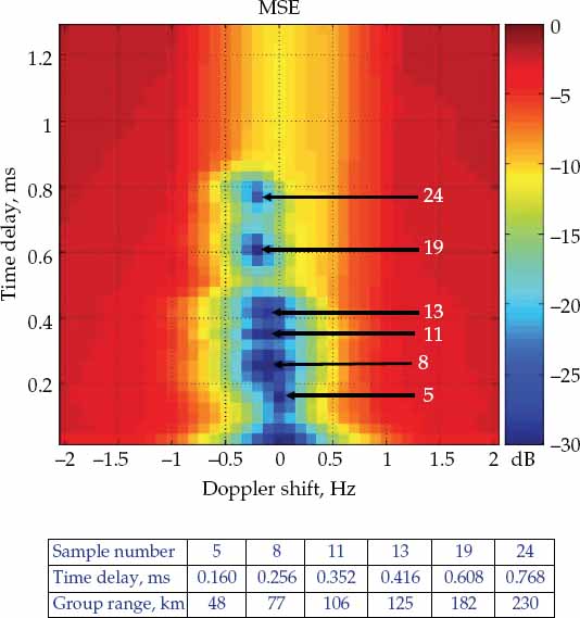
FIGURE 13.39 GEMS cost function in the differential delay-Doppler plane. © Commonwealth of Australia 2011.
The differential group-range estimates of the modes, denoted by  q, may be arranged into the measurement vector
  = [1, …, Q]T, such that 1 < 2 < … < Q. Similarly, the ionospheric model may be used to predict the differential group ranges arising between different pairs of modes as a function of the hypothesized source ground range and bearing. The resulting model predictions, denoted by gq (R, θ), are assembled in ascending order to form the vector g(R, θ) in Eqn. (13.116).
(13.116)
The RMS group-range cost function may then be computed as cg(R, θ) in Eqn. (13.117), where the error vector is εg(R, θ) = g(R, θ) − . This function is very weakly dependent on bearing due to the impact of the Earth’s magnetic field on signal propagation through the ionosphere. Figure 13.40 shows the representative range-only dependence of cg(R, θ), which is more or less the same for all bearings.
(13.117)
The top panel in Figure 13.40 shows the differential group ranges measured using GEMS as horizontal dashed lines. The model predictions for each mode pair combination are plotted against source ground range as solid lines. The cost function cg(R, θ) is shown as a function of source ground range in the bottom panel of Figure 13.40. The minimum occurs at a range of 1195 km, which corresponds to a range error of 34 km. This ground range estimate of the source location has been obtained using inter-mode TDOA information obtained at a single site for a far-field source that emits an unknown waveform. This is also regarded as a new result for HF-SSL.
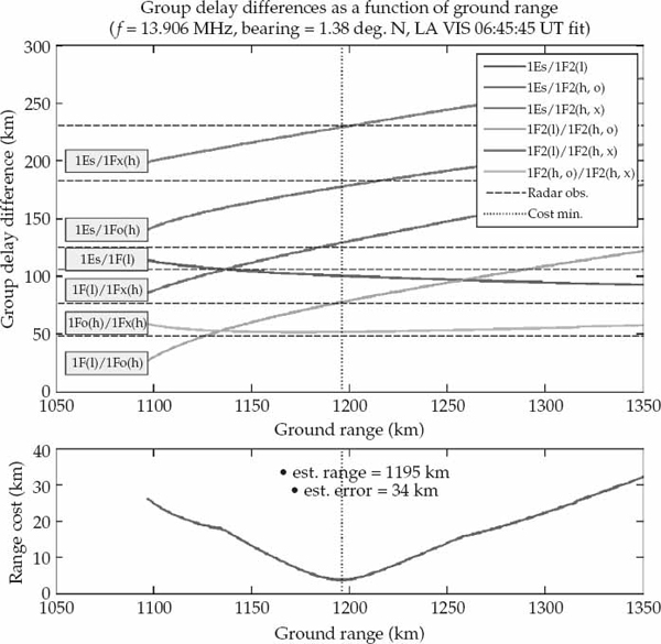
FIGURE 13.40 Cost function cg(R, θ) used to estimate the source ground range.
13.6.3.3 Fused Measurements
The phase-only and group-range cost functions may be fused to take advantage of the relative benefits that each provides. A possible way to fuse the cost functions is to express the phase rms error cψ(R, θ) as a bearing rms error cθ(R, θ) using standard transformations, and to compute the cross-range rms error as Rcθ(R, θ). The down-range rms error is well-approximated by cg(R, θ). Hence, the rms Euclidean distance error may be approximated as c(R, θ) in Eqn. (13.118).
(13.118)
Figure 13.41a shows a plot of c(R, θ) with the estimated and true source positions indicated. When the QP model fitted to the VIS is used, the geolocation error is 32.3 km. Figure 13.41b shows that this error reduces to 15.7 km when the ionospheric model fitted to OIS record is used instead. Figure 13.38b shows the true and estimated source positions on a geographic map zoomed into the Broome area.
(13.119)
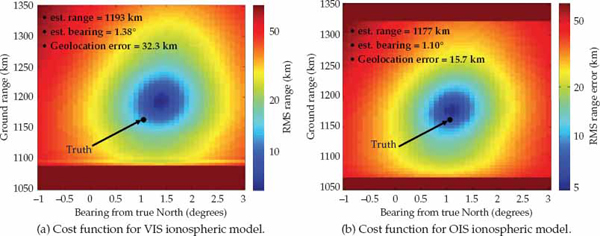
FIGURE 13.41 Fused cost function c(R, θ) based on QP ionospheric models fitted to the VIS and OIS ionograms. © Commonwealth of Australia 2011.
The estimate resulting for another OIS ionogram recorded later at 06:52 UT (with 17.2 km geolocation error) is also shown to indicate the robustness of the approach. It is emphasized that these accuracies should be interpreted as preliminary results only, rather than upper bounds on achievable geolocation performance. It is envisaged that a number of refinements can be made to the geolocation technique to reduce source position estimation errors to around 10 km; see Fabrizio and Heitmann (2013). Some topics for future work are discussed below.
13.6.4 Summary and Future Work
An HF-SSL method for the geolocation of long range sources propagated exclusively via skywave paths has been proposed and experimentally validated on a ULA. The technique is essentially agnostic to the class of waveform emitted by the source and exploits the geometrical relationships satisfied by multipath propagation to resolve the inherent coning ambiguity of a ULA.
By incorporating all multipath measurements and the physical constraints associated with such propagation into the cost function, the introduced HF-SSL procedure allows the source position (and mode group ranges) to be estimated. This multipath-driven HF-SSL method represents a fundamentally new approach to HF geolocation.
Experimental trials confirm the validity of the approach, which combines both cone angle and TDOA information for all resolved propagation modes. The described approach is also applicable to two-dimensional receiver apertures with minor modification. In this case, the main advantage is expected to be estimation error reduction as opposed to resolving an ambiguity.
Besides the aforementioned practical applications of HF geolocation, the approach is also of interest for the inverse problem of estimating the signal virtual reflection heights when the position of an uncooperative source is known. The ability to estimate mode structure for a known path using emitters of opportunity that probe ionospheric control points in regions which cannot be monitored by dedicated sounders is desirable for coordinate registration in OTH radar systems. The estimation of ionospheric tilts when the source position is known is a subject of current investigation.
Future work involves performance analysis as a function of receive aperture length, mode signal-to-noise ratios, waveform bandwidth, and source distance. Extensions to the approach include the incorporation of known reference points (KRPs) when available, numerical ray tracing (NRT) through an RTIM derived from a network of ionosondes (for long ranges), ionospheric tilt correction (for short ranges), time averaging of estimates, and refinement of the cost function expression to account for ionospheric uncertainty, including the weighting of different mode contributions. It is anticipated that a multipath-driven estimation approach may also be useful in other systems, not limited to HF or electromagnetic signals.
____________________
1 The term “clairvoyant” implies that the signal mixing matrix A is known a priori.
2 In the case of signal modes with widely separated nominal DOAs (i.e., beyond the Rayleigh resolution limit), the presence of wavefront distortions also has the potential to degrade performance.
3 The transmitted FM signal is tapered in amplitude at the edges of the pulse to reduce out-of-band spectral emissions.
4 The angle ψ is defined here as the phase difference between adjacent antenna elements in the ULA for a plane wave incident from azimuth θ and elevation ϕ.
5 The definition of Q stated in this section is not to be confused with its previous definition as the number of sources.
..................Content has been hidden....................
You can't read the all page of ebook, please click here login for view all page.