
3.3 Frequency Management
The performance of skywave OTH radar systems is strongly influenced by the choice of operating frequency. The optimum choice of carrier frequency for a particular mission type and surveillance region location depends strongly on the prevailing HF signal-plus-noise environment and ionospheric propagation conditions. Specifically, deviations from the optimum carrier frequency in the order of hundreds of kilohertz can significantly affect the quality of skywave propagation (SNR and/or SCR). On the other hand, differences of a few kilohertz can substantially change the level of interference received from other narrowband users of the HF spectrum. System performance is not only sensitive to relatively small departures from the optimum carrier frequency, but also to waveform design and parameter selection. It follows that a poor choice of operating frequency and waveform can lead to serious degradations in target detection and tracking performance.
Statistical descriptions of the ionosphere based on extensive analysis of historical data gathered at different sites around the world can be used to predict monthly median propagation conditions for a particular skywave circuit and time. The question arises as to the utility of these empirically derived climatological models for guiding OTH radar operation. In practice, it is found that the random variability of actual ionospheric conditions with respect to median predictions is significant enough to cause poor performance of OTH radar systems. Statistical forecasts based on climatological models need to be supported by real-time and site-specific HF propagation information for more effective OTH radar operation.
To optimize the selection of carrier frequency and waveform parameters, it is considered imperative for an OTH radar system to incorporate a suite of auxiliary sensors that can evaluate ionospheric propagation conditions and monitor spectral occupancy at the time of operation from the radar site(s). In other words, the requirement is for a real-time and site-specific frequency management system (FMS) that provides OTH radar operators with high-fidelity advice to select the most suitable carrier frequency and waveform parameters for the mission at hand. The amount of operator intervention needed in this process may be reduced by incorporating a control system to interpret the sensor data and automatically configure radar operations based solely on mission requirements.
The techniques used for optimum frequency selection in OTH radar differ markedly from those used in point-to-point HF communication systems. This is because the metrics used for OTH radar frequency selection, such as signal-to-noise ratio, Doppler spectrum contamination, and multi-mode content, have relative priorities that change depending on the target class of interest. Another factor that influences frequency selection for OTH radar is need to simultaneously illuminate a large surveillance region rather than a localized area. As the value of each performance metric changes as a function of frequency, time, and location, optimum frequency selection for OTH radar would be time-consuming for operators in the absence of an automated FMS.
High-fildelity propagation-path information is also required to accurately transform radar coordinates to geographic position to produce ground-registered radar tracks. Besides the real-time uses of FMS data products in an operational OTH radar system, off-line analysis of synoptic environmental data archives that routinely accumulate calibrated measurements (even when the radar is not operating), may be used to derive quantitative estimates of radar performance which are valuable for guiding future system design.3 This is recognized as another important role of the FMS.
This section briefly overviews the main characteristics of the FMS originally conceived for the Jindalee OTH radar in Earl and Ward (1986). The first part of this section describes the backscatter sounder and mini-radar systems, which provide information regarding signal power and Doppler spectrum characteristics for propagation-path assessment, respectively. The second part describes the spectral surveillance and background noise monitors, which identify clear frequency channels in the HF band and measure the environmental noise spectral density in different directions, respectively. Vertical/oblique incidence sounders and channel scattering function equipment, which provide detailed information on multimode-propagation structure, are discussed in the third part of this section. The reader is referred to Earl and Ward (1986) or Earl and Ward (1987) for a detailed description of the Jindalee OTH radar FMS.
3.3.1 Propagation-Path Assessment
Due to the vast coverage of OTH radar (millions of square kilometers), it is impractical to perform ionospheric propagation-path assessments over the entire search area by relying on point-to-point (vertical and oblique) ionospheric sounders alone. The large number of ionospheric control points that need to be monitored would require a dense ionosonde network, which may be prohibitive from a cost perspective. Moreover, the remote locations of many control points in the coverage often makes it infeasible or inconvenient to install and maintain such systems, particularly beyond sovereign coastlines or borders.
The technique used to measure the signal power density that is propagated by the ionosphere to a remote location and then scattered from the Earth’s surface back along a similar path to a receiver located at or close to the transmit site is that of backscatter sounding (BSS) (Croft 1972). In the two-site (quasi-monostatic) configuration, the BSS transmit and receive subsystems are colocated with those of the main OTH radar facility to provide site-specific measurements of the backscattered signal power density in the form of an ionogram. The BSS ionogram is essentially a measure of the signal power density backscattered from land and sea surfaces (as well as other scatterers) in the coverage area as a function of beam direction, group-range, and operating frequency. This in turn provides a quantitative indication of the signal power density that illuminates targets in a surveillance region of the main radar at different operating frequencies. The power density of the illumination is not directly observable in this process due to the unknown backscattering coefficient of the Earth’s surface.
The backscatter sounder provides an assessment of the propagation conditions in terms of the returned signal power. Combining this information with background noise spectral density measurements made at the same site allows frequency channels to be ranked in terms of SNR at a particular time and for a particular surveillance region. SNR is the primary performance metric for the detection of fast-moving targets (e.g. aircraft). However, the BSS ionogram does not provide any information about the spectral characteristics of the backscattered echoes. Propagation-path assessment in terms of clutter Doppler spectrum contamination is of primary importance for the detection of slow-moving targets (e.g., ships). For this reason the FMS includes a low-power frequency-agile miniradar system to measure the spectral characteristics of the received signal. The key features of the backscatter sounder and miniradar system used for skywave propagation-path assessment are described below.
3.3.1.1 Backscatter Sounder
Backscatter sounding represents an efficient technique for gaining an overall appraisal of propagation conditions over a wide area from the OTH radar site(s). In the Jindalee OTH radar system, a single vertical LDPA antenna element located at the transmitter site (Harts Range, approximately 100 km to the northeast of Alice Springs, central Australia) is dedicated to the FMS and used to floodlight the entire OTH radar coverage area to the northwest of Australia. At the receiver site (Mt. Everard, approximately 20 km to the northwest of Alice Springs), a ULA of 28 dual-fan elements are used to feed a beamformer, resulting in the generation of eight receiver beams contained within the (approximately 90-degree) arc of the FMS transmit beam.
The transmitted linear FMCW sweeps up at a rate of 100 kHz/s, such that it takes 4 minutes to record an ionogram between the frequency limits of 6 and 30 MHz for all of the eight FMS beams. Specifically, the received signal power is measured as a function of propagation delay at 200-kHz frequency increments with a group-range resolution of approximately 50 km and a group-range coverage of up to 10000 km. Note that each 200 kHz increment is used to obtain multiple estimates of the clutter power-delay profile on all 8 beams using an effective signal bandwidth of 3 kHz.4 The long (multi-hop) distance coverage of the backscatter ionogram is useful for identifying potential sources of clutter that may fold into the OTH radar surveillance region through first- and higher-order range ambiguities. This assists the radar operator to select an appropriate waveform PRF.
Figures 3.27a and 3.27b show two backscatter ionograms recorded simultaneously by the Jindalee FMS at 19:42 LT on two beams spaced approximately 45 degrees apart. The differences between the received signal power distributions in group-range and frequency, particularly at long distances in this example, clearly demonstrates the azimuthal dependence of propagation conditions. Figure 3.28b shows a morning ionogram recorded in the same beam as the evening ionogram in Figure 3.28a. The differences between these two ionograms illustrates the significant time-of-day dependence of skywave propagation. Some more detailed features of the illustrated BSS data examples will now be discussed.

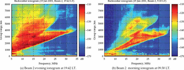
The increase in minimum group-range of received signal backscatter with operating frequency gives rise to a so-called “leading edge,” which is labeled in Figure 3.27a. This feature is typical of F-region propagation. In this nighttime example, only the F2-layer affords skywave propagation above 10 MHz and effectively no backscatter is received at group-ranges prior to the leading edge at a particular frequency. In this case, the leading edge of the F2-layer in the BBS ionogram represents the skip-distance measured in group-range as opposed to ground-range along the FMS beam direction. For a given group-range, enhanced illumination and hence backscatter due to ionospheric focussing occurs at the frequency which places the group-range immediately beyond the skip-zone. As illustrated in Figure 3.27a for a hypothetical surveillance region with a group-range extent of 2000–3000 km, the strongest backscatter is received at a frequency near 18 MHz in the direction of beam 2. In Figure 3.27b, this frequency is about 17 MHz for a surveillance region with identical group-range extents but shifted approximately 45 degrees in azimuth.
Figures 3.27a and 3.27b also show that significant clutter power is returned from long-distances via multi-hop skywave paths and possibly trans-equatorial propagation modes. Typical nighttime PRFs used for aircraft detection may lie between 30 and 50 Hz, which have first-order group-range ambiguities of 5000 and 3000 km, respectively. If the selected PRF has a group-range ambiguity that coincides with strong backscatter, potentially Doppler-spread clutter can fold into the surveillance region and obscure target echoes. It is evident from Figures 3.27a and 3.27b that the same choice of PRF can lead to strong range-folded clutter in the direction of beam 6 but not in that of beam 2. In this case, both the carrier frequency and waveform PRF need to be adjusted depending on the direction of the surveillance region.
Figure 3.29 shows the backscattered signal power received as a function of group-range for two different operating frequencies and beam directions at a particular time. The example in Figure 3.29a shows that the range region of strong backscatter power, which starts immediately beyond the skip-zone, moves out in group-range from roughly 1000 km to 2000 km as the operating frequency is increased from 10 MHz to 18 MHz. This clearly illustrates that the extents of the surveillance region or radar footprint with strongest backscattered signal power may be shifted in range by varying the operating frequency. On the other hand, Figure 3.29b shows that quite different backscattered signal power profiles may result for the same frequency when the direction of propagation is changed.

FIGURE 3.29 Variation of backscattered signal power received by the Jindalee FMS as a function of group-range at two operating frequencies and in two beam steer directions. The data were recorded at 19:42 LT on 15 January 2001.© Commonwealth of Australia 2011.
Lack of knowledge regarding the normalized backscatter coefficient of the Earth’s surface can lead to inaccurate interpretation of the true power density that illuminates a target. The normalized backscatter coefficient varies with topography and moisture over land and can change by as much as 20 dB or more over the ocean depending on sea-state. For example, a very clam or flat sea surface results in little backscatter as more signal energy is “specularly reflected” forward. In this case, relatively weak backscatter from the region of interest does not necessarily indicate that ionospheric propagation is poor. In practice, the backscatter ionogram provides a good relative indication of the signal power density that illuminates different regions of the OTH radar coverage as a function of frequency. Importantly, the ability to perform a relative assessment allows the frequencies to be meaningfully ranked for a particular surveillance region on the basis of signal power.
A BSS system generally requires higher transmit power to generate ionograms compared to VI/OI sounders which operate over a one-way point-to-point circuit. This is to compensate for the much greater two-way path spreading loss, and the greater number of passages through the absorptive D-region during the day. Losses due to surface reflection combined with low backscatter coefficients (particularly for relatively flat surfaces at near grazing incidence) also contributes to a reduction in received echo strength. A BBS system may need to operate with a transmit power of 10–20 kW and a receive-transmit antenna gain product of perhaps 10–20 dB. It is also worth noting that backscatter sounding techniques are not limited to OTH radar. They are also used in HF communications for broadcasting effectively to sites that are required to maintain radio silence.
3.3.1.2 Mini-Radar System
The BSS provides a wide-band assessment of propagation conditions over the entire radar coverage in terms of backscattered signal power, but it does not provide information regarding the Doppler spectrum characteristics of the received echoes. To assess the spectral characteristics of the returned signals, the FMS incorporates a low-power frequency-agile “miniradar” capable of measuring the Doppler profile of backscattered energy. This system interrogates a number of narrowband channels at well-spaced carrier frequencies that sample a selected portion of the HF spectrum. For each frequency channel probed, the mini-radar measures the distribution of backscattered signal power in group-range, Doppler frequency, and beam direction. In essence, the miniradar output is a conventional range-Doppler map of the received signals, which is evaluated for each interrogated frequency in each of the eight FMS beams.
The spectral characteristics of the received signal depend on whether the echoes are backscattered from land or sea, and on the properties of skywave propagation over a two-way path. In the absence of spectral contamination from the ionosphere, the Doppler spectrum of echoes returned from land would be characterized by a single peak at zero hertz (broadened by the point spread function of the system), whereas that returned from the sea would appear as two dominant peaks (possibly asymmetrically spaced about 0-Hz due to surface currents) in addition to a second-order continuum. Each propagation path through the ionosphere modifies these ideal Doppler profiles by introducing a frequency offset (Doppler shift) due to the regular component of signal phase-path variation over the CPI, and a spreading (broadening) in Doppler due to random variations of the signal phase-path over the CPI.
In practice, echoes from slow-moving surface targets often need to be detected against a disturbance background dominated by clutter after Doppler processing. The Doppler-spectrum characteristics of clutter received in the same range-azimuth resolution cell as a target echo vary markedly with operating frequency. The choice of operating frequency can dramatically effect detection performance in a clutter-limited environment. Doppler spectrum contamination therefore becomes a primary performance metric for OTH radar frequency selection in ship-detection applications. Stated another way, the spectral purity of the returned signals is a more appropriate indicator of channel quality than SNR for such missions. Importantly, the most frequency-stable channels are usually not the same as those providing maximum SNR for a given ionospheric circuit.
The miniradar in the Jindalee FMS uses the same transmitting and receiving facilities as the BSS. In order to provide Doppler information for a particular frequency channel, a narrowband repetitive linear FMCW is transmitted and received by the system over a designated dwell time. The waveform repetition frequency, swept bandwidth, and dwell time are variable over a range of values, as is the number and spacing of the carrier frequencies interrogated within the HF band. To guide frequency selection for ship detection, the mini-radar waveform parameters might be set to 5-Hz WRF, 20-kHz bandwidth, and 25.6-second dwell time (128 sweeps), for example, while the carrier frequency spacing may be around 1 MHz subject to clear channel availability. The backscattered echoes are received on eight FMS beams and subjected to range-Doppler processing after downconversion and filtering.
The angular resolution of the Jindalee mini-radar is 16 times less than that of the main OTH radar. Its broader beam therefore samples backscatter from a comparatively larger volume of irregularities in the ionosphere. This tends to increase variability among the illuminated irregularities, which may lead to a pessimistic estimate of the spectral contamination observed on the main OTH radar. Nevertheless, the mini-radar is a valuable tool for guiding frequency selection in the main radar because it can effectively determine the relative suitability of different frequencies for ship-detection tasks. An automated frequency advice system for OTH radar ship detection based mainly on miniradar measurements is described in Barnes (1996).
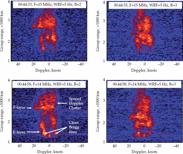
Figure 3.30 shows mini-radar displays recorded at two frequencies spaced 1 MHz apart and in two adjacent FMS beams spaced approximately 10 degrees apart. The clutter Doppler spectrum clearly varies with range and beam as the properties of the skywave propagation paths change. The ensemble of mini-radar range-Doppler maps acquired across eight FMS beams for all interrogated frequency channels enables an operator to assess the spectral characteristics of the propagation path relevant to the main OTH radar surveillance region. The ability to rank different frequency channels based on Doppler spectrum contamination using real-time site-specific mini-radar measurements greatly assists operators to optimize frequency selection in ship-detection applications.
In a multipath environment, clutter echoes backscattered from a different patches of the Earth’s surface may be received with the same group-range and cone angle. The superposition of clutter echoes received via multiple propagation paths with different Doppler shifts and spreads will effectively contribute to broadening the clutter-occupied region of Doppler space in a given range-azimuth resolution cell. Target echoes associated with a dominant propagation mode can potentially be masked by clutter returns from a different propagation mode that is Doppler shifted relative to the dominant mode. For ship detection, the vulnerability of a channel to multimode-induced spectral contamination should also be considered for frequency selection. This type of contamination can degrade detection performance even when the individual modes have small Doppler spreads.
3.3.2 Channel Occupancy and Noise
In contrast to broadcasting, communication, and a number of other services in the HF band, OTH radars are not allocated frequencies but are permitted to use broad bands of the HF spectrum on a secondary basis. Permission to radiate is granted on the condition that the radar causes no discernable interference to other users of the spectrum, and that operation on protected frequencies (e.g., emergency channels) is forbidden at all times. In other words, OTH radars operate with strict adherence to a policy of noninterference by finding clear frequency channels of appropriate bandwidth in between other users of the HF band. Channel occupancy in the HF band not only depends on the spatial and spectral distribution of HF emitters, but also on the prevailing ionospheric conditions. As all of these factors are dynamic and unpredictable, an OTH radar requires a colocated spectrum monitor to identify clear channels in real time across the system’s frequency range.
In clear frequency channels, HF background noise from external sources usually limits detection performance for fast-moving targets (e.g., aircraft). Exceptions arise when spread-Doppler clutter is present, or if the target speed and heading give rise to a low relative velocity, where clutter may limit detection performance. In remote locations, background noise is dominated by atmospheric and galactic sources, and its power spectral density changes significantly with time, location, direction, and frequency in the HF band. Knowledge of the prevailing background noise spectral density in the surveillance region directions at the receiver site is necessary for optimum OTH radar frequency selection based on the SNR criterion.
The spectral surveillance subsystem of the Jindalee FMS includes an omni-directional spectrum monitor and a directional antenna to measure the background noise spectral density. Its function is twofold: (1) to routinely evaluate HF spectrum occupancy, such that only clear channels (not in the forbidden frequency table) are identified and potentially selected for radar operation; and (2) to measure the directional HF background noise spectral density over the radar’s angular coverage, such that clear channels eligible for use can be meaningfully ranked based on the SNR performance metric. The latter is achieved by combining background-noise data and backscatter-sounder data received in the same FMS beam.
3.3.2.1 Spectrum Monitor
Despite the shift of many services to satellite, microwave, and fibre-optic links, the HF band remains densely occupied. In addition to AM radio broadcast stations and long-range point-to-point communication systems, which continue to occupy large segments of the HF spectrum, there is an increasing proliferation of HF radars that require relatively wider signal bandwidths for surveillance and remote-sensing applications. To minimize mutual interference among users of the HF band, licenses to transmit are issued on a regional basis by national and international administrators that manage frequency allocations and schedules.
As described in McNamara (1991), a frequency allocation is nominally for a bandwidth of 3 kHz, which means that there are only about 104 channels available in the HF band to satisfy all users. In addition, most systems require access to more than a single frequency channel in order to operate effectively over diurnal, seasonal, and solar-cycle variations, which further increases demands on the finite spectrum resource. Not surprisingly, all HF band channels have been allocated many times over worldwide, at times within the same country (McNamara, 1991). To use the spectrum more efficiently, it is in principle possible for certain systems to operate independently on the same allocated frequency channel by using cooperatively designed waveforms that are “non-interfering” after processing in the receiver. For example, this principle may be adopted by cooperative networks of oceanographic HF radars.
An omnidirectional antenna located at the OTH radar receiver site is used to monitor channel occupancy in the Jindalee FMS. Using an omnidirectional (whip) antenna for this purpose ensures that man-made transmissions are not missed due to being masked in beam pattern nulls. Specifically, the HF spectrum analyzer measures the interference-plus-noise power spectral density over a frequency range of 5–45 MHz at a granularity of 2 kHz, with clear frequency channel updates provided at 2- to 10-minute intervals. For evaluation of channel occupancy, the received signal power level is evaluated in all 2-kHz channels of the spectrum. These site-specific estimates are then averaged over 10 passes and an algorithm is used to classify channels as either clear or occupied. For channels that are declared to be clear, a reliability index is ascribed based on the previous history of the channel’s occupancy (Earl and Ward, 1986).
Forbidden channels are stored in a look-up table with an in-built control feature that automatically prevents them from being inadvertently selected for radar use, irrespective of whether such channels would otherwise be declared as clear. Figure 3.31 shows an example of spectrum monitor data recorded between 17 and 18 MHz during the day by the Jindalee FMS. Occupied channels are indicated along with the background noise estimate and a clear channel of 100-kHz bandwidth, as measured at the receiver site.

FIGURE 3.31 Practical example of power spectral density containing man-made transmissions and background noise in a 1-MHz band of the HF spectrum. The data was recorded during the day (12:31 LT, March 2002) by the spectrum monitor of the Jindalee FMS located in a remote region of central Australia, 23.532 degree (S) and 133.678 degree (E). The spectrum illustrates the presence of powerful narrowband transmissions originating from different users in the HF band and an unoccupied frequency channel with a bandwidth of about 100 kHz. The power spectral density within this channel is near the estimated background noise level. If this channel is declared to be clear after multiple passes of the spectrum, it would become eligible for OTH radar use provided it is not a forbidden frequency. © Commonwealth of Australia 2011.
3.3.2.2 Background Noise
While spectrum occupancy is measured using an omnidirectional antenna, the background noise spectral density is measured on eight directional FMS beams that span the OTH radar arc of coverage. The frequency channels declared to be clear by the spectrum monitor are collectively used to estimate the background noise spectral density, with averaged values computed at increments of approximately 1 MHz across the spectrum. As the receiver site is located in a remote area, the background noise spectral density estimates in clear frequency channels are mainly due to atmospheric and galactic noise, which dominate in the lower and upper regions of the HF band, respectively.
Figure 3.32a shows the diurnal variation and frequency dependence of the estimated background noise spectral density for a particular FMS beam at the Jindalee OTH radar receive site. The background noise spectral density is observed to exhibit a relatively uniform profile in frequency around the middle of the day. However, the nighttime background noise spectral density is significantly higher at lower frequencies. In this example, the nighttime background noise spectral density in the lower HF band increases by more than 20 dB compared to daytime levels.

Figure 3.32b illustrates the monthly median background noise spectral density as a function of frequency and time of day. The significant variation as a function of time and frequency arises due the absence of D-region absorption at night and the lower critical frequency of the F2-layer at night. This enables atmospheric noise below the F2-layer critical frequency to propagate effectively over very long distances at night. Skywave OTH radars are therefore confronted with higher background noise levels at night, when lower operating frequencies need to be used, compared to the daytime, when the ionosphere supports propagation at higher frequencies.
The combination of real-time BSS data and background noise measurements made in the same FMS beam enables clear frequency channels to be ranked on the basis of SNR for a given surveillance region. The optimum frequency yielding maximum SNR changes with time as well as the azimuth and range extents of the surveillance region in the OTH radar coverage. Note that the range of the surveillance region only changes the numerator of the SNR expression (i.e., signal power) as a function of frequency, whereas a change in surveillance region direction will change both the signal power and background noise power as a function of frequency.
In summary, the combination of backscatter sounder and background noise data is required to find the optimum aircraft-detection frequency for a particular surveillance region based on maximizing SNR. Whereas the ensemble of mini-radar clutter range-Doppler maps may be used to select the optimum ship-detection frequency for a particular surveillance region in terms of minimizing Doppler spectrum contamination. In either case, the key to providing automated frequency advice to OTH radar operators is the availability of real-time and site-specific measurements that are calibrated to allow SNR- and SCR-related performance metrics to be evaluated for all directions and ranges within the coverage.
3.3.3 Ionospheric Mode Structure
Backscatter sounding and the mini-radar represent efficient techniques for measuring the power level and spectral characteristics of the returned signal echoes, respectively, but neither system provides propagation-path information in a form that is directly suitable for interpreting the ionospheric mode structure. Specifically, backscatter ionograms and miniradar range-Doppler displays are poorly suited to the resolution and identification of propagation modes, such as the two-way E, F1, and F2 modes. For F-region layers in particular, this includes high- and low-angle rays and magneto-ionic splitting of each ray into ordinary and extraordinary waves. Moreover, “mixed” modes also arise over a two-way path, as described in Chapter 2.
A detailed knowledge of ionospheric mode structure is relevant to the interaction of the radar with a point target. A target located at a fixed ground range and great circle bearing can give rise to multiple echoes detected at different group-ranges and cone angles when the signal bandwidth or antenna aperture is sufficiently large to resolve the propagation delays or angles of arrival of the ionospheric modes present. A sounder capable of identifying the ionospheric modes propagating over a particular skywave circuit, and determining the virtual height(s) of the reflecting layer(s), is not only required to reliably associate radar detections with individual targets, but also to accurately convert group-range to ground-range and cone-angle to great-circle bearing (even in the case of a single propagation mode).
An oblique incidence (OI) sounder provides a direct observation of received signal energy as a function of propagation delay (group-range) and operating frequency over a one-way point-to-point circuit. The mode-structure for the oblique path may be readily interpreted from the resulting two-dimensional image known as an OI ionogram. The frequency-dependence and group-ranges of so-called “mixed-modes” that would occur for the same oblique path over a two-way circuit may be inferred from one-way measurements by convolving the ionogram with itself, i.e., by invoking the principle of reciprocity. A vertical incidence (VI) sounder is based on the same principle as an OI sounder but observes the overhead ionosphere at near vertical incidence using appropriate transmit and receive antennas separated by a small distance.
Although OI/VI ionograms can assist with frequency selection for a particular mission, the main role of the deployed OI/VI sounders is to routinely probe strategically chosen ionospheric control points within the OTH radar coverage to facilitate the generation of a real-time ionospheric model (RTIM). A site-specific RTIM in the region of interest is valuable for associating multipath tracks to individual targets as well as for coordinate registration (CR), i.e., the process of converting tracks from radar coordinates to geographic positions. This section discusses OI and VI sounders and their relationship to the RTIM. The channel scattering function (CSF), which provides delay and Doppler information for the ionospheric modes present in a single narrowband frequency channel at a time, will be described at the end of this section.
3.3.3.1 Vertical and Oblique Sounders
The Jindalee OI/VI sounder systems are based on a linear FMCW that is swept through the HF band at a rate of 100 kHz/s. In the original Jindalee FMS, the VI sounder used a delta antenna at the transmit site to direct signals vertically upward such that the antenna at the receiver site acquired the echoes returned by the ionosphere after a near-overhead reflection. For the oblique path, a remote low-power broadband transmitter feeding a bowtie antenna was used. In both cases, the received signal is downconverted, filtered, and analyzed in 610-ms time frames, which corresponds to an effective bandwidth of 61 kHz and a one-way group-range resolution of 4.9 km. OI/VI ionogram traces covering the full HF band may be updated in under 5 minutes. “Clean-up” algorithms are typically used to remove narrowband RFI in order to display the ionogram traces more clearly.
Figure 3.33 shows example OI ionograms recorded by the Jindalee FMS system for the Darwin to Alice Springs HF link (over a ground distance of approximately 1250 km) during the day and night. The variation in mode content as a function of frequency across the HF band and the change in mode content with time of day at a particular frequency is clearly evident in these examples. Inspection of the ionogram trace allows the ionospheric modes that propagate the signal at a particular frequency to be identified, as described in Chapter 2. The virtual reflection height corresponding to each ionospheric layer affording propagation may also be estimated from the power-delay profile due to the known positions of the transmit and receive sites. Automatic recognition of specific trace features enables ionospheric parameters such as the layer critical frequencies and heights to be extracted using software tools from the recorded ionograms without the need for manual interpretation.

OI sounders may be used to determine the strength and time dispersion of ionospheric modes to optimize frequency selection in long-range point-to-point HF communication systems. Link quality for certain systems can be improved by selecting carrier frequencies where skywave propagation is effectively due to a single dominant mode of adequate SNR. In Figure 3.33b, the best range of operating frequencies for almost single-mode propagation occurs between 6 and 7 MHz. Over this range of frequencies, propagation is mainly due to the low-angle ray of the F2-layer. Both magnetoionic components are present, but cannot be resolved in group delay. In OTH radar applications such as ship-detection and remote sea-state sensing, an OI sounder located near or within the surveillance region can at times help to select frequencies that reduce multimode-induced Doppler spectrum contamination.
However, the main benefit of OI/VI sounder data to OTH radar is not so much for frequency selection as it is to generate and update the RTIM. This requires a coordinated network of OI/VI sounders that routinely interrogate a strategically chosen set of ionospheric control points within the OTH radar coverage. When the end point of a desired oblique path is not accessible for deploying an OI sounder station (e.g., over the ocean), a VI sounder located at the mid-point of the desired path can be used to monitor the ionospheric control point and predict the mode content of all oblique circuits with the same midpoint.
An OI ionogram provides accurate information on ionospheric mode structure for skywave paths with terminals close to those of the measured circuit. Of particular interest is the density of the network required to establish a high-fidelity RTIM over the OTH radar coverage. This depends in part on the extent to which the mode structure identified on a particular path is relevant to adjacent paths. As the number of sounders that can be deployed is far less than the number of control points that need to be monitored for OTH radar, RTIMs often need to extrapolate experimental measurements to predict the state of the ionosphere at locations where no real data is available.
Typically, VIS data may be used to predict F2-layer behavior to within 300–400 km for a quiet mid-latitude ionosphere at a time not near the terminators. Traveling ionospheric disturbances can significantly reduce the spatial scales over which the measurements may be extrapolated with adequate accuracy. The normal E-layer and F1-layer are relatively more predictable, and quite accurate empirical formulas for both layer critical frequencies based on climatological models available. Sporadic-E is more difficult to characterize in detail, and predictions tend to break down more rapidly with distance and/or time compared to the F2-layer. As the confidence of extrapolations based on a limited number of measured data points decreases, statistically smoothed ionospheric models based on historical (synoptic) databases may be progressively blended into the RTIM.
A high-fidelity wide-area RTIM is a fundamental prerequisite for mode identification and coordinate registration in OTH radar. Inversion procedures may be applied to OI/VI sounder traces of frequency versus virtual path-length (delay) to model the variation of electron density with true height in the ionosphere. Alternatively, a multi-segment quasi-parabolic (MQP) electron density height-profile model can be fitted directly to the ionogram trace. Figure 3.34 shows a sample ionospheric model of plasma frequency against true height parameterized in terms of three physical QP layers (E, F1, and F2), smoothly joined by inverse segments to form a monotonically increasing profile (i.e., without valleys). The parameters of this model vary as the RTIM assimilates ionospheric data measured at different times and locations by the sounder network. The RTIM may also change in response to other types of inputs such as known reference points (KRPs) and ionospheric data from climatological models.

FIGURE 3.34 Example of a multi-segment quasi-parabolic (MQP) ionospheric profile model used to represent the true height variation of plasma frequency for three physical layers (E, F1, and F2). As illustrated for the F2-layer, the QP profile is defined by three physical parameters referred to as the critical frequency foF2, true height hmF2, and semi-thickness ymF2. In the MQP model, the individual layer profiles are smoothly joined by inverse segments to form a resultant electron density profile that monotonically increases with height (with the possible exception of sporadic-E). © Commonwealth of Australia 2011.
Ray-tracing techniques may be applied to the RTIM to predict signal-propagation path characteristics over very wide areas. In particular, the MQP profile permits computationally efficient analytical ray-tracing procedures to be used (Dyson and Bennett 1988), subject to the assumption of a locally spherically-symmetric electron-density height-profile and the use of a first-order approximation for magneto-ionic (o/x) ray splitting; see Bennett, Chen, and Dyson (1991), and Chen, Bennett, and Dyson (1992). Accurate propagation-path information is required for mode-linking and coordinate registration of the OTH radar tracks.
3.3.3.2 Channel Scattering Function
The channel scattering function (CSF) provides an assessment of ionospheric propagation in a narrowband frequency channel over a one-way path by measuring the distribution of received signal power as a function of path delay, Doppler-shift, and possibly angle-of-arrival if a receiver array is used. As opposed to the OI sounder, which integrates the total received power at a particular group-range over all Doppler shifts, the two-dimensional CSF spectrum measures the delay-Doppler coupling of the received power.
Figure 3.35 shows an experimental CSF spectrum recorded by a single receiver. This example illustrates the offsets and spreads of the three dominant propagation modes in the delay-Doppler plane. In other words, the CSF provides a detailed evaluation of multimode time and frequency dispersion (offsets and spreads) for a particular HF path and narrowband channel.

FIGURE 3.35 Channel scattering function recorded on a single receiver for an ionospheric path that linked sites near Longreach and Darwin, Australia, over a ground distance of approximately 1850 km (April 2003). The peak with highest amplitude and smallest delay is contributed by the low ray of the F2-layer, which contains the unresolved o- and x-waves. The other two peaks with progressively smaller amplitudes and larger delays are due to the resolved o- and x-waves in the high ray of the F2-layer, respectively. © Commonwealth of Australia 2011.
In essence, the CSF is configured as a one-way oblique-path radar using low-power transmissions and range-Doppler processing based on a repetitive linear FMCW swept over a narrow bandwidth. The purpose of the CSF is not to detect targets, but to provide a detailed assessment of the limits imposed on narrowband HF signal detection and estimation by the ionospheric propagation channel. The transmitted signal may be acquired on an array of antennas connected to a multi-channel digital receiver. This extends the CSF measurement capability to include offset and spread in angle of arrival, jointly with delay and Doppler (i.e., a three-dimensional spectrum of the received signal).
A detailed analysis of CSF data recorded on the very wide antenna aperture of the Jindalee OTH radar receiving array will be presented in the second part of this text to reveal the fine structure of skywave propagation and to model the angle-delay-Doppler characteristics of a quiet mid-latitude ionospheric channel. The CSF measured on an array is perhaps the most fundamental indicator of the characteristics of a narrowband skywave HF channel for an OTH radar using linearly polarized receive antennas.
3.4 Historical Perspective
This section provides a brief historical perspective on the evolution of skywave OTH radar systems in the United States (US) and Australia. The operational significance and major highlights of the most important OTH radar systems in the United States and Australia will be discussed separately to provide a chronological thread of national development. For brevity, OTH radar research and development outside of the United States and Australia will not be covered in detail. However, early HF radar work in the United Kingdom (UK) during World War 2 (WW2) is briefly recalled at the start of this section to provide background leading up to the emergence of OTH radar. On the other hand, future prospects for next-generation OTH radar systems are mentioned at the conclusion of this section to indicate the possible way ahead.
There are numerous other countries outside of the United States and Australia with previous or currently active HF radar programs, although only a few of these programs have led to the development of operational skywave OTH systems. For example, substantial efforts have been invested to develop skywave OTH radar systems in Russia, Ukraine, China, and France. A description of OTH radar developments and achievements in Russia and Ukraine can be found in Evstratov et al. (1994), while a detailed discussion of the French OTH radar “Nostradamus” is available in Bazin et al. (2006). General descriptions of OTH radar and ionospheric studies conducted in China appear in Zhou and Jiao (1994), Li (1998), and Guo, Ni, and Liu (2003).
3.4.1 Past and Present Systems
The development of HF radar during WW2 evolved almost exclusively for line-of-sight (LOS) surveillance applications. Much less attention was paid by comparison at the time to the possibility of target detection and tracking at OTH ranges. The Chain Home (CH) system, developed on the east coast of the United Kingdom after the success of the Daventry experiment in 1935, was an operational network of integrated HF LOS radars. The real-time air picture provided by the CH system allowed the Royal Air Force (RAF) to deploy limited fighter resources effectively at the required time and location in the Battle of Britain. This decisive capability first demonstrated the operational value of radar for air-defense during wartime.
The CH system operated with a high peak-power of 350 kW (subsequently 750 kW) at frequencies between 20 and 30 MHz. The radar signal was a simple AM-pulse of 20μs duration with a repetition frequency of 25 or 12.5 Hz. The transmitted waveform was synchronized to the frequency of the mains to provide a common time-reference such that different CH stations did not interfere with each other. The CH transmit and receive systems were separated for isolation, but the radar configuration maintained a quasi-monostatic characteristic with respect to the coverage. The broad transmit beam provided “floodlight” illumination over the entire surveillance volume, while the receive antenna array of orthogonal half-wave dipoles (stacked on wooden towers 215-ft tall) was capable of azimuth and elevation angle estimation. A detailed description of the CH system can be found in Neale (1985a).
Although the CH system was not intended to detect targets beyond the LOS, skywave signals backscattered from the Earth’s surface at OTH ranges were occasionally received. These long-range returns represented a source of nuisance or clutter for CH radar operators when they appeared. Later during WW2, technology became available to generate sufficient power for radar systems to operate at frequencies above the HF band. Using higher frequencies allowed the development of more compact and competitive radar systems for the LOS surveillance application relative to those implemented at HF. This motivated the transition to LOS surveillance radars that operated in the UHF and microwave frequency region.
The first operational bistatic radars capable of aircraft detection and localization using noncooperative transmissions were developed in Germany and installed at various sites across the English Channel during WW2 to exploit the floodlight illumination of the CH system. A technical description of the Klein Heidelberg passive radar system and the Electronic Warfare (EW) context in which it evolved is provided in Griffiths and Willis (2010). The companion paper Griffiths (2013) discusses the operational significance and performance of two other German WW2 HF radars, ELEFANT and SEE-ELEFANT. These systems were used to perform the first active bistatic radar experiments with the potential to detect and localize target echoes.
It is reported in Trenkle (1979) that an Arctic convoy of ships near Jan Mayen Island was detected using the ELEFANT radar located at Castricum, Netherlands, at a range of 2200 km, under favourable ionospheric conditions in August 1944. This report is confirmed by two other references in Griffiths (2013). It is unclear how frequently or reliably such detections could be made, or if the radar had been cued onto the targets. In any case, such a report may indicate the first ship detection by an HF radar system at OTH ranges using the skywave propagation mode.
3.4.1.1 MADRE OTH Radar
Following WW2, the Naval Research Laboratory (NRL) in the United States considered the use of HF radar with the specific intention of exploiting skywave propagation to detect targets at ranges an order of magnitude greater than was previously possible using conventional LOS radar systems. By the late 1940s, experimental investigations with this newly envisioned goal in mind were ongoing by a number of groups in several different countries (Headrick and Thomason 1998). However, a general feeling at the time was that HF radar had little use except for in the application of oblique backscatter sounding to provide a propagation-path indicator for frequency selection in long-range HF communication systems.
Due to the “look-down” geometry of the skywave propagation path, echoes backscattered from air or surface targets at OTH ranges cannot be discerned from much more powerful ground clutter returns in a single radar pulse. Besides the very large clutter-to-signal ratio, the low signal-to-noise ratio in a single radar pulse posed another major obstacle to the success of OTH radar. It was quickly recognized that OTH radar would only succeed if echoes from moving targets could be discriminated against the much stronger but “stationary” surface-clutter returns by matched-filter Doppler processing. This technique required Doppler integration of the received echo energy over a number of phase-coherent radar pulses. In principle, such processing would not only resolve the clutter issue, but also provide the valuable SNR gain needed for reliable target detection against noise.
Effective matched-filter Doppler processing required HF receivers with sufficiently high dynamic range to acquire faint target echoes and powerful clutter returns without distorting the spectral characteristics of the signals, as well as the technology to perform coherent integration of the received echoes over a processing interval. Moreover, for the Doppler processing technique to work effectively, the ionosphere must not induce significant spectral contamination on the HF radar signals reflected from one or more layers over a two-way path. For this reason, it was necessary to measure the frequency stability of the ionosphere for the propagation of narrowband HF signals over long-distance skywave paths. This represented an essential first step toward establishing the feasibility of a full-scale OTH radar in the region of interest.
In the 1950’s, an experimental system capable of storing signal samples on a magnetic drum to allow playback with time compression and Doppler processing was developed at NRL based on several emerging signal-processing technologies. This system was initially designed for frequencies in the lower VHF and upper HF bands as means to increase SNR in radar systems. It had been developed at a time of general interest decline for skywave OTH radar and was not originally intended for such application (Headrick and Thomason 1998). However, when this new technology was used to examine high-resolution Doppler spectra of ground backscatter received via skywave propagation, the Earth echo was found to be well localized in Doppler frequency despite its very large amplitude. This important finding led to a resurgence of interest in skywave OTH radar and the newly developed equipment was later put to use in that direction.
In 1956, NRL completed a definitive set of experiments confirming that the necessary prerequisites to allow aircraft detection with OTH radar could be satisfied by a full-scale system (Thomason 2003). The ionosphere was found to be sufficiently frequency stable for aircraft target detection, while the ability to perform matched-filter Doppler processing of radar echoes using “magnetic drum recording equipment” (MADRE) was successfully demonstrated in 1958. These developments attracted the sponsorship required to pursue the construction of the first skywave OTH radar at Chesapeake Bay in the United States. This radar was named MADRE, which perhaps reflects the observation made in Headrick and Skolnik (1974) that “the signal processor was the key element to the success achieved with OTH radar.”
MADRE began operations in the fall of 1961, and demonstrated its ability to detect and track aircraft targets on North Atlantic air routes at ranges an order of magnitude greater than conventional microwave radars. With further improvements to the dynamic range of the data processor, surface vessels were detected and manually tracked in 1967. A detailed and authoritative description of the MADRE system appears in Headrick and Skolnik (1974). Thomason (2003) provides an excellent historical account of OTH radar development in the United States, while the characteristics and applications of several HF radars, including the MADRE system, can be found in Headrick and Thomason (1998).
MADRE was a single-site (truly monostatic) OTH radar system that made use of the same antenna for transmission and reception. The transmitted waveform was based on a coherent train of simple AM-pulses with 100 ms duration and 25-kW average power. A high-power duplexer enabled signal transmission and echo reception through the reciprocal antenna. Figure 3.36 shows the two primary antennas of the MADRE OTH radar installed at the NRL field site in Chesapeake Bay. The large fixed antenna array is shown on the left of picture, while the smaller rotary antenna appears at the top of the tower on the right.
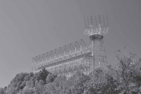
FIGURE 3.36 The two primary antennas of the MADRE OTH radar system installed on the Naval Research Laboratory (NRL) field site at Chesapeake Bay (photograph courtesy of NRL and Dr G. Frazer).
The high-gain primary antenna was a fixed (98-m-wide and 43-m-high) phased array of horizontal dipoles in corner reflectors stacked two high and ten wide. The antenna beam could be electronically steered in azimuth up to 30 degrees from boresight by adjusting the lengths of feed cables. The phasing applied to the two horizontal rows provided some degree of elevation steering. The high-gain primary antenna was used for target detection and tracking at long ranges via the skywave mode. The low-gain primary antenna consisted of two in-phase horizontal dipoles in a corner reflector mounted on a 200-ft high tower. This smaller antenna was steered by mechanical rotation and routinely used to monitor US ballistic missile launches. A vertically polarized folded triangular monopole with a back screen was used to detect targets via the surface-wave mode over the sea.
MADRE is widely recognized as the first radar system to detect and track aircraft at ranges an order of magnitude greater than conventional microwave radars. This system had modest capabilities and was not intended to represent an operational prototype for wide-area surveillance. Its historical importance lies in the success of exploiting matched-filter Doppler processing for frequency resolution and coherent gain. The MADRE OTH radar represents a ground-breaking system for demonstrating the ability to detect and track targets at ranges of thousands of kilometres via the skywave propagation mode. Indeed, this system was the first to discover most of HF OTH radar’s target detection capabilities.
3.4.1.2 Wide-Aperture Research Facility (WARF)
In the 1960s, students and technical staff at Stanford University designed and built an alternative skywave OTH radar system known as the Wide Aperture Research Facility (WARF) at two major field sites in the central valley of California. This revolutionary system was sponsored by the Defense Advanced Research Projects Agency (DARPA) and subsequently became a Standford Research Institute (SRI) International facility in 1967. Experimental measurements of the spatial coherence of skywave signals received by the WARF first showed that antenna apertures more than 2.5-km long could be used to form coherent beams with high gain and resolution for OTH radar systems (Sweeney 1970).
The WARF design philosophy departed significantly from that of the MADRE OTH radar and was paradigm-shifting in a number of respects. Besides employing completely different antenna elements and array designs on transmit and receive (described below), the WARF transmit and receive sites were separated by about 100 nautical miles. Indeed, WARF pioneered the use of linear frequency–modulated continuous waveforms (FMCW) in conjunction with the two-site OTH radar architecture known as the quasi-monostatic configuration. Use of a constant-modulus waveform with unit duty-cycle substantially improved radar sensitivity against noise (SNR), while the larger time-bandwidth product of such waveforms compared to AM-pulses of equivalent range-resolution enabled the out-of-band emissions to be suppressed more effectively, which made HF radar an acceptable occupant of the HF spectrum.
Unlike MADRE, which used the same vertical curtain array of horizontal-dipole antenna elements for transmission and reception, the WARF system employed a dual-band uniform linear array (ULA) of vertical LPDA elements matched to the lower and upper HF band. This dual-band feature combined with the inherent broadband characteristic of the LPDA element allowed WARF to operate over a wider frequency range than MADRE. The WARF receive system was based on 2.55-km long ULA consisting of 256 twin-whip end-fire receiving pair (TWERP) antenna elements spaced 10 meters apart (Barnum 1986). The receive elements were matched to the upper HF band, where the power spectral density of external noise is typically lower. The wide aperture of the WARF receiver array provided fine spatial resolution, which increased radar sensitivity against clutter (SCR) and spatially structured interference. It also improved target localization accuracy.
The relatively broad beam of the WARF transmit antenna was used to floodlight a surveillance region within the OTH radar coverage, while a number of high-resolution receive beams were electronically steered across the illuminated region to simultaneously acquire the backscattered echoes. The WARF system first demonstrated this operational concept, which permitted the instantaneous coverage of the OTH radar to be decoupled from the spatial resolution of the receive antenna. Besides providing an effective wide-area surveillance capability for aircraft targets, the WARF architecture significantly enhanced ship detection performance in a clutter-limited environment with respect to MADRE. WARF is of fundamental importance in the history of OTH radar as it represents a legacy system upon which currently operational designs in both the United States and Australia are based. A detailed description of WARF can be found in Barnum (1993).
3.4.1.3 AN/FPS-95 (Cobra Mist)
Following the success of MADRE, the AN/FPS-95 skywave OTH radar system, also known by its code-name “Cobra Mist,” was developed jointly by the US Air Force and the Royal Air Force at Orford Ness in Suffolk, England. The missions of the AN/FPS-95 included the detection and tracking of aircraft as well as the detection of missile and satellite vehicle launchings in Eastern Europe and over western areas of the former Soviet Union. Cobra Mist was also intended to provide a research and development test-bed to determine effective OTH radar techniques for other operational missions. Site works for the project began in mid-1967 and construction was completed by the contractor, Radio Corporation of America (RCA), in July 1971.
Cobra Mist was a single-site OTH radar system that used AM-pulse waveforms, similar to MADRE, but the peak power that could be generated was much greater (up to 3.5 MW). As in MADRE, the same antenna elements were used for transmission and reception. However, the Cobra Mist system was based on 18 LPDA elements or “strings” that were 2200 ft (671 m) long and contained both horizontal and vertical dipoles. The LPDA elements were oriented to form a fan shape that radiated out from a central “hub” point to provide an approximately constant beamwidth independent of frequency. The strings were separated by 7 degrees and occupied a sector of a circle that spanned an angle of 119 degrees. Six adjacent LPDA elements were combined by means of a cable switching network to form a beam. The AN/FPS-95 was the largest, most powerful, and most sophisticated OTH backscatter radar of its time. A detailed description of the system can be found in (Fowle et al. 1979).
The HF radar community as a whole had expected that Cobra Mist would set new standards in performance and capability for the OTH radar art. In practice, quite the opposite transpired. The original plan to commence operation in July of 1972 was delayed because Cobra Mist was plagued by a serious “clutter-related” noise problem of unknown origin that severely limited sub-clutter visibility to values not much greater than 60 dB. As the source of this noise could not be conclusively identified after an extensive series of site tests, the project was terminated abruptly in June 1973. The system was subsequently dismantled and the components removed from site. Malfunction of radar equipment was exonerated from being the cause of the problem, although not with complete certainty. The order of magnitude increase in transmit power with respect to MADRE, coupled with the relatively coarse spatial resolution of the AN/FPS-95 antenna, would have required receivers with high linearity and spurious-free dynamic range to avoid self-inflicted limitations in system performance.
The hypothesis that jamming caused the clutter-related noise could not be confirmed or denied by site tests. Natural phenomena producing spread-Doppler clutter in the high-latitude ionosphere could also not be excluded as the possible cause, particularly as the antenna beam pattern was not designed to suppress such signals effectively. The declassified report (Fowle et al. 1979), submitted by MITRE engineers called upon to determine why the AN/FPS-95 did not meet performance expectations, provides a detailed account of the attempts made to locate and correct the source of the noise, which remains an enigma to this day.
3.4.1.4 AN/FPS-118 (OTH-B)
In the late 1970s, the US Air Force developed a two-site OTH radar system known as the AN/FPS-118 in partnership with General Electric. The initial phase of this project was an experimental system located in Maine that served as a technology demonstrator. The AN/FPS-118 system operated in a quasi-monostatic configuration with an inter-site separation of about 160 km. This system operated using the linear FMCW technique pioneered on the WARF, but the transmit power was an order of magnitude greater. As shown in Figure 3.37, the AN/FPS-118 adopted canted-dipole antenna designs instead of the LPDA elements used in WARF. It is argued that such antennas provided robust low-elevation performance in the presence of reduced ground conductivity, particularly when snow and ice covered the area surrounding the array.

FIGURE 3.37 Canted-dipole elements used in the transmit antenna arrays of the US Air Force AN/FPS-118 (OTH-B) radar systems developed by General Electric in Maine and Oregon.
In the early 1980s, the AN/FPS-118 transitioned from an experimental program to a full-scale operational development (OTH-B) under contract with General Electric. The US Air Force OTH-B systems were installed as three-sector radars on the east and west coasts of the United States in Maine and Oregon, respectively. The primary mission of the six OTH-B systems deployed (i.e., three east and west coast radars) was to detect aircraft and cruise missiles across two 180-degree azimuth sectors spanning a one-hop coverage area of more than 30 million square kilometers over the Atlantic and Pacific oceans.
At each OTH-B site, the transmit antenna consisted of 3 contiguous 6-band linear arrays of canted-dipoles with 12 elements per band and 41-m-high backscreens. Each 6-band linear array provided 60 degree coverage in azimuth using antenna apertures of 304, 224, 167, 123, 92, 68 m for operation over a frequency range of 5–28 MHz. The three contiguous transmit arrays were oriented 60 degrees apart to provide 180 degree coverage in azimuth at ranges between 900 and 3000 km. The OTH-B radars operated with a maximum transmit power of approximately 1 MW using linear FMCW with PRFs of 10–60 Hz, bandwidths of 5–40 kHz, and CPIs of 1–20 seconds (Skolnik 2008b).
The receive antenna of the OTH-B radar was implemented as three contiguous linear arrays of 246 × 5.4-m vertical monopoles with 20-m backscreens. The receive apertures were 1519 m long and contained 82 reception channels. Each of the arrays provided 60 degree coverage in azimuth with the three boresights oriented 60 degree apart. A detailed description of OTH-B can be found in Georges and Harlan (1994). Hughes (1988) reported on a series of tests validating the capability of OTH-B to detect cruise missiles. A distinguishing feature of this system is that it was the first operational skywave OTH radar in the United States that possessed a genuine wide-area surveillance capability for continental air-defense (Headrick and Thomason 1998). In 1991, the US Air Force put the OTH-B system in “warm storage” in response to the perception of a reduced air threat (Thomason 2003).
3.4.1.5 AN/TPS-71 (ROTHR)
The design and procurement of the US Navy AN/TPS-71 system, also known as the relocatable OTH radar or “ROTHR,” was driven by the threat of long-range bombers and missile carriers to the battle group at sea (Thomason 2003). Under the sponsorship of the Chief of Naval Operations, the Space and Naval Warfare Command awarded a contract to the Raytheon Corporation in 1984 for the full-scale development phase of AN/TPS-71. The concept was that ROTHR could be air transported in containers and assembled quickly for operation at preprepared sites to counter the identified threat.
A prototype system was constructed and tested in Virginia, after which it was relocated and tested again. Based on the successful evaluation of the ROTHR system, a total of three production units were built. The first of these systems is currently installed in Virginia, the second in Texas, and the third in Puerto Rico. These current sites were selected to monitor air and surface drug-trafficking routes into the United States, which became of concern after the open-ocean air threat to the battle group diminished. Aerial photographs of the ROTHR transmit and receive sites in Virginia are shown in Figure 3.38.
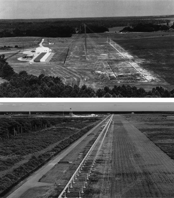
FIGURE 3.38 The top and bottom photographs show the transmit and receive sites of the US Navy AN/TPS-71 Relocatable OTH Radar (ROTHR) located at Chesapeake and New Kent, in Virginia, respectively. (Pictures courtesy of the ROTHR Program).
The ROTHR transmit system in Virginia is situated on a 20-hectare site in the Chesapeake area. The transmit antenna is a two-band linear array of 2 × 16 LPDA elements (75–125 ft or 23–38 m tall) designed to operate at frequencies between 5 and 28 MHz. The maximum average power is around 200 kW, and similar to WARF, the quasi-monostatic configuration enables ROTHR to exploit linear FMCW operation. The instrumented range of selectable PRF, bandwidth, and CPI parameters caters for both aircraft and ship detection missions. The transmit beam may be steered in azimuth over a ±30 degree arc from boresight. The ROTHR system currently provides wide-area surveillance of drug-trafficking routes into the United States at ranges of up to 2000 nautical miles (1 nautical mile is equal to 1.852 km).
The receiving aperture is a uniform linear array of 372 vertical twin-monopole antenna elements steered at endfire to provide an appropriate front-to-back (directivity) ratio. The twin-monopole antenna elements are 5.8 m tall and uniformly spaced approximately 6.95 m apart to yield a receive array with a 2580-m-long aperture. The array has a digital reception channel per element and the receive beam may be steered in azimuth to ±45 degrees from the boresight direction. A detailed description of the US Navy’s ROTHR systems, which are heavily based on the WARF design, appears in Headrick and Thomason (1996).
3.4.2 OTH Radar in Australia
Australian HF radar programs commenced in the 1950s. These included experimental investigations into skywave-path stability with an eye to OTH radar (Sinnott 1988), but the initial focus was on line-of-sight observations of RCS enhancements as rockets left and reentered the Earth’s atmosphere from a test range near Woomera, in central Australia. RCS enhancements due to ionization in the engine exhaust plume were observed, but this phenomenon was significant only after the missile had reached altitudes of about 100 km with the engine still burning. Such results received considerable interest in the United States because of their potential relevance to ballistic missile detection during the boost phase.
In addition to the scientific impact of this early research, a considerable amount of indigenous skill and experience in performing field trials had already been developed in Australia by the end of the 1960s. This expertise subsequently proved to be of considerable influence and importance in helping to form a collaborative research agreement on OTH backscatter radar between Australia and the United States in 1969. Exposure to US knowledge and technology was a key element that enabled OTH radar development to proceed in Australia.
The current JORN system was preceded by two main phases of the Jindalee project, referred to as Jindalee Stages A and B, as well as an earlier project to quantify ionospheric path stability in the Australian region, known as GEEBUNG. An excellent historical account of the evolution of HF radar in Australia between the 1950s up to the mid-1980s is provided in Sinnott (1988), while Colegrove (2000) summarizes skywave OTH radar developments in Australia from the mid-1980s to the year 2000. This section briefly overviews the various stages of OTH radar research and development in Australia culminating with the JORN system.
3.4.2.1 GEEBUNG
Although it had been revealed that skywave OTH radar had been tested in the United States and that the detection of aircraft targets at ranges of thousands of kilometers had been achieved, it was necessary to confirm that ionospheric conditions in Australia would not preclude effective OTH radar operation. The first experimental studies to ascertain the feasibility of OTH radar in the Australian region commenced in 1970 with a project known as GEEBUNG. This project utilized a frequency-modulated continuous wave transmitter and receiver, both of US design, in addition to communications equipment and antennas of local design.
This project involved a long measurement campaign to monitor the characteristics of ionospheric propagation between two stations separated by a ground distance of 1850 km. The transmit site was located at Mirikata, near Woomera, while the receive site was situated close to Broome, on the north-west coast of Australia. Over an 11-month period, one-way path-loss and Doppler stability measurements of the skywave propagation channel were made by Dr Malcolm Golley. Meanwhile, backscatter experiments to assess the properties of two-way propagation over land and sea surfaces were performed by Dr Fred Earl.
The main recommendation of the data analysis, which appeared as the last sentence of an overview report prepared at the conclusion of GEEBUNG, was that there was no evidence to suggest that the “operational value of an OTH radar in Australia would be reduced to an unacceptable level by inherent physical limitations imposed by the ionosphere.” This finding supported the proposal for a pilot radar as the next phase of the project. The GEEBUNG experimental sites were decommissioned in 1972, but the conclusions of the data analysis would be far-reaching. Indeed, the concept of a pilot radar led to the birth of the Australian OTH radar project “Jindalee.”
3.4.2.2 Jindalee Stage A
Stage A of the Jindalee project officially commenced in the beginning of 1974. It involved the development of a non-scanning OTH backscatter radar with an architecture based on the design of the WARF system. Two sites were identified in a remote region of central Australia, not far outside of Alice Springs. Specifically, the transmit site was located at Harts Range (100 km north-east of Alice Springs), while the location ultimately chosen for the receive site was at Mt Everard (40 km north-west of Alice Springs). The two sites and the radar boresight were selected to observe targets of opportunity (mainly commercial jets) on an international air route in a north-westerly direction. In particular, the fixed “staring” beam of the Stage A radar provided a limited sector of coverage (a few degrees wide) aligned with the A76 air-traffic corridor.
The Stage A transmit antenna was a ULA of 16 LPDA elements borrowed from the United States, while the receive antenna was a locally designed 640-m-long ULA consisting of 128-whip antennas arranged as doublets. The waveform generator and signal processor were also locally manufactured and represented advancements in the state-of-the-art. The latter was adapted from the Programmable Signal Processor used in the sonar program that led to the Barra system, while the former involved the development of a linear sweep generator that met extremely stringent demands on spectral purity. Establishing an OTH radar technology base in Australia was widely regarded to be an essential part of the project.
The Jindalee Stage A radar commenced operations in 1976, and after years of preparation, it was fitting that an aircraft was detected during the initial checkout phase (Sinnott 1988). Routine logging of target detections over a 2-year period and off-line analysis of recorded data demonstrated a credible aircraft detection capability. A large amount of environmental data was also recorded to guide future OTH radar development. Although not planned, or expected for the capabilities of the Stage A system, ship detection trials performed in December 1977 demonstrated that the detection of surface vessels off the northwest coast of Australia was feasible.
The approval for Stage B of Project Jindalee was conditional on the performance of Stage A. The provision was made for a “hold” period after the completion of Stages A, during which the results of the system would be critically reviewed and assessed before agreement was given for Stage B to proceed. To support the case for a Stage B radar, a live demonstration of the system’s capability was organized. A cooperative aircraft was commissioned for a special trail to be witnessed by a high-level delegation that had been invited to visit the receiver site in April 1977. The importance of the success of this trial in winning over the support of senior officers that were present on the day of the demonstration is described in Sinnott (1988).
3.4.2.3 Jindalee Stage B
Based on the success of Stage A, a second much more ambitious phase of the Jindalee project was approved in 1978. Stage B involved the development and demonstration of an OTH radar with operational capabilities. Radar sensitivity was increased by using a larger number of more powerful transmitters in addition to a much larger receive array. The Stage A transmit antenna was retained, but a major outcome of the performance-cost tradeoff study was the design of a receive array with a 2.8-km-long aperture consisting of 462 uniformly spaced dual-fan antenna elements. A 3 km by 100 m strip of land was cleared for the receiving array, and its quite remarkable that a man and his wife installed all of the 924 (single-fan) antenna elements in 32 days while camping at the receiver site (Sinnott 1988).
The requirement for track-while-scan over a sector of least 60 degrees called for much more powerful computing than was used in the Stage A system. As a processor suitable for the task was not commercially available at the time, a custom-designed processor known as the ARithmetically Oriented (ARO) processor was specifically developed for the Stage B radar. The design and implementation of this signal processor, including the programming language, software operating system, and digital hardware, was necessary to ensure that the Stage B radar could fulfill its real-time surveillance requirement without depending on the future availability of commercial off-the-shelf technology that was fit for the purpose.
To reduce system cost and processing load, the 462 antenna elements of the receive array were grouped into 32 overlapped subarrays, with each subarray steered to the direction of the transmitter footprint via analog beamforming. A reception channel per subarray architecture significantly reduced the number of receivers (which represented a significant proportion of the system cost) and eased demands on the ARO signal processor, while allowing high-resolution “finger-beams” to be processed within the surveillance region by digital beamforming (Sinnott and Haack 1983). In favorable environmental conditions, both the transmit and receive apertures could be operated independently as left and right halves in the Stage B design to improve the real-time coverage or coverage rate.
The Stage B radar was software controlled to a much greater extent than the Stage A system, which relied more so on manual configuration of the radar through switch settings and cable connections (Sinnott 1988). The rudimentary display capability of Stage A was replaced by more user-friendly interfaces in Stage B to improve system control for radar operators. The Frequency Management System was also significantly expanded in accordance with the increased radar capability. The wide arc of coverage also meant that more beacons were deployed to support Stage B operation. The Derby installation was upgraded with more capable equipment, while a main beacon site was established in the Darwin region.
Stage B ship detections were achieved for uncued targets in 1983, while automatic aircraft tracking was implemented in 1984. By mid-1984, the Jindalee Stage B radar had substantially achieved its major objective of demonstrating the capabilities required for Australian defence surveillance (Sinnott 1988). The transition from Stage A to Stage B took roughly 6 years to complete. After a series of successful service evaluation trials between 1984 and 1987, the operational system was handed over to Defence Forces and became known as the Jindalee Facility Alice Springs (JFAS). Following a number of system upgrades described in (Colegrove 2000), JFAS was officially operated and managed by the Royal Australian Air Force (RAAF) No. 1 Radar Surveillance Unit (1RSU) on 1 January 1993.
3.4.2.4 Jindalee Operational Radar Network (JORN)
A high-level review to define the way forward after Jindalee Stage B led to a decision to develop a network of new OTH radars known as the Jindalee Operational Radar Network (JORN). After this decision was announced by the Minister in 1986, the refurbishment or upgrade of JFAS assumed an important but secondary role. In the proposed plan, JFAS was also to provide a testbed for developmental purposes that would facilitate the implementation, testing, and transition of future enhancements into JORN.
It is beyond the scope of this text to recount the specific details of the transition from JFAS to JORN, but an authoritative description can be found in Colegrove (2000). For a general description of the JORN architecture and its surveillance capabilities, the reader may consult Cameron (1995). From a Defence procurement perspective, an insightful case study of the acquisition and management of JORN can be found in Markowski, Hall, and Wylie (2010). The main characteristics of the JORN radars developed by Telecom Australia, GEC-Marconi UK, and RLM USA-Australia are now briefly summarized.
The JORN OTH radar systems near Longreach (Queensland) and Laverton (Western Australia) are similar in many respects with the exception that the Laverton radar utilizes two sets of ULA apertures oriented at right angles to achieve 180-degree coverage in azimuth. Both systems operate in a quasi-monostatic configuration and employ linear FMCW signals that are modified to reduce out-of-band spectral emissions. The waveform repetition frequency, bandwidth, and CPI may vary over typical values of 4 to 60 Hz, 4 to 40 kHz, and 2 to 40 seconds, respectively, depending on whether air or ship detection tasks are being performed.
Taking the Laverton OTH radar as an example, the separation between the transmit and receive sites is approximately 80 km. The transmit antenna at Laverton is based on two adjacent 2-band ULAs of LPDA elements. The transmit array contains 14 (low-band) and 28 (high-band) LPDA elements to form apertures that are approximately 160 m long. As described in Colegrove (2000), the maximum average power is approximately 560 kW (i.e., 28 transmitters with 20-kW solid-state power amplifiers). The transmit antenna gain varies from about 20 to 30 dB over the design frequency range of 5 to 32 MHz. The transmit beam of each array may be steered in azimuth to ±45 degrees from boresight, which provides a combined coverage of 180 degrees.
To service the two transmit ULAs with orthogonal boresight directions, the JORN receive antenna at Laverton also consists of two ULA arms oriented at right angles. Each arm of the receiving aperture is 2970 m long and is comprised of 480 twin-monopole elements with an elevated-feed to improve gain at low elevation angles. A photograph of the JORN receive ULA viewed at endfire is shown in Figure 3.39. The receiver per (twin-monopole) element architecture allows fully digital beam steering over a ±45 degree arc relative to boresight. The primary mission of JORN is aircraft detection, while ship detection is the secondary mission. The Royal Australian Air Force accepted JORN into service in April 2003.

FIGURE 3.39 Each receiving antenna of the JORN Laverton OTH radar is a uniform linear array of 480 elevated-feed twin-monopole elements spaced 6.2 m apart (aperture length of 2970 m) with a reception channel per element. © Commonwealth of Australia 2011.
3.4.3 Future Prospects
The JORN may well be viewed as the culmination of more than 30 years of OTH radar research and development in Australia. However, it is also important to recognize that JORN was in many respects designed as a low-risk solution based heavily on the proven performance of the predecessor JFAS system. Moreover, the JFAS system involved significant compromises in its design. These were made to satisfy tight budget constraints in the various stages of its development. It is therefore not surprising that fundamentally new threads of research with the potential to deliver not incremental but substantial improvements in OTH radar capability would eventually emerge. This section briefly identifies some possible areas in which next-generation OTH radar systems may move beyond traditional precepts to improve performance and expand functionality.
While the LPDA antenna has many advantages as a transmitting element for OTH radar, the long array of dipoles occupies a large footprint. In addition, the radiation pattern of the LPDA element limits the coverage to about 90 degrees in azimuth. It is also the case that the resonant region of the antenna changes position significantly as a function of operating frequency. When viewed collectively, these characteristics make the LPDA element rather unsuitable for use in two-dimensional (nonlinear) array geometries. In principle, two-dimensional transmit arrays offer greater flexibility to manage the spatial distribution of illumination by allowing the transmit beam to be steered and shaped independently in azimuth and elevation. Two-dimensional arrays of omni-directional elements may also be used to provide 360-degree coverage in azimuth using a single antenna aperture.
A possible alternative to the ULA of LPDA elements is to distribute the available power across a larger number of more compact and less expensive antennas that are individually connected to transmit modules with lower power. It is well known that antenna elements comprising cages of wires or metal tubes can be used to achieve electrical shortening in height and broadband performance. A more compact transmit antenna with an omnidirectional pattern can be arranged in a two-dimensional array to enable beam steering in elevation and provide 360-degree coverage in azimuth.5 Moreover, a short rigid antenna provides greater immunity against Aeolian noise, which improves the spectral purity of radiated signals. The need for an extensive ground screen to stabilize surface impedance can also be reduced by driving the active sections against a raised counterpoise insulated from the ground at the base.
A more compact antenna is unlikely to match the broadband performance of the LPDA element, and may only perform effectively over an octave. However, an array based on a large number of such antennas with a digital waveform generator and power amplifier per element would offer the possibility to operate the transmit resource in a more flexible manner, as well as reduce the internally generated phase noise in the transmit beam by averaging independent contributions over a larger number of elements. These may be considered as additional advantages with respect to the aforementioned benefits of a two-dimensional transmit array based on more compact and rigid antenna elements. The issue of mutual coupling requires careful attention in such designs, as problems associated with this phenomenon are more complex to manage in two-dimensional arrays.
Two-dimensional transmit antenna arrays have been described for mode-selective OTH radar systems in Frazer et al. (2010), where the ability to form “non-causal” adaptive range-dependent transmit beams using an appropriately chosen set of “orthogonal” waveforms in a multiple-input multiple-output (MIMO) context is proposed to improve maritime domain awareness in disturbed (multimode) clutter conditions. Further descriptions of mode-selective OTH radars and experimental results appear in Frazer et al. (2010), Frazer, Abramovich, and Johnson (2009), and Abramovich, Frazer, and Johnson (2011).
Similar to the transmit antenna, the design of the JORN receive antenna was heavily based on the proven performance of the JFAS array (which was in turn modeled on the WARF system). The use of receive antenna elements that are appropriately matched in the operating region of the HF band combined with 2D array apertures and adaptive processing on receive has the potential to enhance target detection performance by allowing clutter and noise that exhibits significant structure in space and/or time to be mitigated more effectively than would be possible with a linear array. Furthermore, wideband direct digital receivers capable of downconverting multiple simultaneous frequency channels could potentially be incorporated in future systems such that the full aperture of the receive array may be used to perform multiple radar tasks, common aperture frequency management, coordinate registration, and other support functions, all at the same time.
It is also expected that advances in distributed computing will enable future systems to host more sophisticated adaptive signal-processing algorithms for clutter and interference mitigation, as well as allowing the performance of different signal-processing chains and trackers to be evaluated in real time such that the best output can be displayed to radar operators. At the system level, it may also be possible to further develop radar resource management approaches. Such approaches help to automatically configure radar operations based solely on mission requirements and a knowledge of the prevailing environmental conditions with minimal operator intervention. These alternative concepts have the potential to create pathways for new and exciting capabilities in future operational OTH radar systems.
____________________
1 Reciprocity of a two-way skywave propagation path not only depends on the signal passing through the same control point in the ionosphere, but also on the similarity between the elevation patterns of the transmit antenna and backscattering object.
2 FM pulses permit the duty cycle to be extended to perhaps 20 percent for air-mode PRFs.
3 OTH radar performance modeling based on environmental data is discussed in Skolnik (2008b).
4 Estimates corrupted by strong RFI are rejected, while the remaining estimates are consolidated into a single power-delay profile for each 200 kHz segment of the spectrum. See Earl (1991) for BSS RFI clean-up.
5 This class of antenna is used in the Nostradamus OTH radar described previously.
..................Content has been hidden....................
You can't read the all page of ebook, please click here login for view all page.