
As the wind speed increases beyond that necessary to fully develop the resonant waves, the first-order echoes are not predicted to increase in strength after saturation is reached at a given radio frequency. However, the second-order continuum contains contributions from the entire wave spectrum, including ocean waves of length greater than the resonant waves. Strong winds can excite and increase the spectral density of waves that are longer and faster than the resonant waves, which provide additional contributions to the second-order continuum. Typically, the power and Doppler frequency extent of the second-order clutter continuum will increase at a given radio frequency as the sea-state grows. For example, the troughs often appearing next to the Bragg lines at low sea-states may become filled by second-order clutter at higher sea-states.
The detection of very large ships with a mean (angle-averaged) RCS of 40–50 dBsm is limited primarily by the strong first-order echoes in a very confined region of the Doppler spectrum. An HFSW radar can usually detect very large ships against second-order clutter, so detection performance for this target class is only a weak function of sea-state. As a result, the detection of large vessels (typically greater than 1000 tons) is often limited by external noise at long ranges if not masked by Bragg lines. Increasing radiated power or system gain can therefore extend the detection range of such targets.
On the other hand, sea-state can strongly influence the detection of low-speed small and medium-sized surface vessels (typically less than 1000 tons) with a mean RCS of 30 dBsm, or less. The detection of such vessels is a strong function of the continuum level at the radial velocity of the target, which is determined by the radar frequency as well as the wind speed and direction relative to the radar beam. Detection of small and medium-sized (low-speed) vessels is therefore heavily influenced by wind speed and direction, as well as the choice of operating frequency.
The detection of smaller surface vessels traveling against the wind is typically possible for radial velocities greater than about 20 knots. However, the detection of small surface vessels becomes more difficult when the target moves in the same direction as the prevailing wind and when the wind blows parallel to the radar beam. In this case, detection may be possible in low sea-states (sea-state 2 or less), but becomes unlikely in high states unless the target is moving with a high radial speed in excess of 20 knots. A quantitative analysis of target blind (radial) speeds as a function of target RCS, sea-state (mean wind speed and direction), operating frequency, and CPI length can be found in Maresca and Barnum (1982). Although this analysis was conducted for skywave OTH radar systems, the general findings for the lower (nighttime) frequencies are also relevant to HFSW radars.
For a given sea-state, the power contained in the second-order clutter continuum relative to that in the Bragg lines tends to rise as the radio frequency increases beyond that at which the resonant waves have reached their equilibrium limit. In other words, the cross section per unit area of the second-order continuum tends to grow with operating frequency for a given sea-state, while that of the first-order echo is predicted to remain approximately constant with frequency in the region where the resonant waves are fully developed.
The first- and second-order scattering cross sections per unit area of the sea may therefore be reduced by using lower radio frequencies, where the sea surface appears smoother to the electromagnetic wave and the resonant waves are less likely to be fully developed. At higher frequencies, the resonant Bragg waves have smaller wavelengths and may be saturated by relatively light winds, while the Doppler spectrum of second-order continuum is typically higher in level (relative to the Bragg lines) and has a form that is more sensitive to wind speed and direction than at lower radio frequencies.
If the radar is operated at a low frequency, where the sea is not fully developed, the energy contained in the Bragg lines and second-order continuum will be significantly reduced. Under such conditions, it often possible to detect low-speed small and medium-sized vessels to significantly greater ranges than at high frequencies. An exception may apply for very small vessels if the RCS falls into the Rayleigh region at the lower frequency.
Despite lower operating frequencies often being preferred for ship detection in HFSW radar, the use of higher frequencies may under certain circumstances improve target SCR. The underlying basis for this is that a higher carrier frequency can shift the Doppler frequency of a target echo from a location near or within the Bragg lines to a region well outside of the Bragg lines. The second-order clutter level outside the Bragg lines also increases at a higher carrier frequency, but the clutter spectral density at the Doppler frequency of the target echo may be less than that competing with the echo from the same target at a lower carrier frequency.
A higher frequency also reduces the scattering patch area due to the finer angular resolution of classical beamforming. It may also improve target RCS, particularly for smaller surface vessels. The benefits of using higher frequencies for clutter-limited detection tend to be more pronounced for small surface vessels at short ranges, where the advantages of higher Doppler shift, reduced resolution cell size, and potentially higher RCS may outweigh the increase in cross section per unit area of the second-order clutter integrated over all Doppler frequencies. This assumes that detection at the target range remains limited by second-order clutter despite the additional surface-wave attenuation at higher frequencies.
In a clutter-limited environment, it is well known that the detection of radar echoes from point targets can be improved by reducing the size of the spatial resolution cell. Unfortunately, the signal bandwidth cannot be increased beyond a few tens of kilohertz due to heavy user congestion in the lower HF band. In addition, it may be not be feasible or convenient to increase the aperture of the receive antenna beyond a maximum length of a few hundred meters, either because of economic or operational reasons, including site constraints due to land topography in coastline regions. Such factors limit the ability to reduce the spatial resolution cell area of an HFSW radar beyond a certain size.
Provided the target echo Doppler shift does not coincide with that of a Bragg line, it may be possible to improve the target SCR by increasing the CPI. Second-order clutter is a finite-bandwidth signal with relatively shorter temporal coherence than a target echo, assuming the target moves with a nearly constant velocity over the CPI. Longer integration times can therefore reduce the second-order clutter energy competing with a perfectly coherent target echo in a particular Doppler frequency bin by narrowing the analysis bandwidth.
The benefit of using longer CPIs for target detection against sea clutter is not only predicted in Maresca and Barnum (1982), but has also been observed in practice (Menelle, Auffray, and Jangal 2008). To address the issue of optimizing the CPI for different types of targets, the received pulse-trains can be partitioned within the signal processing system and processed using a number of different CPI. However, the radar CPI is often optimized according to the class of target to be detected, and other issues such as range-migration and maneuvering targets (which results in Doppler spread), so it cannot be increased indefinitely without incurring penalties in detection and tracking performance. Consequently, the option of using longer CPIs is also restricted. Attempts to enhance SCR by increasing the CPI eventually become counterproductive when overall system performance is considered.
As mentioned previously, the second-order clutter power relative to that in the Bragg lines tends to increase with sea-state at a given radio frequency. An experimental study of the relationship between average wave height (an indicator of sea-state) and mean second-order clutter power between the Bragg lines was conducted in Leong (2002) at a radio frequency of 3.1 MHz. An approximate linear relationship was found when both quantities were expressed on a decibels scale. Specifically, doubling of the average wave-height increased the mean power of the second-order clutter between the Bragg lines by about 13 dB. This provides an approximate guide for scaling target detection performance against second-order clutter on the basis of sea-state.
The effect of sea-state on the detection of large and small vessels competing against second-order ocean clutter was investigated by Leong and Ponsford (2008) using frequencies of 3.1 and 4.1 MHz. Two classes of ships were considered, large cargo freighters with gross registered tonnage (GRT) in the order of several tens of thousands of tons, and smaller vessels with a GRT of about 1000 tons. The difference in angle-averaged RCS for these two types of targets was estimated to be approximately 10 dBsm. It was concluded that very large vessels could be detected against the second-order continuum regardless of sea-state due to their high RCS (in the order of 40 dBsm). The detection of large vessels may be precluded by Bragg line masking at any range (Leong, Helleur, and Rey 2002) or the low signal-to-noise ratio at ranges beyond about 150 km at night.
Second-order sea clutter was found to have a significant impact on the detection of smaller vessels, but at high sea-states only. It was concluded that small ships were difficult to detect in very rough seas with significant wave heights between 5.5 and 6.5 m beyond ranges of about 100 km. The same targets also could also not be detected in rough seas with significant wave heights between 3.6 and 4.2 m at ranges beyond about 150 km. The effective clutter RCS increases with range due to the greater cross-range dimension of the resolution cell, while the RCS of a point target with constant aspect and speed clearly remains the same. Sea clutter scattered by rough to very rough seas can therefore strongly impact the detection of small ships at longer ranges where its level is above the noise.
The results in Leong and Ponsford (2008) show that the radar tends to perform better at the lower frequency of 3.1 MHz compared to 4.1 MHz for the detection of the considered targets against sea clutter. In practice, the optimum choice of operating frequency in a sea clutter–limited environment not only depends on the ocean directional wave-height spectrum, but also on the target parameters, including RCS behavior, radial velocity, range, and azimuth relative to the mean wind direction. The signal frequency represents the main parameter that the radar can control to optimize the detection of smaller surface vessels against second-order clutter. However, for a realistic ocean directional wave-height spectrum, no single frequency can maximize the statistically expected SDR for all target locations and radial speeds.
5.3.2 Ionospheric Clutter
Although HFSW radars do not rely on skywave propagation to operate beyond the line of sight, it is obviously not possible to simply “turn off” the ionosphere for such systems in practice. Unfortunately, not all of the radio wave energy emitted by an HFSW radar is coupled to the surface-wave mode. Part of the radiated signal inevitably propagates upward and impinges on the ionosphere. Under certain conditions, some of the incident skywave energy will be reflected or scattered by the ionosphere and returned to the receiver. Reflections from the ionosphere represent a source of disturbance to an HFSW radar. Unwanted echoes received by an HFSW radar via the ionosphere are collectively referred to as ionospheric clutter.
Ionospheric clutter is detrimental to HFSW radar because it has the potential to mask target echoes at operational ranges from about 90 km up to the EEZ limit and beyond. When scattering in the ionosphere occurs from dynamic electron density irregularities, the returned echoes may be significantly spread in Doppler and contaminate the entire velocity search space. Ionospheric clutter that is spread in range and Doppler can seriously impair the target detection performance or remote sensing capabilities of an HFSW radar.
Ionospheric clutter is considered by many practitioners as one the greatest impediments to achieving consistent HFSW radar performance at ranges beyond about 90 km. For this reason, significant attention has been paid to understanding the properties of ionospheric clutter and developing techniques to reduce its impact on operational systems. This section discusses ionospheric clutter path types, range-Doppler characteristics, frequency dependence, and spatio-polarimetric properties to motivate a number of mitigation approaches.
5.3.2.1 Path Typologies
Ionospheric clutter may arise as a result of the radar signal being propagated in several different ways. An investigation into the most effective ionospheric clutter paths (i.e., those with the greatest potential to cause disturbance in an HFSW radar) was conducted by Sevgi, Ponsford, and Chan (2001) using the ICEPAC simulation software package. Three primary self-interference path categories may be identified. The first corresponds to a direct skywave path, where the transmitted signal is reflected by one or more layers in the ionosphere toward the receiver from a virtual height that may range from 90 to 400+ km, i.e., the one-way transmitter-ionosphere-receiver skywave path.
This type of path is associated with ionospheric reflections at elevation angles near vertical incidence (NVI) for a single-site HFSW radar that operates below the maximum critical frequency of the ionosphere. Clearly, bistatic HFSW radar systems with a relatively small inter-site separation are also subject to the reception of ionospheric clutter via the NVI path below the maximum useable frequency of the oblique circuit. In practice, direct backscatter from the ionosphere can at times be received from directions different to that of “specular” reflection. In a single-site system, for example, ionospheric clutter may be received from directions other than the NVI path due to large-scale ionization gradients and electron density irregularities, as well as transient echoes backscattered from meteor trails in the upper atmosphere.
The second type of signal path corresponds to two-way skywave propagation involving intermediate scattering from the Earth’s surface. In this case, ionospheric clutter may be received at lower elevation angles due to the signal being backscattered by land or sea surfaces at potentially long distances from the radar. An example of the Earth surface backscatter (ESB) path is transmitter-ionosphere-sea-ionosphere-receiver. Operation above the maximum layer critical frequency can help to mitigate radar echoes returned via the direct NVI path, but it will not necessarily eliminate ionospheric clutter received over oblique ESB paths from longer ranges due to surface scatterers that are beyond the edge of the skip-zone.
The third so-called “mixed-path” category arises due to a combination of skywave and surface-wave propagation between transmitter and receiver. This is not to be confused with mixed-path surface-wave propagation over segments of land and sea, which was discussed previously. The simplest examples in this third category include the signal path: transmitter-ionosphere-sea-receiver, with the final leg being via the surface-wave mode, and vice-versa, i.e., the transmitter-sea-ionosphere-receiver path, with the first leg being via the surface-wave mode. The former of these examples has the potential to be particularly insidious as the received disturbance has the same polarization as the target echo and also arrives at near-grazing elevation angle.
5.3.2.2 Range Occupancy
During the day, radar echoes from the normal E-layer or sporadic-E, as well from the upper D-region or mesosphere, may potentially affect HFSW radar performance at operational ranges between about 90 and 130 km. This range band applies for a single-site system when ionospheric clutter is received from the D- and E-regions by virtue of the direct NVI path. Radar resolution cells at longer ranges may be corrupted by ionospheric clutter propagated via ESB paths. Although D-region ionization and the normal E-layer effectively disappear after sunset, sporadic-E may be present at various times throughout the day or night.
Ionization levels that are sufficiently high to reflect signals in the lower HF band are always present in the F-region. Ionospheric clutter received from the F-region may contaminate longer ranges in the interval between about 200 and 400 km or greater via the NVI and mixed-paths. Ionospheric clutter received from the F-region via ESB paths will be at ranges outside of the operational HFSW radar coverage, but such returns can potentially mask target echoes when they are folded in through range-ambiguities.
In any given radar dwell, ionospheric clutter may not occupy the entire range extents quoted in the previous paragraphs for the E- and F-regions and the NVI path. For example, ionospheric clutter from a relatively thin sporadic-E layer may only contaminate a 10–15 km range band contained within the 90–130-km interval. In addition, not all ionospheric regions may simultaneously contribute ionospheric clutter as the disturbance type that limits detection performance at a particular operating frequency. For example, mainly E-region returns will be received during the day when operation is below the E-layer critical frequency, despite the presence of F-region layers above it.
In addition, the range occupancy of ionospheric clutter varies over time, particularly when returned from the F-region. Figure 5.25 shows the variation in nighttime F-region ionospheric clutter power received as a function of range by a single-site HFSW radar on the east coast of Canada. Note that the range at which the nearest (NVI) echoes are received varies from below 250 to about 400 km in about 5 hours between 00:00 and 05:00 UT. Ionospheric clutter possibly returned via mixed-paths is also evident in the display.

In unfavorable conditions, the range occupancy of ionospheric clutter can be broad and potentially contaminate the entire coverage from 90 km up to the 200 nautical mile EEZ limit (370 km). In particular, ESB and mixed-path propagation described previously can significantly increase the range occupancy of ionospheric clutter beyond that of the NVI path. It is also important to distinguish between range-coincident and range-ambiguous ionospheric clutter. The former is received from group-ranges or virtual paths lengths less than the first range ambiguity of the (periodic) radar waveform, while the latter can fold into the radar coverage from much longer range due to first- and higher order range ambiguities. The latter is also known as “range-wrapped” or “range-aliased” clutter. In the following, attention is mainly restricted to range-coincident ionospheric clutter received via the NVI path.
5.3.2.3 Doppler Characteristics
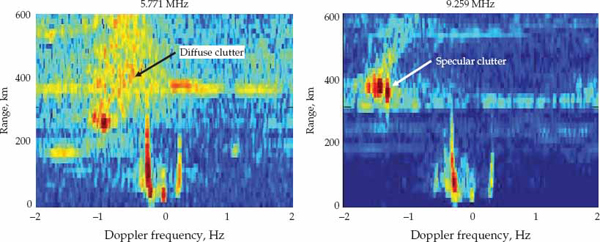
Experimental investigations confirm that the Doppler characteristics of ionospheric clutter can vary markedly in both frequency spread and centroid. The Doppler spectrum profile of ionospheric clutter may be qualitatively classified as being due to either specular reflection or diffuse scattering. The former corresponds to reflection of the radar signal from a frequency-stable ionospheric layer, which may impose a Doppler shift on the echo, but very small Doppler spread compared to the waveform PRF. In this case, the received signal is almost discrete in Doppler frequency with similar spectral characteristics to a target echo. Although specular returns can be very powerful, most of the energy is concentrated in a very narrow band of Doppler frequencies after coherent integration. These ionospheric clutter echoes are often not a problem as far as target masking is concerned, but they may cause false alarms in surveillance systems, or confuse the interpretation of the sea echo spectrum in remote sensing applications.
On the other hand, diffuse ionospheric clutter may occupy a broad band of Doppler frequencies that may approach or exceed the waveform PRF when the radar signal is scattered from dynamic electron density irregularities in the ionosphere. Contamination by so-called “fast” spread-Doppler clutter can at times mask aircraft target echoes with radial speeds of perhaps 100–200 m/s. The presence of diffuse ionospheric clutter can significantly increase the potential for target echo obscuration in the affected ranges. Figure 5.26 illustrates these two forms of ionospheric clutter, both of which are received as time-continuous signals that persist over the entire CPI. Clutter that is spread in Doppler due to the short duration of the echo relative to the CPI (e.g., transient meteor echoes) was discussed in Chapter 4.
Various physical mechanisms responsible for producing diffuse ionospheric clutter may be identified based on a combination of experimental analysis and simulations. One class of spread Doppler clutter is thought to arise due to scattering from dynamic small-scale geomagnetic field-aligned electron density irregularities produced by Kelvin-Helmholtz instabilities (Abramovich et al. 2004). Spread Doppler clutter may also arise due to large-scale atmospheric gravity waves or traveling ionospheric disturbances, which temporally modulate the signal phase-path. Another possible spread Doppler clutter mechanism is the interference of unresolved ionospheric propagation modes including “micro-multipath” rays scattered from a layer that has a spherically inhomogeneous electron density distribution.
The physical mechanisms responsible for diffuse ionospheric clutter in the E- and F-regions of the equatorial, auroral, and mid-latitude ionosphere differ significantly, but tend to be more prevalent during high sunspot years of the solar cycle when flare activity and hence the potential for geomagnetic storms is greatest. Although E-region echoes are typically more frequency-stable than F-region echoes, diffuse ionospheric clutter with significant spread in Doppler frequency may also be received from electron density irregularities in the normal E and sporadic-E layers (Thayaparan and MacDougall 2005). The reader may consult Davies (1990) for an in-depth review of the physical mechanisms responsible for spread Doppler clutter in different height regions of the ionosphere, as well as their synoptic dependence on time-of-day, season, year in the solar cycle (solar activity), and magnetic latitude.
In practice, an HFSW radar may receive a mixture of specular and diffuse ionospheric clutter. Note that purely specular (i.e., perfectly coherent) ionospheric clutter does not exist in practice, strictly speaking. In good (frequency-stable) ionospheric conditions, Doppler spread clutter components caused by imperfect temporal coherence may be received several tens of decibels below the strength of the main specular reflection peak in the Doppler spectrum. However, due to the extremely high compression gain of HFSW radar systems, which may use coherent integration times in the hundreds of seconds for slow-moving target detection, such components can still be high enough above the noise floor to limit detection performance.
As stated in (Abramovich et al. 2004), many existing ionospheric sounders cannot capture ionospheric properties over such a wide dynamic range. Current ionospheric models incorporated into software packages such as ICEPAC also find it challenging to accurately portray the characteristics of ionospheric clutter over dynamic ranges commensurate with those of modern HFSW radar systems.
Experimentally validated models capable of representing ionospheric clutter to the fine level of detail required in surveillance applications are unfortunately not available at present. This is particularly the case for systems that receive clutter from tropical or arctic regions of the ionosphere, where the physical mechanisms responsible for generating Doppler spread echoes are more prevalent (and complex) than at mid-latitudes. Such models would be of significant value to guide mitigation techniques based on adaptive processing.
5.3.2.4 Frequency Dependence
The reception of ionospheric clutter and its range-Doppler characteristics depend strongly on the choice of operating frequency. During the day, ionization in the E- and F-regions can potentially give rise to ionospheric clutter, while ionization in the D-region is mainly responsible for attenuation of skywave signals. Ionospheric clutter from the E- and F-regions can only be received via (at least) two passages through the D-layer in the day. At operating frequencies lower than the D-layer critical frequency, skywave propagation is effectively not supported due to high absorption in the D-region. Operating frequencies lower than about 3 MHz tend to be highly attenuated around the middle of the day. Operation below the D-layer critical frequency, or at frequencies near the low end of the HF band, can therefore greatly reduce ionospheric clutter received from the E- or F-regions during daylight hours.
At night, when the D-layer disappears due to electron-ion recombination, an HFSW radar may be operated above the maximum critical frequency of the ionosphere at the expense of greater surface-wave path-loss. This frequency typically corresponds to the F2-layer critical frequency, although sporadic-E can at times be the most dense layer. In principle, radio waves with frequencies above the maximum layer critical frequency will penetrate through the ionosphere at vertical incidence. In practice, ionospheric clutter may be received on NVI paths even when operating above the nominal F2-layer critical frequency due to the presence of electron density irregularities (Abramovich et al. 2004).
Moreover, oblique reflection may generate ionospheric clutter via ESB and mixed paths at frequencies above the nominal F2-layer critical frequency. The operating frequency may be raised above the maximum useable frequency (MUF) for oblique paths up to certain range. This creates a skip-zone around the transmitter, such that no backscatter can be received from the Earth’s surface within the skip-zone by the regular process of ionospheric reflection. Unfortunately, this often requires using frequencies that are too high to support effective surface-wave propagation at long distances up to the EEZ limit.
During the day, it may be possible to choose a frequency that selectively minimizes the reception of ionospheric clutter from either the E- or F-regions, but not from both layers simultaneously. For example, an operating frequency close to but not higher than the E-layer critical frequency will mainly produce E-region echoes, since the incident signals are reflected from the E-layer and do not reach the higher-altitude F-region. On the other hand, a signal frequency higher than the E-layer critical frequency (but not above the F2-layer critical frequency) will effectively penetrate through the E-region and reflect from F-region layers only.
Ionospheric clutter is typically a greater problem at night due to the disappearance of the absorptive D-layer and reflective E-layer, which may be exploited as a screen to reduce contamination from the F-region during the day. With the possible exception of sporadic-E, only the F2-layer is present at night, and the nighttime F2-layer is prone to generating diffuse (i.e., spread-Doppler) ionospheric clutter.
The range occupancy and Doppler spectrum characteristics of F2-layer ionospheric clutter may vary significantly with operating frequency. A comparison of F2-layer ionospheric clutter Doppler spectra received by an HFSW radar in the same range-azimuth cell at two well-spaced carrier frequencies is illustrated in Figure 5.27. Alternative methods to frequency selection for combating the ionospheric clutter problem, including antenna design, adaptive processing, and multi-frequency operation, are clearly needed and will be discussed later in this chapter.

FIGURE 5.27 Doppler spectra showing examples of diffuse and specular ionospheric clutter at a group range of 360 km (dashed lines). Doppler spectra at a range of 90 km containing mainly sea surface clutter with essentially no ionospheric clutter contamination are shown for comparison (solid lines). The data are from the range-Doppler display in Figure 5.26. © Commonwealth of Australia 2011.
5.3.2.5 Spatial and Polarimetric Properties
When NVI skywave returns are considered to be the dominant source of ionospheric clutter, the use of transmit and receive antenna elements with a deep and broad null at high elevation angles represents a primary mitigation strategy. However, the design of the antenna element alone is unlikely to completely remove all vestiges of NVI ionospheric clutter. Adaptive beamforming provides additional scope to discriminate between ionospheric clutter and target echoes based on differences in signal direction of arrival (DOA) or wavefront structure. Provided the ionospheric clutter has a spatial covariance matrix of relatively low rank, and the disturbance does not enter through the main lobe of the antenna beam pattern, considerable potential exists for improving the signal-to-clutter ratio by adaptive beamforming.
It has been argued that antenna arrays with elements deployed in two dimensions on the ground (e.g., L- or T-shaped arrays), provide enhanced vertical selectivity at high elevation angles to better cancel ionospheric clutter received via NVI paths. However, such array geometries may not be compatible with site constraints in coastline regions. Moreover, if there is a significant component of ionospheric clutter arriving at the receiver via the surface wave mode at near-grazing angle (due to mixed-path propagation), the added cost and complexity of a two-dimensional receive array design may not deliver the expected performance benefits. MIMO radar techniques that exploit 2D (nonlinear) arrays on receive and transmit along with a carefully chosen set of “orthogonal” waveforms may provide a form of remedy for the ionospheric clutter problem. Such systems have been discussed by Frazer, Abramovich, and Johnson (2007) in the context of skywave OTH radar.
Experimental analysis of ionospheric clutter has revealed that its spatial properties are extremely variable from one case to another (Xianrong, Feng, and Hengyu 2006a). At times, specular or diffuse ionospheric clutter returns are well localized in DOA, while at other times, the disturbance is broadly spread in azimuth (cone angle for a ULA) regardless of its Doppler spectrum characteristics. A commonly observed characteristic is that the spatial properties of ionospheric clutter are heterogeneous in time-delay and therefore need to be estimated on a range-by-range basis. Moreover, in a single range cell, the spatial properties of ionospheric clutter may additionally vary with pulse number or Doppler frequency. These characteristics significantly complicate the implementation of effective adaptive processing techniques for ionospheric clutter mitigation, particularly in terms of identifying sufficient and suitable training data.
The polarization of the received ionospheric clutter signal depends on the propagation path. Echoes received via NVI and ESB paths may be expected to be elliptically polarized, in general, as such paths involve skywave propagation directly to the receiver. On the other hand, mixed-path ionospheric clutter received via the surface-wave propagation mode in the final leg will be vertically polarized. In situations where the dominant ionospheric clutter contribution is elliptically polarized, an auxiliary set of horizontal antenna elements may provide further scope to improve SCR by means of adaptive spatio-polarization filtering.
In principle, such filtering enables the mitigation of elliptically polarized ionosphere clutter that enters through the main lobe of the receive beam pattern, where the latter is formed by using the vertically polarized antennas in the array. In practice, effective suppression of ionospheric clutter in the polarization domain requires very high correlation between the horizontal and vertical polarization components of the disturbance signal. If this correlation is not sufficiently high, or if the surface-wave contribution of ionospheric clutter on the mixed-path is significant, the potential to exploit the polarimetric properties of ionospheric clutter for mitigation is diminished.
In Abramovich et al. (2004), auxiliary horizontal loop antennas were used in conjunction with a ULA of 32 twin-monopole (doublet) elements to test this mitigation strategy. Ideally, the loop antennas do not pick up the pure ground wave signals. In practice, mutual coupling and other imperfections-limited surface-wave isolation in the loop antennas to several tens of decibels relative to the doublets. As stated in (Abramovich, Anderson, Gorokhov, and Spencer, 2004), experimental trials demonstrate that inter-polarization correlation for Doppler spread ionospheric clutter is unfortunately too low to provide any substantial mitigation capability. However, the intra-polarization spatial correlation properties were found to be quite high for both vertical and horizontal polarization components, which motivates the use of adaptive beamforming for sidelobe ionospheric clutter suppression.
5.3.3 Interference and Noise
The power spectral density of the external noise in the radar bandwidth ultimately places an upper limit on the maximum detection range of large vessels as well as smaller (air and surface) targets with radial speeds above approximately 20 knots. The main components of background noise were identified in Chapter 4, i.e., irreducible galactic noise, thunderstorm spherics, and man-made noise from unintentional radiators. In the lower HF band, atmospheric noise dominates at night in rural/remote locations and is higher in level near the equator than at the poles. Depending on the site location, incidental man-made noise may be limiting during the day in the lower HF band.
HFSW radar operation near the lower end of the HF spectrum (3–7 MHz) is often required in practice to reduce path-loss for the surface-wave propagation mode, particularly for the detection of ships at long ranges in excess of 200 km. A potential drawback of operating an HFSW radar in this frequency region is that user-congestion and the background noise level are typically greater than at higher frequencies. The reports (CCIR 1964, 1983, and 1988) and (CCIR 1970) provide HF noise spectral density estimates as a function of receiver location for different times of the day and seasons, taking into account the contribution of man-made sources separately. Operation in the lower HF band is particularly challenging at night due to the increased user-congestion and higher background-noise spectral density compared to daytime.
The significant diurnal dependence of clear channel availability and noise spectral density in the lower HF band is strongly linked to changes in ionospheric propagation conditions. During daylight hours, multi-hop skywave paths between 3 and 7 MHz are very lossy due to D-layer absorption. At such frequencies, HF interference and noise from long-distance sources are therefore highly attenuated over multi-hop paths during the day. In addition, many HF services that rely on the skywave mode tend to operate at higher frequencies during the day to exploit the increased ionospheric propagation support. The combination of very lossy long-range (multi-hop) skywave paths at low frequencies during the day, and the migration of many users to higher frequencies at this time, has the effect of reducing channel occupancy and external noise spectral density in the lower HF band compared to nighttime levels.
The D-layer effectively disappears at night and this typically allows HF signals in the 3–7 MHz band to propagate over long distances with reduced attenuation. Moreover, many HF systems are forced to move to lower frequencies at night due to the diminished support for skywave propagation at higher frequencies. In other words, the reduced ionization density in the nighttime F-region causes many users to crowd into the lower HF band, where operation via the skywave mode remains possible.
The combination of these factors results in a much greater number of interference and noise sources becoming “visible” to an HFSW radar at night. The higher user-congestion in the lower HF band at night can make it very difficult to find a clear channel on which to operate the radar, while the higher external noise spectral density can limit the detection of both fast- and slow-moving targets at relatively shorter ranges. The difference between day and night external noise spectral density levels at a fixed frequency in the lower HF band may be up to 20 dB or more.
Figure 5.28 shows the noise figure variation in 4-hour time blocks with season at a frequency of 4.1 MHz for an electrically quiet site on the east coast of Canada based on data from the final report of (CCIR 1964, 1983, and 1988). The maximum noise levels are observed to occur between the hours of 20:00 and 04:00 local time (i.e., columns 3 and 4 on the bar chart). The minimum noise levels are observed to occur between the hours of 08:00 and 16:00 local time (i.e., columns 1 and 6).
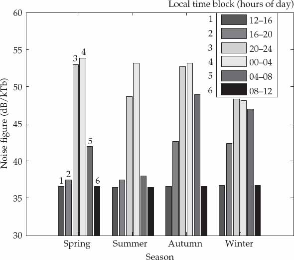
FIGURE 5.28 Noise figure at 4 MHz for a quiet site on the east coast of Canada. © Crown 2010. Government of Canada. (Courtesy of Dr. H. Leong, Defence R & D Canada.)
When D-layer absorption disappears shortly after sunset, the nighttime external noise level rises by about 15 dB with respect to the daytime level. As much of this noise is unstructured in space and time, its level cannot be reduced significantly by signal processing. HFSW radar performance therefore degrades at night. This is not only due to the degradation in SNR at all ranges, but also because ionospheric clutter from the F-region at longer ranges tends to be diffuse and is more difficult to mitigate for the reasons mentioned previously.
Incidental interference that overlaps the radar bandwidth from other users of the HF spectrum is often highly directional and sometimes structured in time. A variety of signal processing techniques that may operate in the temporal, spatial, and polarization domains (separately or jointly) have been developed to mitigate incidental man-made interference. For example, short-lived interference from transmitters such as frequency-swept ionospheric sounders may be canceled using time-domain processing techniques similar to those used for suppressing atmospheric noise (lightning discharges) provided the impulse or burst duration is short compared to the CPI, as described in Chapter 4. The theoretical and practical performance of several such methods has been analyzed and compared using experimental HFSW radar data in Lu et al. 2010.
For time-continuous or long-lived interference on the time scale of the HFSW radar CPI, adaptive beamforming represents an alternative approach for rejecting persistent signals that overlap the radar bandwidth, but are not incident from directions in the main lobe of receive beam pattern (i.e., sidelobe interference). When such interference propagates to an HFSW radar via the skywave mode, the spatial non-stationarity of the disturbance signals over the relatively long CPI needs to be taken into account for effective mitigation. A robust adaptive beamforming technique suitable for practical implementation in modern HSWR radar systems was developed and experimentally tested in Fabrizio, Gershman, and Turley (2004).
Narrowband interference has been effectively canceled using a mismatched signal processing method in Ponsford, Dizaji, and McKerracher (2005). In this procedure, orthogonal phase codes are used to create a matched channel that is sensitive to radar echoes, external interference and noise, and a mismatched channel that is only sensitive to external interference and noise. The outputs of the two channels are cross-correlated to estimate the interference and noise in the matched channel. The narrowband interference is then removed by subtracting this estimate from the matched channel. Results for this technique have been reported in Ponsford, Dizaji, and McKerracher (2003).
Skywave interference will in general exhibit an elliptical polarization state that varies in space and time due to Faraday rotation. However, the surface-wave mode can only propagate HF signals with vertical polarization effectively over the sea. By incorporating auxiliary horizontally polarized receive antennas in addition to the vertically polarized main antennas, an HFSW radar can in principle employ adaptive spatio-polarimetric filtering to cancel skywave interference entering through the main lobe of the receive beam (formed using the vertically polarized antennas). In theory, this technique provides a means to reject skywave interference received from a similar direction to target echoes (i.e., within the main beam). This potential capability represents a distinguishing feature between surface-wave and skywave OTH radar systems to be discussed further in the next section.
5.4 Practical Implementation
The practical implementation of an HFSW radar system is driven by a number of factors that influence the choice of radar configuration, the selection of radar site(s), the antenna element and array designs, as well as the receive and transmit subsystem architectures. The latter includes radar waveforms and signal/data processing techniques, which are of paramount importance to the success of an operational HFSW radar system. In view of the preceding discussion on skywave OTH radar, this section focuses on practical implementation aspects that are specifically relevant to HFSW radar. The first part of this section is concerned with HFSW radar configuration and site selection, the second considers the transmit and receive subsystems, while the third discusses signal and data processing.
5.4.1 Configuration and Siting
Radar configuration refers to the relative positions of the transmitter and receiver. For example, in a monostatic configuration, the transmitter and receiver are located at a single site, while in a bistatic configuration, the transmitter and receiver are located at two well-separated sites. A multi-static HFSW radar, wherein a single transmitter services multiple receivers, may also be considered to improve track accuracy, but such configurations will not be considered here. The first part of this section briefly reviews the benefits and shortcomings of monostatic and bistatic architectures for HFSW radar, noting that systems designed primarily for surveillance within the EEZ have been implemented in both configurations. The second part of this section discusses the selection and preparation of sites for (land-based) HFSW radar systems, as both of these aspects are prerequisites for effective operation.
5.4.1.1 Radar Configuration
In the context of HFSW radar, a monostatic configuration often does not imply the use of a reciprocal antenna for receive and transmit.3 Rather, this term often refers to the use of a single-site, which typically incorporates physically distinct but effectively colocated transmit and receive systems. A significant advantage of the monostatic HFSW radar configuration relative to bistatic systems is the expanded set of geographical coverage options. The field of view of a bistatic system is nominally limited by the overlap of the angular coverage of the transmit and receive antenna patterns. As these radiation patterns have a confined beamwidth in azimuth, the area/volume of overlap clearly maximizes for a monostatic configuration. Moreover, monostatic configurations typically lead to operational systems that are more economical to field, simpler to maintain, and easier to deploy at short notice. In addition, coastal real estate is only required at one site.
Despite these undeniable advantages, two-site systems have been preferred in several cases. A bistatic configuration permits operation using continuous waveforms, which provides higher average power than the pulse waveforms used in monostatic systems (for a given transmit peak-power rating). The inter-site separation required for bistatic systems depends on several factors, including the dynamic range of the receiver, the radiated signal power, the conductivity of the ground along the direct-wave path, and the transmit/receive antenna patterns in the direction linking the two sites. Ideally, the direct path is mainly over dry land of low conductivity in a direction well outside the azimuth sector of the radar coverage as viewed from the receiver. In practice, distances that provide sufficient isolation between the HFSW radar transmitter and receiver may vary between 40 and 100 km. Synchronization between two distant sites is usually achieved via a GPS time reference.
In principle, the transmitter and receiver do not need to be well separated when pulse waveforms are used in a single-site system. However, it has been found that separations of tens to hundreds of meters may be necessary to prevent so-called “dark noise” generated by the transmitter in the off-state from entering the receiver during echo reception. Perhaps counter-intuitively, this requirement can at times mean that the coastal length and surface area needed to accommodate a single-site system may actually exceed the combined costal lengths and surface areas of two separate radar sites in a bistatic configuration. A comparative analysis of monostatic and bistatic HFSW radar configurations, which considers waveform characteristics, coverage area, detection performance, and site selection, is reported in Marrone and Edwards (2008).
In contrast to a monostatic system, radar echoes from targets and the sea surface are not received via backscatter in a bistatic system, but rather by a process of side-scatter. The measured group-range of a side-scattered radar echo from a (point) surface-target in the surveillance region is the sum of the path-lengths from transmitter-to-target and target-to-receiver. The measured group-range of the echo therefore locates the target on an ellipse whose two foci are at the positions of the transmitter and receiver. The intersection of the line emanating out from the receiver at the estimated azimuth of the target echo with the locus of the ellipse (corresponding to the measured group-range of the echo) determines the location of the target. This concept is illustrated in the plan-view sketch on the left-hand side of Figure 5.29.
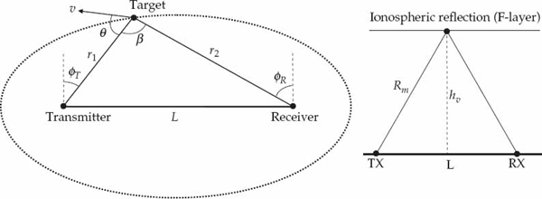
FIGURE 5.29 The diagram on the left shows a plan view of the bistatic radar scattering geometry for a surface target. The transmitter and receiver are separated by a distance L, the bistatic angle at the target location is β, while the total path-length of the target echo is r1 + r2. The measured group-range of the echo (r1 + r2)/2 locates the target on the ellipse, while the echo angle of arrival ϕR determines the position of the target on the ellipse. The diagram on the right shows a side-on view of a near vertical incidence ionospheric clutter path for the bistatic radar configuration. A single F-layer reflection with virtual hv and total (direct-wave) path length Rm is illustrated.
While assessing the relative merits of monostatic and bistatic HFSW radar configurations, one needs to consider the impact of different viewing geometries on the expected Doppler spectrum characteristics of the target echo and sea clutter for the intended HFSW radar coverage and mission priorities. This is because viewing geometry can significantly affect target detection and tracking performance for a certain mission type and coverage area (Wang, Dizaji, and Ponsford 2004). With reference to Figure 5.29, the bistatic Doppler shift of a target echo (defined as the group-range rate) is given by fD in Eqn. (5.87), where λ is the radio wavelength and v is the target speed. On the other hand, the Doppler shifts of the Bragg lines is given by fB in Eqn. (5.87), where β = ϕT + ϕR is referred to as the bistatic angle. For a given baseline L, Eqn. (5.87) implies that the Bragg lines are spaced closer together in Doppler frequency as the bistatic angle increases. This explains why the Bragg line separation in Doppler frequency narrows for a bistatic system as the group-range decreases. Indeed the Bragg-lines are observed to merge (at zero Doppler frequency) in a bistatic system as the group-range tends to that of the direct wave, i.e., when β = π.

(5.87)
A key point is that optimizing the radar configuration for a particular deployment needs to take into account the anticipated speeds and headings of the targets of interest with due regard to the characteristics of land and ocean surfaces in the surveillance area, including the synoptic behavior of surface-currents and the directional wave-height spectrum. Evaluating the probability of detecting target echoes against first- and second-order sea clutter using such information represents an important input for optimizing HFSW radar design and viewing geometry. A poor choice of radar configuration (and sites) can significantly degrade the capabilities of an HFSW radar system (Anderson 2007).
The group-range and angle-of-arrival distributions of ionospheric clutter also differ for monostatic and bistatic systems. The sketch on the right in Figure 5.29 illustrates that the group-range Rm/2 of the NVI ionospheric clutter path is approximately related to the inter-site separation L and virtual height of signal reflection hv by Pythagoras’ theorem, assuming a relatively short baseline length L (under 200 km). The influence of site separation on the coverage of an HFSW radar contaminated by NVI ionospheric clutter from the nighttime F-layer was analyzed in Leong (2006). It was concluded that a bistatic configuration can potentially allow the detection of ships at greater ranges than a monostatic system at night when ionospheric clutter is limiting. It was also argued in Leong (2006) that the elliptical constant group-range contours of a bistatic HFSW radar are more suitable for the surveillance of areas near water entries along coastlines.
5.4.1.2 Site Selection
A critical requirement for HFSW radar is to effectively couple vertically polarized signals (transmitted and received by the system) to the surface-wave propagation mode. A major factor influencing the coupling of radio wave energy to the surface-wave mode over the sea is the position of the antenna element(s) relative to the highly conducting saline water surface. Specifically, the height of the antennas above sea level and the distance of the antennas from the shoreline represent important criteria for HFSW radar site selection. This is because transmit and receive sites located on or very close to the coastline are necessary to effectively couple the ground-plane of the antenna to the ocean surface.
Ideally, the antennas should be placed as near as possible to the high-tide water mark to improve coupling of transmitted and received signals to the surface-wave mode. Locating the antennas even one or two wavelengths above sea level can introduce appreciable site losses (Berry and Chrisman 1966). The deleterious effect of antenna height on path loss has been validated in experiments. It has been found that raising the transmit antenna height by 35 m above sea level (with the receiver at sea level) results in an additional loss of approximately 6 dB over a one-way 140-km path. Elevating the antenna by a further 35 m incurred practically no additional penalty (Anderson et al. 2003).
An HFSW radar receive site typically requires relatively straight stretches of coastline at least 200–500 m in length to accommodate the major dimension of the antenna array. A receive site approximately 50-m wide is required to account for the antenna doublet separation, the length of ground radials and an isolation corridor. This translates to about 10–40 thousand square meters of coastal real estate. In addition, a site with relatively even topography and uniform ground electrical properties is preferable, particularly to minimize sources of array calibration errors. The combination of the above-mentioned factors often implies that HFSW radar site selection is heavily constrained in practice. Remote sea-state sensing systems, such as CODAR, utilize compact antennas that occupy a much smaller footprint, which significantly eases site constraints.
The HFSW radar receiver site should be well isolated (i.e., sufficiently distant) from residential and industrial areas to reduce the spectral density level of man-made noise below that of atmospheric noise in the lower HF band. If possible, it is also preferable for an HFSW radar system not to be located in regions of concentrated thunderstorm activity, where background noise levels tend to be higher. The impact of interference and noise at the site location additionally depends on the angular coverage of the receive beams steered for surveillance with respect to the directions of dominant sources, as well as the ability of these sources to reach the radar via ground-wave or skywave propagation. The large variability in ionospheric conditions with magnetic latitude and time of day also needs to be considered for site selection, as the occurrence and severity of Doppler-spread ionospheric clutter depends strongly on both of these factors.
HFSW radars operate effectively over open ocean areas, particularly in regions where water salinity is high and where high sea-states occur less frequently. Surface roughness can significantly attenuate the surface-wave signal, especially at frequencies near the middle of the HF band. High sea-states also increase the received surface-clutter power in Doppler intervals where slow-moving target echoes need to be detected. The impact of local bathymetry on the received clutter properties, including dominant ocean currents and tides in the coverage, should be considered when selecting the radar site(s). Careful attention also needs to be paid to the presence of land masses or islands, particularly those which are wide or long and close to the transmitter or receiver, as surface-wave attenuation can be significantly increased by propagation over significant stretches of terrain. The relatively lower conductivity of fresh-water lakes, or inland seas where ocean water mixes with fresh water, may preclude the effective operation of HFSW radar systems. For this reason, sites looking out to open ocean but adjacent to significant outflows of fresh water may be sub-optimal.
HFSW radars are almost always land-based systems. However, there has been considerable interest in evaluating the feasibility of mobile shipborne HFSW radar installations. Because of the long radio wavelengths in the lower HF band, the entire ship will radiate as the antenna, which can degrade the resulting antenna gain and radiation pattern properties. Mutual electromagnetic interference (EMI) with other shipboard systems is also a significant issue. An electromagnetic compatibility (EMC) study was conducted in Li et al. (1995) for the case of HF antennas mounted on a Navy ship. An experimental analysis of HFSW radar sea clutter received on a moving platform appears in Xie, Yuan, and Liu (2001). The possibility of fielding multistatic systems involving shipborne sites has been discussed in Baixiao et al. (2006).
5.4.2 Radar Subsystems
An HFSW radar is composed of three main subsystems; the transmit system, the receive system, and an HF spectrum occupancy monitor for clear channel advice. The latter, which may be regarded as being part of the receive signal processing system, is not described here as it was previously discussed in for skywave OTH radar as an element of the frequency management system. As there is also considerable overlap between the main subsystem design concepts for skywave OTH and HFSW radar, topics such as transmit/receive antenna/array design, and signal processing will be covered briefly here.
5.4.2.1 Transmit System
Skywave OTH radars have been implemented using antennas with vertical or horizontal polarization, as ionospheric propagation is supported for both, but the polarization of an HFSW radar transmit antenna must be vertical to effectively support surface-wave propagation at OTH ranges. Regarding the choice of transmit antenna element, the main aspects of concern are antenna efficiency over the design frequency range, azimuth coverage to floodlight the surveillance area, high gain at low elevation angles for effective coupling to the surface-wave mode, low gain at high elevation angles to reduce illumination of skywave clutter sources, and adequate front-to-back ratio for systems that only look for targets in a forward direction.
Other important considerations include the susceptibility of the antenna structure to Aeolian noise caused by mechanical vibration induced by winds, which may be strong in coastal regions, the capability to radiate HF signals at the required power levels without significant distortion due to arcing and other nonlinear phenomena, as well as cost and ease of deployment in the field. A ground screen, radial wires, or counter poise is typically used to improve the low elevation angle gain of the antenna.
A number of past and present systems, including the high-power site of the Iluka HFSW radar, have selected the vertical log-periodic dipole array (LPDA) as the transmit antenna element. For maximum efficiency in the 5–15 MHz frequency range, resonant antenna elements need to be large structures. The radiating elements of an LDPA antenna may be 10–40 m high and require an area of about 200-m by 200-m to install, including the supporting structure, ground screen, and equipment compound. An HFSW radar using a single LPDA transmit antenna floodlights the entire coverage area with a relatively broad beam that may be 90–120 degrees wide in azimuth (at low elevation angles). Unlike skywave OTH radars, this permits the entire surveillance area to be illuminated simultaneously at the expense of reduced sensitivity in a noise-limited environment. HFSW radar systems based on multiple transmit antenna elements and a digital waveform generator per element architecture that facilitates electronic beam steering have also been developed and will be described in the final section of the chapter.
The average transmit power of HFSW radar systems designed for surveillance up to the EEZ limit is typically between 1 and 10 kW. Solid-state devices offer an attractive alternative to vacuum tube amplifiers in HFSW radar applications that demand operation over a wide frequency band with rapid frequency changes. For example, this capability is desirable to enable dual-frequency operation by generating interleaved radar pulses centered at two widely spaced operating frequencies (Leong and Ponsford 2004). By comparison, HFSW radars used for remote sea-state sensing typically transmit an order of magnitude lower power. For example, the low-power site of the Iluka HFSW radar was based on a simple dart antenna with a 100-W transmitter, while other low-power systems such as OSMAR have used a three-element YagiUda antenna driven by a 200-W power amplifier.
When an HFSW radar is surrounded by ocean (e.g., located on a narrow peninsula or mounted on a ship), transmit antennas with a good front-to-back ratio are important to reduce scattering which occurs from behind and then in front of the transmit location. This mechanism, referred to as the second part of second-order clutter (Ponsford 1993), can significantly raise the “wings” of the clutter Doppler spectrum in the frequency region outside of the Bragg lines. This adversely affects the detection of slow-moving targets by an amount that depends on sea-state and viewing geometry. The experiments described in Ponsford (1993) show that a figure-of-eight transmit antenna pattern increased the clutter spectral density at Doppler frequencies outside of the Bragg lines by 9 dB compared to a cardioid pattern for an HFSW radar largely surrounded by sea.
Two-site HFSW radar systems have predominantly used signals based on the repetitive linear FM continuous waveform. A constant-modulus waveform with unit-duty cycle not only maximizes the average power for a given transmitter peak-power rating, but also places less stringent demands on the linearity of power amplifiers. The repetitive linear FM continuous waveform can also maintain excellent ambiguity function properties after temporal or spectral tapering is applied to reduce out-of-band spectral emissions. Moreover, computationally efficient matched filtering techniques may be applied to such waveforms, as described in Chapter 4.
On the other hand, single-site systems have exploited sequences of phase-coded pulse waveforms, such as binary or Frank quadrature phase codes (Ponsford, Dizaji, and McKerracher 2003). The phase codes used in successive pulses of the CPI can be changed to mitigate range-ambiguous (second-time-around) radar echoes scattered by long-range (skywave) clutter sources. In any case, effective Doppler processing in HFSW radar requires high spectral purity of the radiated waveform. Phase noise characteristics better than 80–100 dBc/Hz at 1 Hz from the carrier are often necessary to avoid instrumental (as opposed to physical) limitations to system performance.
5.4.2.2 Receive System
The majority of HFSW radars used for surveillance have adopted a receive antenna based on a uniform linear array (ULA) of vertically polarized singlet, doublet, or quadruplet monopole elements. With respect to 2D arrays, the widespread use of the ULA geometry in HFSW radar systems is motivated by the relatively simpler array calibration and data processing, as well as the ease of deployment on straight stretches of coastline, where the array may be oriented along the shore with boresight perpendicular to the water’s edge. For example, the Australian Iluka system was based on a ULA of 32 monopole antennas with an aperture of 500 m and a digital receiver per element architecture. Such a ULA provides a receive beam with a main lobe about 5 degrees wide in azimuth at an operating frequency of 6 MHz. Two dummy elements (not connected to a receiver) are often placed at either end of the ULA to improve the homogeneity of mutual coupling, particularly for the first and last receiving elements.
The receive antenna elements do not need to be as well-matched over the design frequency range as the transmit element. The main justification for this is that the radar operates in an externally noise-limited environment (presumably with little or no spatial structure). In this case, a well-matched receive antenna element increase the gain for radar signals and external noise by the same amount, which yields no improvement in SNR. The use of (relatively short) monopole elements on receive significantly reduces the cost and footprint of the antenna array, besides being more robust to Aeolian noise. However, it has been argued that more efficient (broadband) antenna elements on receive may improve SNR when the external noise field exhibits significant spatial structure and adaptive beamforming is used.
Ideally, the receive antenna element needs to provide high gain at low elevation angles over a wide azimuth sector (equal to that of the coverage), an appropriate front-to-back ratio for a forward-looking ULA, and a broad null for signals arriving at near-vertical incidence. An ideal vertical monopole antenna on a perfectly conducting ground plane has an omnidirectional pattern in azimuth and a maximum gain at grazing incidence. The gain decreases with increasing elevation and approaches zero near vertical incidence. A ULA based on vertical monopole antenna elements arranged as doublets (separated by about 15 m to provide adequate front-to-back ratio in the lower HF band) over a ground mesh-screen, which stabilizes the input impedance of vertical radiators and improves coupling of the antenna ground-plane to the surface-wave mode, represents a cost-effective solution that is consistent with the aforementioned objectives.
The ground screen is typically placed both under and in front of the receive array. In an attempt to increase antenna gain at low elevation angles, certain HFSW radar systems have used ground screens that extend all the way into the sea. On the other hand, low gain at high elevation angles is required to attenuate ionospheric clutter received via the NVI path. In practice, antenna design is not sufficient to eliminate the intense overhead and near-overhead echo, or the reception of skywave interference and noise, as such signals may be incident over a range of elevation angles. The combination of antenna design, frequency management, and signal processing is required to reduce performance limitations imposed by skywave disturbance signals in real-world systems.
In addition to the main (vertically polarized) antenna elements in the receive array, a number of auxiliary antennas with horizontal polarization may be incorporated to augment the receive array (possibly in two dimensions). Since ionospheric clutter and interference signals arriving via the skywave mode are elliptically polarized, the auxiliary antennas can, in principle, be used to cancel ionospherically propagated disturbances received by the main array using polarization filtering. This topic will be discussed in the next section with application to interference rejection. Although two-dimensional arrays, such as L-shaped and T-shaped geometries, have the potential to yield superior performance against clutter and interference received via the skywave mode, no currently operational HFSW radar system designed with surveillance as its primary mission has been implemented with this feature to date.
In state-of-the-art HFSWR radar systems, the classic superheterodyne receiver has been superseded by direct digital receivers (DDRx) that can sample the entire HF band at the antenna element after a bandpass preselect or filter. Multiple narrowband frequency channels can be digitally down converted and low-pass filtered to enable simultaneous multi-frequency operation as well as other radar support functions such as common aperture environmental noise monitoring. As far as adaptive processing is concerned, the DDRx architecture is relatively less susceptible to degradations in spatial dynamic range of the antenna array caused by nonidentical reception channel transfer functions (frequency responses), which often occurs in the selective (analog IF) sections of a classical superheterodyne receiver.
5.4.3 Signal and Data Processing
The rudimentary conventional signal- and data-processing steps described for skywave OTH radar in the previous chapter also apply to HFSW radar. The pulse compression, array beamforming, and Doppler processing steps follow identical principles, so these will not be repeated here. The main differences in relation to system resolution and accuracy are briefly summarized. Two signal-processing applications specific to HFSW radar that have not been discussed in detail so far will be described; namely, the mitigation of NVI ionospheric clutter mitigation by adaptive processing, and the rejection of skywave interference by polarization filtering. CFAR and tracking techniques that show promise for HFSW radar are also identified.
The surface-wave mode is more frequency-stable than skywave propagation, which allows much longer CPIs to be gainfully employed in HFSW radar. This is particularly important for the detection of large surface vessels, where the target velocity also tends to remain steady for long periods of time. In many HFSW radar systems, the transmitter floodlights the whole coverage simultaneously such that the CPI equals the revisit rate. Relative to a step-scanning transmitter, which steers the beam to different directions in the coverage, this allows for greater time-on-target and Doppler-frequency resolution for a given revisit rate, which may improve detection performance in a clutter-limited environment. Ship-detection CPIs may extend into the hundreds of seconds in HFSW radar, while aircraft-detection CPIs typically range from 2 to 10 seconds.
The surface-wave mode is also less frequency-dispersive than the skywave mode. In principle, this allows radar bandwidths of up to 100 kHz or more to be employed for fine range resolution (1.5 km). The physical limitation imposed by the coherence bandwidth of the propagation channel is much less restrictive for an HFSW radar than for a skywave OTH radar. However, high user-congestion in the lower HF band often constrains the maximum group range resolution to about 5 km (30 kHz) in practice. While the range and Doppler resolutions of an HFSW radar are typically higher than a skywave OTH radar, the angular resolution is comparatively lower due to the relatively smaller receive apertures and typically lower operating frequencies. The receive beams may have half-power main lobe widths of about 5–10 degrees. This provides a cross-range resolution of roughly 4–8 km at a range of 50 km, and about 25–50 km at a range of 300 km.
It is also important to distinguish between the spatial resolution cell size and target localization accuracy. Provided the target echo is well resolved from other radar echoes in at least one of the three radar processing dimensions (azimuth, range, or Doppler), the localization accuracy of a target echo with high signal-to-noise ratio may be 5–10 times greater than the resolution in each processing dimension when the peak coordinates are estimated by interpolation between the highest amplitude sample and its two immediate neighbors. A salient point is that the high Doppler resolution of an HFSW radar can indirectly enhance the accuracy of target echo location estimates in range and azimuth by resolving a high SNR target echo from clutter returns and other target echoes.
Several CFAR techniques tailored specifically to the HFSW radar signal environment have been proposed and tested, using real data where an individual CPI may have more than one million pixels. The reader is referred to Wang, Wang, and Ponsford (2011) and Lu et al. (2004), as well as Dzvonkovskaya and Rohling (2006) and Dzvonkovskaya and Rohling (2007), and references therein, for specific details of CFAR implementations and their application to real data. After CFAR processing, a plot extractor detects and estimates the parameters of all peaks in range, azimuth, and Doppler that exceed a predetermined threshold and forwards the extracted “hits” in each CPI to a tracker where successive detections are associated to form tracks. The tracker needs to filter out many false alarms over time to keep the false track rate low while maintaining an appropriate probability of detection.
The multiple-hypothesis tracker (MHT) has been successfully implemented in some operational HFSW radar systems. As explained in Ponsford, Sevgi, and Chan (2001), this tracker incorporates a deferred decision approach by maintaining multiple track options over a number of updates until enough confidence is built up to establish a track and remove the other competing alternatives. The minimum number of associated detections required to confirm a track is normally limited by the requirement to maintain a low false track rate.
The output of the track validation procedure is the declaration of a set of confirmed tracks that have satisfied the track promotion logic (e.g., two associated detections for tentative, five associated detections for confirmed, and seven misses to delete). Most false tracks arise due to ionospheric clutter and ocean clutter peaks. False track rates better than 0.25 per hour are quoted in Ponsford, Dizaji, and McKerracher (2003) in an experiment where the system successfully tracked all reported targets.
With respect to skywave OTH radar, coordinate registration is a simpler problem in HFSW radar due to the greater certainty regarding the surface-wave propagation path. For an established track, track accuracy is typically better than 0.5 km in range and 0.25 degrees in azimuth (Ponsford, Dizaji, and McKerracher 2003). Track position errors are often dominated by system biases that can be removed by calibration. In addition, a target normally produces a single surface-wave echo as opposed to a number of well-resolved echoes, which commonly occurs due to multipath in the skywave propagation channel. This effectively eliminates the multiple track to target assignment problem present in skywave OTH radar systems.
5.4.3.1 Ionospheric Clutter Mitigation
Adaptive processing may be combined with multi-frequency operation as well as receive and transmit antenna design as part of an overall ionospheric clutter mitigation strategy. In the absence of experimentally validated signal-processing models for ionospheric clutter, a number of empirical observations of this phenomenon are useful for guiding adaptive processor design. The NVI ionospheric clutter signals that cause significant problems for HFSW radar beyond ranges of about 90 km are typically distributed in range-Doppler and are time-continuous over the CPI. For this reason, spatial and space-time adaptive processing have been identified as the main classes of signal processing techniques to mitigate this disturbance type.
Although it may be anticipated that ionospheric clutter received in a particular range cell will exhibit a degree of directionality, it is perhaps less expected that the spatial structure of ionospheric clutter can change significantly from one range cell to next. In other words, the spatial characteristics of ionospheric clutter in the coverage are often found to be highly heterogeneous in range. This has a number of implications for adaptive filter design. First, the adaptive filter needs to be updated on a range-by-range cell basis with training data taken only from the operational range cell to be processed. This means that no “target-free” (supervised) secondary data is available for training the adaptive filter when all the pulses in the CPI or Doppler cells are used to estimate the disturbance covariance matrix.
The combination of unsupervised training data and finite sample support slows convergence rate and leaves the target highly susceptible to self-cancelation, particularly in the presence of array calibration errors. If the presumed useful signal response vector does not accurately match the actual (received) one, the target is interpreted as a disturbance by the adaptive processor and consequently canceled. Second, the training data may also contain powerful first-order ocean clutter that does not need to be rejected by the adaptive filter since these returns are effectively dealt with by Doppler processing. The presence of powerful sea clutter in the training data can seduce the adaptive filter into canceling surface returns in preference to the ionospheric clutter, which consumes adaptive degrees of freedom without providing significant benefits.
For this reason, post-Doppler techniques have been adopted such that only Doppler cells free of dominant sea clutter returns are used for training (Abramovich, Anderson, Lyudviga, Spencer, Turcaj, and Hibble 2004). However, a potential problem stems from the fact that the most energetic ionospheric clutter components often occupy the “low speed” Doppler cells, where second-order sea clutter and target echoes also reside. Moreover, the heterogeneity in angular distribution of ionospheric clutter may not be confined to the range alone, but may also be present across Doppler cells. This can lead to performance losses when the Doppler cells used for training at a given range are different to the ones processed by the adapted filter. The effectiveness of post-Doppler techniques also degrades when the ionospheric clutter in a particular range is associated with a non-stationary angular distribution over the relatively long HFSW radar CPI. An alternative pre-Doppler technique for ionospheric clutter mitigation has been proposed in (Fabrizio and Holdsworth 2008).
5.4.3.2 Polarization Filtering
Skywave interference is elliptically polarized, in general, and can therefore be received by antennas with vertical and horizontal polarization. On the other hand, only vertically polarized antenna elements are expected to receive the radar signal propagated by the surface-wave mode. Adaptive polarization filtering to suppress skywave interference was applied in a practical HFSW radar by Madden (1987) using a single auxiliary antenna with horizontal polarization. Another experimental investigation incorporating up to four horizontal dipoles configured as two separate crosses behind a main array of six vertically polarized elements was conducted in Leong (1997).
In practice, the radar signal is unfortunately not completely absent from the outputs of the horizontally polarized antennas due to imperfections or misalignment of these elements. For effective adaptive polarization filtering, the presence of surface clutter and target echoes in the auxiliary antennas needs to be minimized. The horizontal antennas therefore need to be carefully designed and installed to minimize the reception of the useful signal. The sample matrix inverse (SMI) method was used in Leong (1997) to estimate the adaptive processor weights in each waveform repetition interval by taking training samples from the farthest range bins (i.e., near the end of the pulse repetition interval), which contained skywave interference but minimal surface-wave clutter.
It was found that system performance improved with the use of an increasing number of horizontal antennas. Interference suppression levels greater than 13 dB were achieved using four horizontal antennas in Leong (1997). For systems based on two auxiliary antennas, configurations using orthogonally oriented horizontal dipoles performed the best. In this case, the location of the dipoles appeared to have little effect on performance (i.e., whether the orthogonal antennas were separated or colocated). Use of only one horizontal dipole antenna achieved about 4–6 dB interference suppression, depending on the orientation of the horizontal element.
Performance when using vertical and horizontal antenna elements as the auxiliaries was also compared in Leong (2000). When the target echo and interference are incident from a similar direction, the target echo is canceled along with the interference when only vertical monopoles were used as auxiliary elements. This is because the null formed on the interference also cancels the target. However, the target echo could be protected (i.e., not canceled) in the main beam interference scenario when the horizontal antennas were used as auxiliary elements. This result, which represents an important benefit sought from spatio-polarization filtering, was achieved despite the Bragg lines being visible at the outputs of the horizontal antennas (6–8 dB lower than those observed in the vertical antennas).
The study concluded that the interference was not suppressed as effectively when using horizontal (as opposed to vertical) antennas as the auxiliaries. This is because the skywave interference received by the main array of vertical antennas is better correlated with the interference received by the auxiliary vertical antennas than that received by the horizontal antennas. A similar observation was reported in an independent experimental study that used 16 elevated-feed vertical monopoles and 16 horizontal-loop antennas in a ULA that was approximately 300-m long (Abramovich, Spencer, Tarnavskii, and Anderson 2000).
5.5 Operational Considerations
For optimum performance, HFSW radar operation needs to be tailored to the target class of interest, the range-Doppler region where the target echo is expected, and the prevailing environmental conditions, where the latter includes sea-state and ionospheric structure, as well as HF spectrum occupancy and background noise spectral density. Similar to skywave OTH radar, the appropriate choice of carrier frequency is of fundamental importance to the successful operation of HFSW radar. The carrier frequency effectively controls the tradeoff between several competing factors that strongly influence target detection and parameter estimation performance. Specifically, carrier frequency selection impacts surface-wave path loss (as a function of range), target RCS characteristics, ocean and ionospheric clutter properties, background noise spectral density, as well as system gain and azimuth resolution.
The first part of this section reviews a number of basic RCS concepts relevant to HFSW, where the dominant component of polarization is constrained to be vertical, and coupling of the target with the sea surface cannot be ignored for surface vessels and low-altitude aircraft. For a comprehensive treatment on the topic of RCS, the reader is referred to Knott, Shaeffer, and Tuley (1993) and Ruck, Barrick, Stuart, and Krichbaum (1970). The second part of this section describes the main criteria used for frequency selection in HFSW radar and explains the significant advantages of dual or multi-frequency operation, which have been exploited in a number practical systems. The third part of this section contrasts the designs and capabilities of three representative HFSW radar systems with different architectural characteristics.
5.5.1 Radar Cross Section
The RCS of a target, such as a ship or aircraft, depends on many factors, including target dimensions and structure, electrical properties of construction materials, illumination frequency, viewing geometry, and the polarization(s) used on transmit and receive. The target RCS appears in both the noise and clutter-limited versions of the radar equation. Realistic estimates of target RCS are therefore valuable for calculating the energy budget required to satisfy performance requirements at the radar design stage, or for predicting the detection performance of a given system against a particular target class.
A detailed knowledge of RCS characteristics may also assist to determine the most favorable operating mode to detect a certain type of target. Moreover, an understanding of RCS signatures in the frequency and/or polarization domains may be exploited as a discriminant for target classification (Strausberger, Garber, Chamberlain, and Walton 1992). Information regarding the expected target RCS fluctuations may also help to determine the potential value of using echo amplitude as an additional parameter for associating detections in a tracking system. Considerable effort has therefore been invested to model and measure the RCS characteristics of surveillance radar targets.
In skywave OTH radar, targets are illuminated by a signal with time-varying polarization due to (non-stationary) Faraday rotation in the ionosphere. In this case, various structures on the target, such as the wings or fuselage of an aircraft, can at different times contribute in a dominant way to the overall RCS as the rotating polarization becomes more or less matched to different canonical structures on the target. The situation is not as general for HFSW radar because surface-wave propagation is only effectively supported for vertical polarization, both to and from the target. Consequently, the received echo is primarily a result of scattering from vertical (conductive) elements of the target structure. The RCS of maritime vessels is therefore particularly sensitive to the target’s height above the sea surface.
The presence of metal masts or frames that effectively increase the vertical extent of a maritime vessel have the potential to significantly increase RCS when the surface-wave mode alone is active. For example, it is shown in Trizna (1982) that the RCS of a small surface vessel (fishing boat) is dominated by the quarter wavelength monopole contribution of a 16.6-meter-long metal mast with a peak RCS near 30 dBsm at the resonant frequency of 4.5 MHz. Owing to the characteristics of this element, the RCS drops rapidly to values below 10 dBsm at frequencies spaced 1 MHz either side of the resonant frequency. The vertical polarization of the surface-wave means that the illumination frequency and viewing geometry play prominent roles in defining the target RCS feature space in HFSW radar (Wu and Deng 2006).
5.5.1.1 Rayleigh-Resonance Region
The RCS characteristics of a target are highly dependent on the major dimension D of its conductive segments relative to the radar wavelength λ. Broadly speaking, there are three scattering regimes where both qualitative and quantitative differences in RCS behavior occur. The low-frequency regime, where the target dimensions are much less than the radar wavelength, is known as the Rayleigh scattering region (D  λ). The intermediate frequency regime, where the target dimensions are of the same order as the radar wavelength, is referred to as the resonance or Mie scattering region (D ≈ λ). The high-frequency regime, where the target dimensions become much larger than the radar wavelength, is called the optical scattering region (D
  λ). Although the resonance region may be approximately regarded as the frequency interval where 0.1 ≤ λ/D ≤ 10, there are no distinct boundaries between the different scattering regimes. From a physical perspective, the RCS characteristics of a target transition gradually from those of one regime to another as the frequency changes.
HFSW radars typically operate in the lower HF band (3–15 MHz), which corresponds to a wavelength range between 20 and 100 m. At such frequencies, most aircraft and surface vessels have a major dimension comparable to the radar wavelength, which places their RCS in the resonance scattering region. More precisely, the RCS characteristics of large (ocean-going) ships lie in the resonance region over the entire HF band. However, the smallest aircraft, cruise missiles, and go-fast boats have RCS characteristics that fall within the Rayleigh region near the low end of the HF band.
In the Rayleigh region, the RCS is strongly influenced by the target’s gross dimensions as opposed to its detailed structure or shape. It also exhibits reduced sensitivity to viewing geometry. The RCS of a target illuminated at low frequency has characteristics that become more like an isotropic scatterer. Perhaps most importantly, the target RCS decreases rapidly with the fourth power of frequency (to a good approximation) in the Rayleigh region.
In the resonance region, a number of different elements (conductive segments) on the target may contribute in a significant way to the resultant RCS. Depending on the radar viewing geometry and the relative positions of the dominant scatterers on the target, the resultant RCS may fluctuate significantly with aspect angle at a fixed operating frequency. On the other hand, the vector sum of scattered contributions from different elements of the target may interfere in a constructive manner at one frequency and destructively at another for a given radar viewing geometry and target aspect angle. This causes the target RCS to exhibit peaks and troughs (strengthen or weaken) within a confined range as the operating frequency is changed. The backscatter target RCS, and hence echo power received by a monostatic HFSW radar, can vary significantly (by more than 10 dB) as a function of target aspect and illumination frequency in the resonance region.
Estimates of the free-space target RCS may be suitable in certain radar applications, particularly for systems operating at UHF and microwave frequencies. In the lower HF band, coupling between the highly conductive sea surface and a surface-vessel cannot be ignored as far as the impact on effective target RCS is concerned. In addition to the approximate image field resulting for a surface-vessel on a calm sea surface, ocean roughness and surface-vessel motion can have an appreciable influence on the effective target RCS observed by an HFSW radar. Target RCS signatures in both aspect angle and illumination frequency have been simulated for the case of a stationary surface vessel over a calm sea, as described in the next section. Modeling of the target RCS becomes more difficult when vessel motion (including pitching and rolling) is introduced and different sea-state conditions are considered.
The radar cross section of large vessels (>1000 tons) at HF exhibits quite complex behavior, but the angle-average value may be roughly approximated by the empirical formula σ = 52 f D3/2, where σ is the vessel’s free-space RCS in square meters, f is the radar frequency in MHz, and D is ship size in thousands of metric tons. The RCS of small and medium-sized vessels (< 1000 tons) is dominated by their vertical metallic superstructure. If this superstructure is grounded to the ocean surface, or isolated from the ground, then the RCS of the vessel can be approximated by that of a grounded monopole antenna, or dipole antenna, respectively.
A resonant dipole has an RCS that approaches λ2, while the RCS of an equivalent resonant monopole is 6 dB lower. The RCS below resonance may be assumed to exhibit an f4 roll-off. Due to the large (decameter) wavelengths at HF, small boats with a low vertical extent will have very small RCS. Such targets may only be detected against background noise, which requires their radial speed to be high enough for the echo to be resolved in Doppler frequency from the ocean clutter.
5.5.1.2 Modeling Approaches
Analytical techniques based on geometrical optics, physical optics, or the geometrical theory of diffraction may be used to provide rough estimates of RCS values provided the target can be modeled reasonably well in terms of a few simple canonical structures. The RCS characteristics of simple structures including a perfectly conducting cylinder, monopole element, and hemisphere, are illustrated in Skolnik (2008b).
For more precise modeling of target RCS, it is often necessary to resort to numerical methods. In this case, finite-difference time-domain (FDTD) or method-of-moments (MOM) techniques may be employed to compute RCS estimates. These numerical techniques employ time and frequency domain formulations, respectively, to provide full-wave solutions of Maxwell’s equations in three dimensions.
A popular program based on the MOM formulation is the numerical electromagnetic code (NEC). There are several versions of NEC, with NEC-2 (1981) being the latest version of the code that is openly available. To imitate complex metal structures, actual design drawings of an aircraft or ship are often used to construct a wire-grid model of the target. Meshing is typically assumed to be composed of perfect electric conductor (PEC) material and specific criteria are followed regarding the choice of grid spacing and wire radius for a given segment length in the target model. An example comparing experimentally measured and simulation results for the RCS of a large surface vessel using NEC-2 will be illustrated below.
Numerical RCS modeling should not only account for the complex target structure, but also its interaction with the ocean surface. Wire mesh models of a surface-vessel are typically attached to an infinite PEC ground plane to simulate a flat and perfectly conductive ocean surface. This attempts to capture the scattering influences from the target’s image as well as any potential coupling. An alternative is to compute the target free-space RCS with the wire grid model connected to its reflection in the horizontal plane. Incorporating ocean roughness and dealing with dynamic target interactions with the water surface is more difficult, as is the modeling of targets that do not have highly conductive surfaces. To validate simulated RCS estimates, it is common to compare results obtained using different numerical techniques, or to reconstruct complex models of targets with already available (experimentally measured) RCS values.
5.5.1.3 RCS Interactions
The spatial resolution cell size of an HFSW radar is very large compared to the dimensions of a target, so it often occurs that a single range-azimuth resolution cell contains more than one target. In this case, mutual RCS interactions between unresolved targets may be significant from a detection or classification viewpoint. In practice, the effect of RCS interactions becomes most noticeable in an HFSW radar when echoes from different targets occupy the same range-azimuth and Doppler cell, as in the case of nearby stationary targets, for example.
In Sevgi (2001), strong signal-strength fluctuations have been observed on the echo from an off-shore oil platform on the Canadian East Coast due to the presence of shuttle tankers that stop close to the platform for loading. The oil rigs are over 100 m high and have an RCS in the order of 50 dBsm, while the tankers in the proximity of the oil rig are some 400 m in length and have an angle-averaged RCS of approximately 40 dBsm. The usually steady echo from the oil rig can vary by more than 10 dB due to the presence of the tanker. Echo power fluctuations caused by mutual RCS interactions effects typically exhibit different fading characteristics with respect to those expected for a single maneuvering) target. This may potentially be used to infer the presence of multiple targets in the same radar resolution cell.
The concept of exploiting RCS coupling for the detection of a target behind a second target via forward scattering from the latter has been considered in Guinvarch et al. (2006). The authors speculate that a collection of large vessels queued in the vicinity of each other around a congested port or in a narrow strait can form an “electromagnetic barrier” to conventional X-band coastal radars, which may preclude the detection of smaller targets located in the shadow regions. The shadow regions are less pronounced in the HF band, provided the considered location is not immediately behind the large vessel.
While the backscatter RCS tends to dominate at low frequencies, it has been observed that the forward scatter RCS begins to dominate as the frequency is increased. A study in Solomon, Leong, and Antar 2008 demonstrated that out of all the bistatic angles, forward scattering yielded the most potential for matching or exceeding the monostatic (backscatter) RCS values above a certain frequency regardless of the target aspect angle. For the large surface vessels considered, the relative increase in RCS reached as high as 30 dB with the broadside target aspect being the only orientation that maintained equivalence between the forward/backscatter RCS and did not show an increase at higher frequencies. Although this trait existed over the entire HF band for very large vessels, this feature engaged at different frequency points for smaller vessels, after which the forward scattering advantage was consistently maintained.
5.5.1.4 Experimental Measurements
While the RCS of ships and aircraft have been extensively studied in the optical region, only a limited number of investigations have been conducted in the HF band. Empirical expressions derived for the free-space RCS of vessels at microwave frequencies may not translate accurately to those observed by an HFSW radar. For example, RCS expressions based solely on vessel gross-tonnage and radar frequency do not explicitly consider the significance of vessel height or the influence of the conductive sea surface on RCS for HFSW radar.
Field experiments to measure RCS in the HF band may be conducted by using natural reference scatterers with known RCS, such as Bragg lines in a fully developed sea (Leong 2006), or reference signals from well-calibrated transponders with an identifiable Doppler offset located in the same area as the target (Dinger et al. 1999). When attempting to measure the dependence of RCS on target aspect, the range of the vessel needs to be sufficiently small such that the echo can be reliably detected above the background disturbance level even when the RCS passes through potentially deep nulls.
The HF-RCS of large and small ships illuminated by the surface-wave mode were studied in Leong and Wilson (2006). Specifically, RCS modeling results obtained by numerical simulation were compared with real measurements made by HFSW radar at frequencies of 3.1 and 4.1 MHz for two known vessels: a 2405-ton Canadian Coast Guard ship (Teleost) and a 36-kiloton cargo-freighter vessel (Bonn Express), both shown in Figure 5.30. The measurements were calibrated based on the assumption of a fully developed sea at the operating frequency, where the first-order scattering coefficient (echoing cross section per unit area) and the surface area of the radar resolution cell containing the test vessel are known.

FIGURE 5.30 The left panel shows the Bonn Express, a 36 kiloton cargo-container with a length of 236 m and an estimated bridge height of 30 m. The right panel shows the Teleost, a medium-sized (2405 ton) coast guard ship with length 63 m, breadth 14.2 m and maximum mast height of 24 m. © Crown 2010. Government of Canada. (Courtesy of Dr. H. Leong, Defence R & D Canada.)
Due to their different Doppler frequency shifts, the echo from the vessel may be separated and compared against the strength of the Bragg lines, which serve as a natural reference for making calibrated RCS measurements. This experimental method for estimating target RCS is appropriate when persistent winds with a sufficient speed and fetch fully develop the sea at the radar operating frequency. It is also convenient if the beam direction is close to being parallel with the mean wind direction when knowledge of the angular spreading function at the Bragg wave train frequency is not available. The lower the operating frequency, the less likely the sea will be fully developed due to the increasing wavelength and higher speed of the ocean waves responsible for producing the Bragg lines in the Doppler spectrum.
It was found that both vessels had a comparable angle-averaged RCS of approximately 40 dBsm at 3.1 and 4.1 MHz, despite the Teleost having a gross tonnage 15 times less than the container ship. This result was attributed to the large contribution of the A-frame on the Teleost, which at a height of 24 m is near the resonant quarter-wavelength height at 3.1 MHz. Figure 5.31 shows that NEC accurately estimated the measured RCS values for the Bonn Express at 4.1 MHz, including the dependence of RCS on aspect angle at points where experimental data was obtained. Close agreement between predicted and measured RCS values as a function of target aspect have also been reported for the Teleost in Podilchak, Leong, Solomon, and Antar (2009).
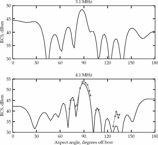
FIGURE 5.31 Radar cross section as a function of aspect angle for the Bonn Express cargo freighter at 3.1 MHz and 4.1 MHz. Numerical modeling results are shown with a solid line, while measured data are shown by the dots joined with a solid line. A dual-frequency HFSW radar would have a better chance of maintaining track at aspect angles near 62, 70, 100, 105 degrees. (© Crown 2010. Government of Canada. (Courtesy of Dr. H. Leong, Defence R & D Canada.)
The close agreement between experimental and simulated results in the bottom panel of Figure 5.31 provides convincing evidence that the backscatter RCS passes through peaks and troughs as a function of target aspect angle at a frequency of 4.1 MHz. A comparison of the modeling results in the top and bottom panels of Figure 5.31 predicts that the locations of these peaks and troughs differ significantly at carrier frequencies spaced 1 MHz apart at the lower extreme of the HF band.
For certain target aspects, the difference in RCS at these two frequencies can potentially enhance or reduce the received echo power by margins in excess of 10 dB. The dependence of target RCS over this frequency range may be exploited to improve detection performance by means of dual-frequency operation. As pointed out in Leong and Wilson (2006), the enhanced target RCS arising for a large vessel near broadside explains why vessels traveling tangentially have occasionally been detected at very long ranges by HFSW radars.
At one extreme, large ferry ships have measured RCS values approaching 50 dBsm (Menelle et al. 2008), while at the other, small boats with lengths ranging from 5 to 8 m typically have RCS values of 0–10 dBsm (or less) in the lower HF band. For operating frequencies between 3 and 5 MHz, the RCS of medium-sized vessels with a gross registered tonnage of about 1000 tons was estimated to be about 25–30 dBsm at aspects less than 25 degrees from the stern-on or bow-on directions (Leong 2007). In practice, mean RCS values should be interpreted with caution as the actual target RCS can vary by an order of magnitude or more relative to the mean in the resonance region depending on the combination of operating frequency and target aspect.
The detection and tracking of small surface-craft, also known as go-fast boats (GFB) (Dinger et al. 1999), or rigid inflatable boats (RIB) (Blake 2000), is of significant interest for border protection as their high speed, good endurance, and low vertical profile allows them to cover long distances very rapidly and covertly. Besides their low height (often less than 1 m above the sea surface), these boats are generally constructed with minimal metallic content. Depending on design and configuration, such targets may only have one or two significant conducting segments. Other materials, such as fibreglass and wood, are often used for the floor or hull, while plastic inflatable tubes may be used to provide buoyancy. This combination of attributes makes the detection of such vessels challenging for any type of radar, particularly when the sea is not calm.
A detailed experimental and simulation study of the RCS behavior of this target class appears in Dinger et al. (1999). The RCS of two go-fast boats was measured at bow-on and stern-on aspects with respect to the HFSW radar receiver as a function of operating frequency when the vessel speed was approximately 20 knots. For a 25-ft GFB, the RCS increased gradually from a value of about 0 dBsm at 6 MHz to 9 dBsm at 15 MHz. A 21-ft GFB exhibited a similar increase with frequency, but the RCS was 7 to 10 dB lower.
For both boats, no peaks or resonant structures were observed in the variation of RCS with frequency, which is consistent with Rayleigh scattering region behavior. In (Blake 2000), the RCS of a 5.4-m-long RIB was estimated as 5 dBsm at 20 MHz assuming that only a metallic A-frame at the rear of the RIB reflects the radar signal. Although the RCS is low, an important consideration for detection is that such targets can travel at high speeds of perhaps 20–40 knots in low sea-states.
The highly conductive sea water displaced by a GFB traveling at high speed is also thought to contribute to raising the RCS observed in practice with respect to values predicted by numerical modeling for the static scenario. In addition, unlike slow-moving vessels that need to be detected against sea clutter, echoes from GFB/RIB targets often have Doppler-shifts that fall outside of the second-order clutter continuum. In this region of the Doppler spectrum, the disturbance level is generally dominated by a range-independent background noise floor. OTH detection and tracking of small surface targets using HFSW radar may therefore be feasible at relatively short ranges of a few tens of kilometers in the Doppler frequency region beyond the second-order clutter continuum when sufficiently high frequencies are used, as demonstrated in Dinger et al. (1999) and Blake (2000).
For this target class, frequencies ranging from 10 to 15 MHz or higher may be used to increase RCS and reduce the background noise spectral density. At relatively short ranges of a few tens of kilometers, the benefits of higher target-RCS and a lower noise-floor at higher frequencies typically outweigh the loss due to greater surface-wave attenuation when detection performance is limited by SNR (Emery 2003), particularly for low sea-states where the excess path loss due to surface-roughness is negligible.
Long CPIs are preferable to increase coherent gain on the target echo for detection against noise. In practice, CPIs of about 30–60 seconds represent a compromise for such targets as excessive Doppler smearing can occur due to target acceleration. As pointed out in Blake (2000), a typical marine radar has a maximum detection range of 15–20 km under normal atmospheric conditions, while the detection of an RIB-type target could well fail at shorter ranges. HFSW radar may therefore provide an alternative shore-based surveillance system for the detection of small fast boats at short ranges up to and beyond the conventional radar horizon.
5.5.2 Multi-Frequency Operation
Frequency selection for HFSW radar involves some different considerations with respect to those discussed previously for skywave OTH radar. Clearly, a common requirement is for the carrier frequency to be selected with regard to the prevailing HF spectrum occupancy to maintain interference-free operation. As described for skywave OTH radar, a spectral surveillance system that identifies clear frequency channels in real time at the receiver site is a prerequisite for successful HFSW radar operation.
The first part of this section describes the main factors driving frequency selection in HFSW radar for the detection of two broadly defined target classes, namely, fast-moving low-RCS targets and slow-moving high-RCS targets. The second part of this section explains the various benefits of multi-frequency operation, particularly to improve the performance of an HFSW radar system against target RCS fluctuations, Bragg line masking, and ionospheric clutter contamination.
5.5.2.1 Frequency Selection
The main factors driving HFSW radar frequency selection for target detection over the horizon include: (1) surface-wave attenuation or path-loss, (2) background noise spectral density, (3) angle-averaged target RCS, (4) target Doppler frequency, (5) azimuth resolution on receive, and (6) ionospheric clutter contamination. All of these factors vary with operating frequency.
For targets beyond the line of sight, the path loss experienced by surface-wave propagation over the ocean increases dramatically with radio frequency. In other words, the power density of the signal that illuminates a target in the diffraction zone is significantly greater at lower frequencies. This is the single major reason that motivates HFSW radar operation at lower frequencies.
Operation at higher frequencies is typically associated with lower background noise spectral density levels and increased clear channel availability, particularly at night. Use of higher frequencies also reduces susceptibility to ionospheric clutter contamination, particularly via the direct NVI skywave path. The receive antenna beam has narrower main lobe at higher frequencies, which improves azimuth resolution and accuracy. Fine azimuth resolution reduces the effective sea clutter RCS in a radar resolution cell and increases system immunity against spatially structured interference.
For small targets in particular, the angle-averaged RCS is often greater at higher frequencies. In addition, the higher target echo Doppler shift associated with an increase in carrier frequency may improve the detection of slow-moving targets against sea clutter by placing the useful signal in a frequency region containing a lower disturbance level. Figure 5.32 indicates that frequency selection for HFSW radar involves finding an appropriate compromise between reducing surface-wave path-loss (favored at lower frequencies) and all other aforementioned competing factors, which are typically favored at higher frequencies.
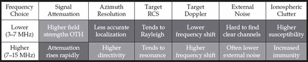
FIGURE 5.32 HFSW radar frequency selection requires striking a balance between reducing surface-wave attenuation (favored at lower frequencies) and all other competing factors listed above (favored at higher frequencies). © Commonwealth of Australia 2011.
For the purpose of simplifying the discussion, we may broadly consider HFSW radar operation in “low” and “high” frequency regimes denoted by 3–7 and 7–15 MHz, respectively. HFSW radars are usually not operated near the upper end of the HF band unless space-wave propagation to a line-of-sight target exists. We may also consider two nominal HFSW radar missions, namely, the detection of slow-moving high-RCS targets (i.e., large ships) at long ranges between 200 and 400 km, and the detection of fast-moving low-RCS targets (e.g., small aircraft) at short to intermediate ranges, defined as 50–100 and 100–200 km, respectively. We may also define a close range band of less than 50 km, noting that these are only indicative values.
The detection of fast-moving targets is often limited by background noise rather than clutter after Doppler processing. A possible exception occurs when spread-Doppler ionospheric clutter contaminates the range-azimuth cell containing the target. Ignoring this possibility for the moment, frequency selection for this target class essentially reduces to a tradeoff between three competing objectives: (1) surface-wave path-loss, (2) target RCS, and (3) background noise spectral density. For small (fighter-sized) aircraft, the target RCS tends to increase with frequency, but so too does the path-loss. At short to intermediate ranges, these two effects tend to roughly cancel each other out such that their product does not change dramatically on average in the “low” and “high” frequency regimes. However, the irreducible (spatially uncorrelated) component of the background noise spectral density tends to decrease at higher frequencies, particularly at night.
Moreover, it is usually less difficult to find clear frequency channels of the appropriate bandwidth at higher frequencies, particularly at night. Indeed, it is typically found that there are almost twice as many channels of a fixed bandwidth in 7–15 MHz as there are in 3–7 MHz. Ionospheric clutter is also less of a problem at higher frequencies on the NVI path. These considerations mean that it is often best to operate in the 7–15 MHz frequency regime to detect fast-moving low-RCS targets at short to intermediate ranges. Use of frequencies in the upper HF band leads to a significant increase in path loss at ranges beyond 50 km. At such ranges, the additional path loss is less likely to be canceled by an increase in target RCS. In summary, the “high” frequency regime is often considered to be more appropriate for the detection of fast-moving small-sized targets at short to intermediate ranges.
At close ranges, the surface-wave path-loss increases less rapidly with increasing frequency than it does at further ranges. At ranges less than a few tens of kilometers, increasing the frequency beyond 15 MHz is more likely to improve the net product between target RCS and path-loss, particularly for GFB targets that rise only a meter or so above the sea surface. Frequencies beyond 15 MHz may therefore be considered appropriate for the detection of small (low-flying) aircraft or GFB targets at close ranges.
On the other hand, operation in the “low” frequency regime (3–7 MHz) is necessary to keep path loss to within manageable limits at long ranges. Unfortunately, small targets fall well within the Rayleigh scattering region at such frequencies and their RCS drops precipitously. Many HFSW radar systems therefore find it difficult to reliably detect fast-moving small-sized targets at long ranges.
The RCS of large ships remains in the resonance region over the entire HF band so operation in the “high” frequency regime is unlikely to significantly increase the RCS for this target class. To optimize the detection of large ships at long ranges, the main option for increasing the received target echo power is to decrease the surface-wave path loss by operating in the “low” frequency regime (3–7 MHz). At low frequencies and long ranges, slow-moving targets are often detected against second-order sea clutter and potentially ionospheric clutter. Depending on sea-state, the power and Doppler spectrum extent of the second-order sea clutter tends to diminish as the operating frequency is lowered. On the other hand, in the “high” frequency regime (7–15 MHz), the surface-wave attenuation becomes prohibitively large at long ranges, especially for high sea-states. In this case, the path loss at long ranges can be large enough to submerge echoes from large ships and second-order sea-clutter below the background noise floor.
For these reasons, the “low” frequency regime is often considered more appropriate for the detection of large ships at long ranges. However, a major concern with operation below the maximum critical frequency of the E- or F-region is ionospheric clutter. This may at times justify the use of higher operating frequencies for the detection of large surface vessels at long ranges, particularly at night when spread-Doppler clutter may be received below the F2-layer critical frequency. Raising the operating frequency to reduce spread-Doppler clutter returned via the NVI path from the F2-layer comes at the expense of higher surface-wave attenuation and hence reduced detection range. During the day, when E-region ionization is well developed, dual-frequency operation may be used to combat the ionospheric clutter problem, as described in the next section.
An HFSW radar may at times be tasked to search for a specific type of target with known RCS characteristics. For example, the target of interest may be a certain type of fishing vessel such as the one considered in Trizna (1982). In this specific case, the target RCS for vertical polarization is dominated by a metal mast with a resonant frequency of 4.5 MHz. As shown in Trizna (1982), the target RCS may vary by as much as 10–15 dB across the “low” frequency regime 3−7 MHz. When a priori knowledge about the target RCS characteristics is available, the operating frequency may be tailored accordingly to maximize the power of the received echo. Clearly, the broad categorization of “low” and “high” frequency regimes is too coarse for frequency optimization in these specific cases.
5.5.2.2 Dual-Frequency Operation
Dual- or multi-frequency operation in HFSW radar differs from traditional frequency agility applied to interleaved dwells in the sense that the radar may contemporaneously rather than sequentially transmit and receive signals on different carrier frequencies. The data stream acquired in each frequency channel is processed independently (i.e., pulse compression, transient excision, Doppler processing, beamforming, CFAR, and peak detection). The waveform parameters set for each carrier frequency may be optimized for the detection and tracking of either ship or aircraft targets, but not both simultaneously. This is mainly due to the two types of target having very different velocities and detection update rate requirements for effective tracking.
When the waveform parameters on different frequencies are configured to detect the same target class (i.e., ships or aircraft), the peak detections resulting from the multiple processed data streams may be fed into a common tracker which associates them. The simultaneous detection of ships at one frequency and aircraft at another offers significant flexibility, but it does not yield the benefits of combining observations for the same targets illuminated at different frequencies. For simplicity, we restrict our attention to the use of only two frequencies (i.e., dual-frequency operation) for the detection and tracking of a single target class. The detection and tracking of ships is considered, as surface vessels often represent the primary target in HFSW radar.
The simultaneous use of two carrier frequencies can provide several advantages for HFSW radar (Leong and Wilson 2006). The first major advantage provided by dual-frequency operation is an improved capability to track ships through first- and second-order sea clutter. Due to the square-root relationship between the Bragg-line Doppler frequency and the radar carrier frequency, the relative separation between the target echo and nearest Bragg line in the Doppler spectrum is a function of carrier frequency. Provided the HFSW radar operates at two well-spaced carrier frequencies, a target echo masked by a powerful Bragg line at one carrier frequency (i.e., a blind speed) will be separated in Doppler frequency from the Bragg line at another carrier frequency.
Consider a practical example of a surface-vessel with a relative velocity of 9 m/s (17.5 knots). At a carrier frequency of 3 MHz, the target Doppler shift is 0.18 Hz for a monostatic radar configuration. The Doppler frequency of the nearest Bragg line is separated from that of the target echo by only 0.004 Hz in this case, which cannot be resolved with a CPI under 200 s. At a carrier frequency of 4 MHz, the target echo Doppler shift is 0.24 Hz, while the advancing Bragg line Doppler frequency is approximately 0.20 Hz. This increases the Doppler frequency separation by an order of magnitude to 0.04 Hz. A CPI of 100 s provides a classical Doppler frequency resolution of 0.01 Hz. For this CPI, the separation between the target echo and advancing Bragg line is equal to four FFT frequency bins at 4 MHz, but less than half a frequency bin at 3 MHz. Experimentally recorded HFSW radar data that illustrates this practical benefit of dual-frequency operation is shown in Figure 5.33.
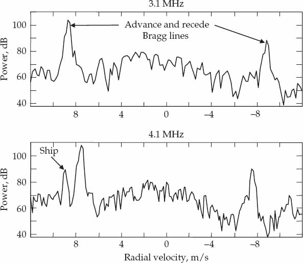
FIGURE 5.33 Target echoes from ships may not be detected when the Doppler frequency of the echo is close to that of a Bragg line. The top panel shows a situation where an echo from a ship target is masked by the advancing Bragg line at 3.1 MHz. Dual-frequency operation allow the target echo to be clearly distinguished from the advance Bragg line at 4.1 MHz (bottom panel). © Crown 2010. Government of Canada. (Courtesy of Dr. H. Leong, Defence R & D Canada.)
To summarize, echoes from a particular target received simultaneously by the same radar at two different carrier frequencies cannot both fall on a Bragg line in the Doppler spectrum. In an HFSW radar, the problem of Bragg-line masking can be addressed by dual-frequency operation provided the carrier frequency separation and CPI length are chosen appropriately. Specifically, the frequency separation and CPI length need to be such that the square-root versus linear Doppler frequency relationship can be resolved for the target relative velocities of interest.
In addition, the two frequencies should not be so far apart from the optimum frequency such that the target echo can be reliably detected in both frequency channels when not masked by a Bragg line. This enables an HFSW radar to detect ship echoes against second-order clutter plus noise regardless of the target relative velocity. A similar argument applies for target echoes masked by certain discrete second-order spectral components in the sea-clutter Doppler spectrum, which also follow a square-root relationship, similar to the Bragg lines.
A second advantage of dual-frequency operation is that it provides an alternative method for mitigating ionospheric clutter received on the NVI path. During the day, the approach is to select one operating frequency below the E-layer critical frequency and the other above it. The following discussion focuses on NVI ionospheric clutter because this path typically gives rise to the strongest returns and is often most problematic in terms of obscuring target echoes in the HFSW radar coverage.
Ionospheric clutter is returned by the E-layer at the lower operating frequency (which is typically set below 4 MHz at noon local time) and this reflection contaminates a band of range starting at around 100 km. The first affected range depends on the virtual reflection height of the NVI path, as well as the transmitter-receiver separation. Importantly, the E-layer prevents reflections from the higher altitude F-layer when operating below the E-layer critical frequency.
On the other hand, the signal at the higher frequency penetrates through the E-layer at near vertical incidence. This signal may be reflected back by the F-layer, resulting in clutter being observed beyond a distance of about 220 km. In principle, the lower and higher frequencies are affected by ionospheric clutter returned from the E-layer or F-layer, respectively, but not from both layers at the same time. Hence, a target echo at a given range will in principle be free of ionospheric clutter contamination in at least one of the frequency channels. Figure 5.34 shows a practical example of daytime ionospheric clutter received simultaneously by an HFSW radar at two different frequencies.

The mitigation of ionospheric clutter at night is more challenging because the D- and E-layers effectively disappear after sunset, but sufficient ionization to reflect HF signals remains in the F-region. At night, ionospheric clutter contamination from the F2-layer at ranges beyond about 200 km cannot be avoided by dual-frequency operation, unless one of the operating frequencies is higher than the F2-layer critical frequency. However, operation above the relatively high F2-layer critical frequency may not be a feasible option for HFSW radar due to the greater surface wave path-loss incurred. In other words, the use of higher frequencies attracts a considerable performance penalty for the detection of large ships at long ranges. Figure 5.35 illustrates the longer-range ionospheric clutter received from the F2-layer at night.
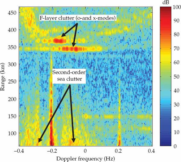
As shown previously, large surface vessels are found to have RCS values that exhibit significant aspect and frequency dependence in the lower HF band. At a given operating frequency, the target RCS will pass through (imperfect) nulls and enhancements as the aspect angle changes. Large ships may not be detected by an HFSW radar at aspect angles that fall in a deep RCS null. Importantly, RCS nulls may occur at quite different aspect angles when the operating frequency is changed by about 1 MHz near the low end of the HF band. This is evident in Figure 5.31, which shows the RCS variation of a large cargo freighter with aspect angle at 3.1 and 4.1 MHz based on NEC modeling (solid line) and the corroborating experimental measurements at 4.1 MHz (dotted line).
For target aspect angles near 28, 45, 62, 70, 75, 100, 105, 110, 130, and 150 degrees, it is observed from the modeling that the RCS passes through a relatively low value at one operating frequency and an enhancement at the other. Specifically, the predicted difference in RCS at operating frequencies of 3.1 and 4.1 MHz can be higher than 10 dB for certain aspect angles. Note that the deepest RCS nulls rarely line up at the same aspect angle at both frequencies. Simultaneous radar operation on two well spaced frequencies may therefore reduce the likelihood of missed target detections due to RCS nulls. Tracking ship targets through RCS nulls is considered to represent the third major advantage of dual-frequency operation. Another potential benefit is that relatively short-lived narrowband interference will only impact one frequency channel.
5.5.3 Example Systems
World-wide, perhaps a dozen or more countries have previous or currently active HFSW radar programs. This includes Canada, Unites States, Australia, Great Britain, Germany, France, China, Russia, Japan, and Turkey, for example. This section describes a selection of representative HFSW radar systems that have been designed and operated with surveillance applications as the primary mission. The performance of these systems against different target classes, as claimed in the literature, are also quoted to provide an indication of nominal capabilities. The HFSW radars discussed in more detail are the two-site Iluka and SECAR systems, developed in Australia, the single-site SWR-503 system, developed in Canada, and the truly monostatic BAE surface-wave radar, developed in the United Kingdom.
For the reader interested in delving further, information on several other former and present HFSW radar systems may be found in a number of excellent articles. For example, the HFSW radar demonstrator in Biscay Bay, France, developed by ONERA and the French MOD (DGA) is described in Menelle et al. (2008), the Wellen Radar (WERA) system originally developed by the University of Hamburg, Germany, is described in Dzvonkovskaya et al. (2008) and references therein, while progress in HFSW radar activities in China have been reported in Liu, Xu, and Zhang (2003) and (Liu 1996).
5.5.3.1 Iluka and SECAR Systems
Research and development in HFSW radar by the Australian government started in 1993 when an experimental system was designed and deployed by the Defence Science and Technology Organisation (DSTO) at a site north of Adelaide, South Australia (Anderson, Bates, and Tyler, 1999). Following the successful trials of this experimental system, a much larger and more capable radar named Iluka was designed, built, and installed near Darwin in northern Australia. Several different organizations were involved in the Iluka project, including DSTO, Telstra Applied Technologies (TAT), and the Centre for Sensor Signal and Information Processing (CSSIP).
A series of scientific experiments were conducted using the Iluka system in 1998. TAT later sublicensed its HFSW radar interests to Daronmont Technologies (DarT), which developed a production version of the radar named Surface-wave Extended Coastal Area Radar (SECAR). In conjunction with scientists and engineers from DSTO and CSSIP, DarT conducted extensive trials with SECAR in 2000 from a receive site on Bathurst Island, north of Darwin. The Iluka and SECAR systems are not currently deployed in an operational role, but both systems represent examples of bistatic HFSW radars designed for the surveillance of air and surface targets within the EEZ.
The Iluka HFSW radar was designed to operate in the 5–15 MHz frequency range, although capable of operating at higher frequencies if needed. This system consisted of a primary high-power transmit site, located at Stingray Head (65 km south-west of Darwin), and a secondary low-power transmit site at Lee Point (10 km north-east of Darwin). The receive site, located at Gunn Point (30 km north-east of Darwin) was separated by about 95 km from the high-power site, and approximately 18 km from the low-power site. The secondary low-power site was mainly used to investigate the dependence of sea clutter characteristics on illumination geometry.
The receiver site was sufficiently isolated from both transmitters to allow operation with unit duty-cycle frequency modulated continuous waveforms (FMCW). The Iluka receiving system was based on a 500 m long ULA of 32 vertical monopoles, each connected to a well-calibrated HF receiver with boresight oriented in a westerly direction (at right-angles to the shoreline). At the low-power site, a 250-W amplifier drove a pair of monopoles spaced 20-m apart and fed in anti-phase. A single log-periodic dipole array (LDPA) antenna connected to 10-kW transmitter was used at the high-power site. This radar routinely detected 42 m patrol boats at ranges beyond 150 km, and small low-flying aircraft 20-m above sea surface at ranges in excess of 200 km. Due to the accompanying space-wave propagation, commercial aircraft at high altitudes could be detected at much greater distances.
The architectural characteristics of the SECAR radar are summarized in Table 5.3, while Figure 5.36 shows pictures of the SECAR transmit antenna and receiver array. A comprehensive description of the SECAR system can be found in (Anderson et al. 2003). The SECAR system has demonstrated detection performance of large surface vessels, such as Frigates and offshore trawlers out to the EEZ limit (370 km). Smaller fishing boats and GFBs have been detected up to ranges of 120 km and 70 km, respectively, while low-flying fighter-sized aircraft may be detected to ranges in excess of 200 km. A salient advantage of the FMCW bistatic HFSW radar configuration is that targets such as GFBs can be detected effectively at close (and long) range (a few tens of kilometers). This can be problematic for single-site or truly monostatic HFSW radar systems that use pulse waveforms due to the significant eclipsing loss experienced at close and long ranges as a result of the finite pulse duration.

TABLE 5.3 Nominal architecture and operating parameters of the SECAR HFSW radar system.
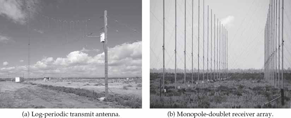
FIGURE 5.36 The SECAR HFSW radar transmit antenna is single vertical log-periodic dipole array (LDPA), while the receive antenna is a uniform linear array of twin-monopole elements configured to provide front-to-back directivity. © Commonwealth of Australia 2011.
5.5.3.2 SWR-503
Raytheon Canada System Limited (RCSL) and the Canadian Department of National Defence (DND) developed two single-site HFSW radars which commenced operation off the east coast of Newfoundland at Cape Race and Cape Bonavista in 1999. These two radars, designated SWR-503, are separated by 226 km approximately on the longitudinal line 53° W to provide overlapped coverage of an area in the Grand Banks. The operating frequency range is nominally between 3 and 5 MHz, which is best suited to the detection of medium to large surface vessels at intermediate to long distances as the primary mission. The detection and tracking of small private aircraft and GFBs is more challenging at these low frequencies due to the significantly lower RCS of such targets plus the need to use short CPIs for effective Doppler processing and rapid detection updates.
Detailed descriptions of SWR-503 can be found in Ponsford, Sevgi, and Chan (2001), as well as in Leong (2002) and Leong, Helleur, and Rey (2002). The key operational parameters of the SWR-503, as quoted in these references, are listed in Table 5.4. The HFSW radar at Cape Race employs a log-periodic transmit antenna and a ULA receive antenna composed of 16 doublet elements. The receiving doublets, each consisting of two kite-shaped monopoles, are phased end-fire and the separation between adjacent doublets is 33.33 m. The doublet elements are spaced half-wavelength apart at the radar design frequency of 4.5 MHz. The electronically steered receive beams have a main lobe width of approximately 9 degrees, but azimuth estimates typically have an error of less than 1 degree for well-resolved radar echoes. The coverage arc is ±60 degrees from boresight. The HFSW radar at Cape Bonavista is very similar to the Cape Race system, except a that quadlet is used as the receive antenna element instead of a doublet.

TABLE 5.4 Nominal design parameters of the HFSW radar at Cape Race (46:39:07 N, 53:05:24 W), Newfoundland, Canada. The boresight of the receiving array is 121 degrees clockwise from true north.
The transmitter generated an average power of 1.6 kW, and sea clutter was typically found to be the limiting disturbance to ranges greater than 350 km during the day (using CPIs of hundreds of seconds). However, at night the radar is usually externally noise limited beyond approximately 150 km. The system could employ an 8-bit complementary phase-coded sequence on transmit, which permits range sidelobe reduction and high pulse repetition frequency (PRF) operation through the suppression of range-wrapped ionospheric clutter. For example, a phased-coded pulse may have a length of 400 microseconds with a bit duration of 50 microseconds (Leong 2002). The radar could also use “mismatched” phase-code sequences to enable the suppression of strong narrowband co-channel interference signals (Ponsford, Dizaji, and McKerracher 2003).
The nominal operating bandwidth of 20 kHz provides a group-range resolution of 7.5 km, while oversampling with a period of 10 microseconds can yield a measurement accuracy of about 0.3 km for well-resolved radar echoes. The cross-range resolution is roughly equal to 50 km at the 200 nmi (370 km) EEZ limit. CPIs of 10 seconds (air mode), 100 seconds (ship mode), and 1000 seconds (stationary targets) have been used to provide relative velocity resolutions of approximately 5, 0.5, and 0.05 m/s, respectively, at 3 MHz. Extensive trials have been conducted to demonstrate beyond the horizon detection of aircraft to 300 km, surface targets to 500 km, and icebergs to 300 km. Medium sized ships such as the Ville de Quebec (length 436 ft, height 140 ft) were tracked to ranges of up to 235 km, while smaller vessels such as the Anne S. Pierce (length 117 ft, height 55 ft) and Artic Pride (length 64 ft, height 45 ft) were tracked to approximately 110 km (Leong, Helleur, and Rey 2002).
5.5.3.3 BAE SWR System
The HFSW radar system developed by BAE systems in the United Kingdom is described in the two-part paper of Dickel, Emery, and Money (2007). Its predecessor version was described by Emery, Money, and Matthewson (2004). The first distinguishing feature of this system is that it uses a single uniform linear array (ULA) of antenna elements for transmission and reception. This truly monostatic HFSW radar has the advantage of a relatively small real-estate footprint by dispensing with the need for a separate transmit antenna or a second radar site. A truly monostatic or single-site system is not subject to variations in performance caused by the changing bistatic angle to different points in the coverage. A picture of the BAE HFSW radar array is shown in Figure 5.37.

FIGURE 5.37 Uniform linear array of 16 (doublet pair) tetrahedral dipole antenna elements used in the BAE surface-wave radar. The middle six elements are fitted with high-power duplexers and used as reciprocal antennas for transmission and reception.
The ULA is typically composed of 16 identical antenna elements, each configured as a doublet pair of tetrahedral dipoles phased in the endfire direction with approximately 15 dB front-to-back ratio (Boswell, Emery, and Bedford 2006). All antennas in the array are used for reception, while the middle six antennas are connected to a bank of solid-state high-power duplexers, which enable transmission and reception using the same (i.e., reciprocal) elements. The smaller transmit aperture provides a relatively broad beam in azimuth, similar to that provided by a single LPDA antenna. Besides requiring less real estate than an LPDA antenna, using an array of rigid transmit antennas tends to reduce Aeolian noise (phase noise) caused by movement of radiating elements under wind stress. It also allows the transmit beam to be digitally steered and shaped. However, these benefits may come at the expense of reduced frequency range with respect to an LPDA, as compact elements typically exhibit broadband performance over an octave.
The six tetrahedral dipole antenna elements in the middle region of array are driven by individual digital waveform generators connected to 1-kW solid-state power amplifiers. The waveform generators are fully programmable to simultaneously transmit different waveforms in a multiple-input multiple-output (MIMO) architecture. For example, the system can be programmed to synthesize a simple pulse, linear or nonlinear chirps, and stepped frequency signals up to a maximum bandwidth of 30 kHz.
The ability of the middle six antenna elements to independently transmit different radar waveforms at different carrier frequencies represents another distinguishing feature of this system. A digital waveform generator per element allows the transmit resource to be divided among multiple frequencies without degrading performance in a clutter-limited environment (i.e., low-power floodlight illumination using a subset of the six transmit elements at each frequency). A “spotlight” mode that involves electronic steering of narrow transmit beams with higher gain using all six radiating elements may be used in noise-limited conditions.
As described in Dickel, Emery, and Money (2007), a doublet at one end of the array is configured with an inverse pattern to serve as a Rear Lobe Blanking (RLB) antenna, while a doublet at the other end of the array is used for environmental monitoring as well as beamforming. The use of wide-band receivers that sample the signal at the RF element level allows for digital down conversion and processing of up to four simultaneous frequency channels per element. Signal and data processing up to the plot extraction stage are run in parallel for each of the four down converted channels. Different processing steps/parameters may be used in each channel to contemporaneously perform air and surface target surveillance, for example. The peak data resulting from each of the four channels is then fused to produce target tracks in the final processing stage.
The simultaneous use of up to four distinct carrier frequencies, combined with plot level fusion of the processed outputs from different frequency channels provides a higher level of immunity to incidental man-made interference, target RCS fades, and Bragg-line masking. Multi-frequency operation also provides greater scope to optimize frequency selection for different target classes, ranges, and speeds under the prevailing environmental conditions. The BAE HFSW radar has nominal a frequency range of 8–16 MHz and can provide coverage across a 110 degree sector. Surface vessels may be tracked to ranges of 220 km over an area of approximately 30,000 square kilometers, while aircraft may be tracked simultaneously out to 350 km (large commercial airliners) over a coverage twice the size.
Aircraft target localization accuracy is approximately 1 km in range and 0.5 degrees in azimuth relative to air traffic control (ATC) radar acquisitions Dickel, Emery, and Money (2007). In Emery, Money, and Matthewson (2004), the rms position error for a ferry ship tracked by HFSW radar were measured at 1.3 km in range and 0.7 degrees in azimuth relative to known GPS ground-truth information. This accuracy is considered good for a long-range sensor with inherently “coarse” spatial resolution. Target echoes become partially eclipsed by the transmit pulse duration at close ranges, and degradation in detection performance is experienced. SNR degradations due to eclipsing loss become significant below about 20 km (Emery, Money, and Matthewson 2004), which represents the nominal minimum range of the system.
____________________
1 For example, the RISP gain is 1.5 for a vertical Hertzian dipole on a PEC plane, and 1.64 for a vertical λ/4 monopole on a PEC plane. Further discussion on the use of RISP gains in preference to dBi values can be found in Milsom (1997).
2 Using the antenna gain definitions in Eqn. (5.3),  has a value of approximately −32 dB for a fully developed sea and a semi-isotropic angular spreading function when ωd falls on a Bragg line Doppler frequency. Depending the form of σ2(ω), the value of may be 20–40 dB (or more) below the first-order contribution at Doppler frequencies that place the target echo in the second-order clutter continuum for a CPI of T = 100 s.
3 Reciprocal antennas have been used in an HFSW radar system to be described in Section 5.5.
..................Content has been hidden....................
You can't read the all page of ebook, please click here login for view all page.