
CHAPTER 11
Space-Time Adaptive Processing
Space-time adaptive processing (STAP) refers to a class of multi-dimensional adaptive filtering techniques which are used in radar to simultaneously combine data received across the elements of an antenna array with samples acquired in the dimensions of slow- and/or fast-time over a coherent processing interval to produce a filtered scalar output. The primary goal of the STAP filter is to maximize the output signal-to-disturbance ratio (SDR) by suppressing clutter and interference in each processed azimuth-range-Doppler cell. In the presence of powerful disturbance signals, STAP can significantly improve the target detection performance of a radar system with respect to conventional processing.
STAP is a topic which has received enormous attention in the literature. The intense interest over the last two decades in particular has led to the development of a wide variety of STAP techniques for different radar systems, practical applications, and operational scenarios. The scope of this chapter is not to review the extensive collection of theoretical and experimental works on STAP, but rather to focus on the specific STAP implementations that hold most promise for OTH radar systems.
For a general introduction to the subject of STAP, the reader is referred to a number of authoritative treatments, such as the definitive texts by Klemm (2002) and Guerci (2003), and the comprehensive review articles of Melvin (2004), Wicks, Rangaswamy, Adve, and Hale (2006), and references therein. The technical report by Ward (1994) and seminal paper of Brennan and Reed (1973) are also highly recommended.
In certain situations of practical interest to radar operators, STAP offers the potential for more effective disturbance cancelation than separate spatial and temporal adaptive processing. Depending on the configuration employed, STAP can involve the use of antenna elements or beams as spatial channels, and either time or frequency domain samples in each spatial channel. Restricting attention to antenna-element and time-domain architectures, STAP implementations may incorporate slow-time and/or fast-time samples to combat disturbances such as clutter and/or interference, which inherently possess different correlation properties.
Areas in which STAP offers significant benefits relative to sequential or “factored” space-time processing include the rejection of backscattered surface clutter for radars mounted on moving platforms (slow-time STAP), and the rejection of diffusely scattered multipath interference, which may be received through the main lobe of the antenna pattern (fast-time STAP). The most general “fully adaptive” STAP approach simultaneously combines signals from antenna elements, slow-time samples, and fast-time samples (3D-STAP). This architecture has been proposed for the problem of jointly mitigating surface clutter and terrain-scattered interference in airborne radar (Fante and Torres 1995).
Important practical issues for STAP include the need for sufficient and statistically homogeneous training data, as well as low computational load for real-time processing. Such considerations have led to a taxonomy of partially adaptive algorithms with reduced dimension or rank (Goldstein and Reed 1997). Self-configuring STAP techniques that are robust to instrumental imperfections and changing environmental conditions (without requiring operator intervention) are also highly desirable in practice.
The first section of this chapter describes three different STAP architectures implemented in the antenna-element/time domain and discusses the motivation for each architecture in connection with the characteristics of the disturbance to be mitigated. The main purpose of this section is to identify the STAP typologies that are most suitable for OTH radar, and to delineate the peculiarities of the STAP problem for OTH radar with respect to that encountered in airborne microwave radar systems.
Data models are formulated in the second section to describe the characteristics of surface-scattered clutter and diffuse multipath interference signals received by OTH radar after reflection from the ionosphere. The third section presents standard and alternative STAP techniques to address the problem of rejecting non-stationary diffuse multipath interference or “hot clutter” in OTH radar. The performance of these algorithms is illustrated using simulated data based on the formulated data models.
The final section describes a post-Doppler STAP technique for canceling a mixture of narrowband interference and spread-Doppler clutter that is statistically heterogeneous in range. With practical applications in mind, this method incorporates a reduced dimension beam-space architecture to ease demands on sample support and computational load. An important theme relevant to the entire discussion is that the added sophistication and computational complexity of STAP algorithms needs to be justified in terms of the practical performance benefits relative to processing schemes that operate separately on a single radar data-cube dimension at a time.
11.1 STAP Architectures
To explain and motivate the different antenna-element/time-domain STAP architectures, it is useful to recall the “anatomy” of the radar data cube. The radar system operates by collecting data over a coherent processing interval (CPI), which consists of P transmitted pulses or “sweeps” emitted at a pulse repetition frequency of fp pulses per second. The receiving system is composed of N spatial channels, consisting of antenna elements or sub-arrays, for example, with each reception channel being connected to an individual digital receiver.
After down-conversion and filtering, the received in-phase and quadrature (I/Q) components of the baseband signal are sampled at the Nyquist rate of ft samples per second, such that K complex samples are acquired in each pulse repetition interval (PRI). The raw data cube collected in this manner over a single CPI therefore consists of N × P × K complex samples. Increments acquired at the Nyquist rate within a particular PRI are referred to as “fast-time” samples or range bins, while those resulting across different PRI intervals over the CPI are termed “slow-time” samples (Griffiths 1996).
This section is divided into three parts, which describe the main characteristics of slow-time, fast-time, and fully adaptive 3D-STAP. These different STAP techniques are described with a view to explaining the potential application of each to OTH radar. Figure 11.1 summarizes the filter dimensions and input/output data formats of the three STAP typologies considered, along with representative applications, which will be described in more detail below.
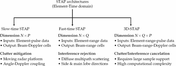
FIGURE 11.1 Different STAP architectures for processing in the antenna-element/time domain with a representative application in each case. The number of fast-time samples used is generally less than the maximum number available, i.e., Q < K.
11.1.1 Slow-Time STAP
Slow-time STAP operates on a single range cell in turn and produces an output that is a weighted linear combination of spatial samples collected by different antenna elements in the array, and temporal samples acquired over multiple coherent pulses of the radar waveform during the CPI. The filter dimension corresponding to the full slow-time STAP architecture is therefore N × P. At a given range cell, the STAP weights are adjusted to provide an output for each combination of beam steer direction and echo Doppler frequency at which targets are sought. Ideally, the STAP weights are synthesized in a manner that maximizes the signal-to-disturbance ratio in the output beam-range-Doppler cells. Here, useful signals refer to target echoes matched to the interrogated steer direction and Doppler frequency, while disturbance refers to both clutter and interference in general.
When it is necessary to reduce the number of degrees of freedom (DOFs) in the STAP processor, partially adaptive slow-time STAP configurations may be implemented post-Doppler or in beam space, for example. Alternatively, more sophisticated rank-reduction transforms based on singular-value decomposition may be used. In any case, slow-time STAP techniques operate on all or part of the information contained in the receivers and pulses of the radar data cube. For the time being, we shall not distinguish between full and partially adaptive slow-time STAP, or concern ourselves with issues regarding training data and computational load. These aspects are of course very important for practical implementation, but peripheral in the sense of identifying the main objective of the processor itself.
The slow-time STAP approach has received considerable attention in the context of its application to airborne microwave radar systems. The question arises as to the driving factors which motivate this two-dimensional processing architecture for such systems, and the conditions in which slow-time STAP may be expected to provide performance benefits relative to the application of beamforming and Doppler processing separately.
For the case of a moving radar platform, a large part of the answer resides in the strong coupling that exists between the direction of arrival and Doppler frequency of radar signals backscattered from extended regions of the Earth’s surface. More specifically, relatively faint target echoes received in the main beam can be masked by strong surface clutter returns that share the same Doppler frequency and group range (either coincident or ambiguous) as the target echo, but are incident from directions other than the radar look direction.
An important objective of slow-time STAP in airborne radar systems is to mitigate sidelobe clutter, which is distributed in Doppler frequency due to platform motion. It is often difficult for a conventional beamformer to achieve extremely low sidelobes in practice due to array calibration uncertainties and local scattering effects arising from the presence of the aircraft. In addition, conventional processing typically achieves relatively low sidelobes at the expense of an increase in main-lobe width. As adaptive beamforming may alleviate some of these issues, it is reasonable to ask why slow-time STAP is applied in preference to the combination of adaptive beamforming and Doppler processing.
The main advantage of slow-time STAP with respect to adaptive beamforming stems from the fact that the surface clutter is incident from a continuum of directions and therefore tends to have full spatial rank. This makes clutter rejection via pure spatial processing ineffective in general. However, due to the strong DOA-Doppler coupling of the backscattered clutter, the energy contained in such signals has the potential to be concentrated in a relatively low dimensional subspace of the space-time covariance matrix formed in the joint antenna-element/slow-time domain. This property opens up the possibility for more effective sidelobe-clutter rejection using slow-time STAP.
Slow-time STAP provides the possibility to simultaneously cancel a limited number of jamming sources that may occupy all range-Doppler bins (i.e., broadband interference), but are not incident from the same direction as the target echo (i.e., not entering through the main beam). For an airborne radar system, this typically includes the direct and specularly reflected interference paths but not diffusely scattered components incident from the main beam direction. The advantage of slow-time STAP over adaptive beamforming when sidelobe interference is present is that such interference can in principle be rejected effectively even when clutter-free training data is not available.
OTH radars operate with fixed land-based receive and transmit systems; an exception to this is HF surface-wave radars installed on moving ship-borne platforms, but this case will not be considered further. In general, backscattered surface clutter received by OTH radars exhibits relatively weak (if any) ionospherically-induced DOA-Doppler coupling.1 In a given range cell, both main-lobe and sidelobe clutter backscattered from the OTH radar transmitter footprint often occupy a similar Doppler frequency band typically near 0-Hz. In other words, target echoes are often Doppler-shifted by a similar amount relative to both the main-lobe and sidelobe clutter in OTH radar. In this situation, slow-time STAP provides minimal or no advantages with respect to factored space-time processing.
As standard Doppler processing is often quite effective for separating moving target echoes and quasi-stationary surface-clutter returns (incident from all directions) into different Doppler bins, there is often no strong motivation to apply slow-time STAP in OTH radar systems. A possible reason to justify the additional computational complexity of slow-time STAP relative to the application of adaptive beamforming and Doppler processing is when supervised training data containing only interference and noise contributions is difficult to obtain. Clutter contamination in the training data used for adaptive beamforming can bias the weight estimates and degrade interference-plus-noise rejection performance. Since there are different methods for obtaining such training data in practice, slow-time STAP has not found widespread use in OTH radar systems.
11.1.2 Fast-Time STAP
The schematic diagram in Figure 11.2 illustrates the fast-time STAP architecture which operates on data from a single radar pulse in turn. Here, the output is a weighted linear combination of spatial samples acquired by the receiving elements of the antenna array and multiple fast-time samples corresponding to different range-gates in a PRI. Note that the fast-time samples are delayed by Ts = 1/fs seconds, where for a receiver bandwidth B, the time-bandwidth product is typically less than or equal to unity BTs ≤ 1.

FIGURE 11.2 The fast-time STAP architecture implemented in the element-time domain combines data from N antenna sensors and Q fast-time samples.
The dimensionality of the full fast-time STAP architecture would be N × K, which can be large when many range cells are processed. To train such a filter in practice, only a small subset of range taps Q  K are used such that the filter dimension is reduced to N × Q. The fast-time STAP weights are ideally adjusted to maximize the output SDR for each beam steer direction and range bin processed. In this sense, fast-time STAP may be viewed as an extension of adaptive beamforming, since the output samples correspond to beam-range-pulse data.
Unlike slow-time STAP which generates beam-Doppler outputs for each range cell processed, the fast-time STAP outputs are in the PRI domain and must be subsequently Doppler processed to coherently integrate the pulses in the CPI. For additional information pertaining to the fast-time STAP architecture, the reader is reffered to Fante and Torres (1995), Kogon, Williams, and Holder (1998), Jouny and Culpepper (1995), and Griffiths (1997) and references therein.
The disturbance type which motivates the fast-time STAP architecture in airborne radar systems is known as terrain-scattered jamming (TSJ) or “hot clutter.” A jamming signal is generally not received as a simple rank-one spatial interferer incident on the sidelobes of the antenna radiation pattern. This would require the transmit antenna of the jammer to have a fictitious (unrealistic) “pencil beam” with no sidelobes such that only the “direct-path” interference is received by the radar. Real antennas have sidelobes, and consequently, significant amounts of jammer energy may be scattered from the Earth’s surface into the radar, resulting in both in-plane and out-of-plane multipath interference.
Since terrain and sea surfaces are never perfectly smooth, the jamming signal is not specularly reflected but rather diffusely scattered, possibly over an extended area that spans a wide angular region. As a result, high levels of jammer energy can enter through both the mainbeam and sidelobes of the receive antenna pattern. In general, spatial-only adaptive processing (SAP) does not provide a solution for the hot-clutter problem, since this type of interference cannot be canceled effectively by simply placing “nulls” in the receive antenna pattern alone.
A consequence of diffuse multipath scattering is that the total number of interference paths summed over the number of independent sources can significantly exceed the number of spatial DOF available (i.e., the number of antenna elements N). In other words, the effective number of linearly independent interference components to be canceled may overwhelm the processor in the sense that the resulting interference spatial covariance matrix is of full rank N. Moreover, while the direct and specularly reflected jammer paths may be received from sidelobe directions, diffusely scattered multipath components can potentially enter through the main beam, particularly when scattering is from rough surfaces that act to spatially distribute the signal over a broad continuum of angles. The presence of main beam interference poses a problem for SAP even when the interference spatial covariance matrix has low rank.
Adaptive beamforming cannot be expected to effectively mitigate the composite hot-clutter signal when the condition of full rank or main-beam interference arises. Jamming signals are often assumed to emit waveforms that are uncorrelated with that of the radar and to have a bandwidth that is comparable with the receiver bandwidth. It follows that temporal DOF available in the slow-time STAP architecture cannot be used to mitigate such signals due to the long interval between pulses relative to the jammer waveform correlation time. However, the hot-clutter multipath components may be highly correlated with each other over time intervals in the order of the inverse of the system bandwidth. Thus, a STAP architecture that exploits fast-time taps can be effective for removing hot clutter.
The primary goal of fast-time STAP in airborne radar systems is therefore not to cancel the backscattered clutter signal, but rather to mitigate diffuse multipath interference received in the main beam and sidelobes of the antenna pattern. During the relatively short PRI, hot clutter from a particular source may be described as a linear combination of complex weighted and delayed replicas of the source waveform. In the fast-time STAP architecture, the finite impulse response (FIR) tap-delay-line filter behind each antenna element can in principle reverse the TSJ formation process. System identification requires the length of the FIR filter to be commensurate with the maximum impulse response duration of the propagation channel for the case of a single source. As we shall see later, the rejection of hot clutter from one or more sources may be achieved with less restrictive conditions on the number of required fast-time taps.
A key point is that the time dispersion of the hot-clutter channel needs to be acquired by each fast-time delay line at a temporal resolution that ensures the interference is not undersampled, i.e., BTs < 1 (Fante and Torres 1995). Essentially, the idea behind this architecture is that interference components received from scatterers located in the direction of the main beam may be canceled using multipath versions of the same signal received from highly correlated scatterers of the same source that are located outside the main beam but which are simultaneously captured within the fast-time tap-delay lines. This fast-time STAP concept will be described in more detail later.
The use of fast-time STAP for OTH radar applications was investigated in Anderson, Abramovich, and Fabrizio (1997), Abramovich, Anderson, Gorokhov, and Spencer (1998), and Abramovich, Anderson, and Spencer (2000). In this application, the different ionospheric layers which reflect the HF interference signal are responsible for creating the “diffuse multipath” phenomenon. The various ionospheric layers may be regarded as irregular reflection surfaces that diffusely scatter the interference signal from source to receiver along multiple propagation paths. In addition, the constant electron-density contours defining these scattering surfaces do not maintain a rigid structure over the relatively long (OTH radar) CPI. For example, the received interference modes are typically Doppler-shifted due to the mean or regular component of ionospheric layer motion. Importantly, any differential Doppler shift between these modes causes the hot-clutter channel, and hence the optimum fast-time STAP filter, to become time dependent over the CPI.
If the propagation paths involve reflections from highly perturbed ionospheric regions, such as those often encountered at low and high magnetic latitudes, significant random fluctuations of the channel can also contribute to the “non-stationarity” of the interference space/fast-time covariance matrix over the CPI. This motivates the use of fast-time STAP in OTH radar with the filter weights being updated a number of times within the CPI to counter non-stationary multipath interference.
A large portion of this chapter is devoted to the description of time-varying fast-time STAP algorithms that can effectively deal with this practical problem. An analogous effect may be observed in airborne radar systems due to the relative motion between the radar platform and jamming source(s). However, the airborne radar case differs in some important respects, and only algorithms appropriate for OTH radar applications will be discussed in this chapter.
11.1.3 3D-STAP
The most general “fully adaptive” STAP operates simultaneously on all three data-cube dimensions of elements, ranges, and pulses. Figure 11.3 illustrates this processor which was motivated and analyzed for the case of airborne radar systems in Fante and Vacarro (1998), Rabideau (2000), and Seliktar, Williams, and Holder (2000), for example. This type of approach can in theory solve the problem of joint hot- and cold-clutter suppression, where the latter refers to ordinary backscattered radar signal clutter. To jointly mitigate hot and cold clutter, both fast-time and slow-time temporal DOF are needed in addition to spatial DOFs. Simultaneous processing of all three data-cube dimensions is also called 3D STAP in the radar nomenclature. However, it is rarely possible to effectively implement the full 3D-STAP architecture in practice due to problems associated with the large processor dimension. In the 3D-STAP processor, the number of adaptive DOFs grows to N × Q × P, where Q is the number of fast-time samples or range bins used in the tap delay-line. For OTH radar systems with typical parameters of N = 32 and P = 128, this results in a prohibitively large weight-vector dimension of N × Q × P = 16384 for Q = 4 fast-time taps. The major concern for STAP architectures with many adaptive degrees of freedom is the lack of statistically homogeneous training data to effectively estimate the adaptive filter coefficients. Another important issue is the high computational load associated with computing the fully adaptive STAP solution. In airborne moving target indicator (MTI) applications, the relatively low-system dimensions (e.g., P ≤ 3 and N ≤ 16) may allow 3D-STAP to be implemented effectively (Abramovich et al. 1998).

FIGURE 11.3 The general fully adaptive STAP architecture implemented in the element-time domain combines data from N antenna sensors, Q fast-time samples (range bins), and P slow-time samples (coherent pulses). The tap delays are such that BTs < 1 where Ts Tp = 1/fp.
Rank-reduction transforms such as those proposed by Guerci, Goldstein, and Reed (2000) may be used to reduce the number of adaptive DOF. A rank-reduced 3D STAP could be proposed for OTH radar, but the underlying basis for such an approach would be poorly motivated for two reasons. First, ordinary clutter does not often exhibit significant angle-Doppler coupling in OTH radar, so the combination of space / slow-time processing is unlikely to provide significant cold-clutter mitigation benefits relative to standard Doppler processing. Second, the cold-clutter is usually received via relatively stable ionospheric propagation paths, which are often optimized by the choice of operating frequency, but the hot clutter typically originates from sources that are arbitrarily located with respect to the surveillance region, and may therefore propagate to the radar via reflections from highly perturbed ionospheric regions. This gives rise to a situation where the hot-clutter statistical properties are non-stationary over the CPI and time-dependent adaptation of the STAP filter is required for effective mitigation, while those of the cold clutter may be relatively stationary and not require the adaptive filter to be updated during the CPI.
The joint removal of hot and cold clutter is often not considered for OTH radar. One possible exception is for cases where hot-clutter-only training data cannot be obtained due to the presence of cold-clutter in all available ranges. This particular situation, which motivates 3D STAP in OTH radar, will not be considered here but has been treated in Abramovich, Anderson, and Spencer (2000). In summary, the fast-time STAP category represents the most well-motivated candidate out of all STAP architectures for practical application in OTH radar. For this reason, this chapter focuses on STAP techniques within this class.
11.2 Data Model
OTH radar systems are required to operate in signal environments where the composite disturbance is generally the sum of surface-scattered clutter, diffuse multipath interference (from one or more sources), and additive noise, all of which compete for detection against relatively faint target echoes. This section describes models for the various signal components received by an OTH radar in all three data-cube dimensions. Relatively simple models are described for the target and additive noise, while more detailed attention is paid to modeling the surface clutter and diffuse multipath interference, which are the dominant components to be mitigated in the received signal.
An important aspect of the formulated data models is that they allow realizations of OTH radar data to be readily generated for evaluating signal processing performance in computer simulations. The simulation results showing the performance of various fast-time STAP algorithms in Section 11.3.3 are based on synthetic data generated using the data model presented in this section.
11.2.1 Composite Signal
Let xk (t) ∈ CN be the N-variate spatial snapshot vector received by an array of N antenna sensors at fast-time sample k = 1, …, K and slow-time sample t = 1, …, P within the CPI. In general, xk(t) may be written as in Eqn. (11.1), where ck(t) is ordinary radar clutter backscattered from the Earth’s surface (cold clutter), jk (t) is the superposition of diffusely scattered multipath interference components from all jamming sources (hot clutter), and nk(t) is the sum of internal and external additive noise from other sources. The potential presence of a point-target echo is represented by the term sk(t), which is the useful signal.
(11.1)
For a uniform linear array (ULA) steered to a cone angle-of-arrival ϕ0, a useful signal incident from the radar look direction may be expressed in the form of Eqn. (11.2). Here, a is a complex scalar amplitude, ψk is the signal waveform, fd is the target Doppler-shift normalized by the PRF, s(ϕ0) is the steering vector on the ULA manifold, and γk is a range-dependent phase. A more complex model incorporating spatial spreading and temporal fading could be proposed, while other practical issues such as range straddling and range sidelobes could also be accounted for. Similarly, it would be possible to model mismatches in useful signal DOA, or extend the model to 2D arrays steered independently in azimuth θ0 and elevation φ0. However, such generalizations detract from the main intent of describing the key points, so the simplest target model in Eqn. (11.2) may be adopted for this purpose. For example, a signal matched to range bin k0 has a fast-time signature ψk = δ(k − k0) for a pulsed-waveform (PW) system, whereas for a continuous-wave (CW) system, ψk = up(k − k0), where up(k) is the transmitted signal pulse. It is convenient to consider the former case as it enables us to directly interpret fast-time samples as range bins. However, the main concepts illustrated in the following discussion are equally applicable to CW systems, as explained later.
(11.2)
The additive noise nk(t) is in general a mixture of internal receiver noise (i.e., thermal noise) and naturally occuring external noise (i.e., ambient noise). For the purpose of the following analysis, we avoid delving into the fine detail of physical noise models and simply assume that this process is complex circular Gaussian distributed and white across all radar data-cube dimensions. In other words, the additive noise has spatial and temporal correlation properties given by Eqn. (11.3), where  is the noise power per antenna element, and IN is the N-dimensional identity matrix. In Eqn. (11.3), E{·} denotes statistical expectation, † is the Hermitian (conjugate transpose) operator, and δkk′ is shorthand notation for the delta function δ(k − k′). As the cold- and hot-clutter disturbances are much more powerful than the additive noise, the structure or “color” of the additive noise is largely inconsequential because nk(t) is not the signal contribution that limits performance when hot clutter is present.
(11.3)
The fast-time STAP architecture considered here jointly operates on data acquired by the N antenna sensors of the array (i.e., element-space) and Q successive fast-time samples or range bins. Recall that Q is the number of fast-time taps in the delay line for each antenna sensor. The collection of these complex samples are conveniently assembled into the NQ-variate “stacked” data vector  defined in Eqn. (11.4). The stacked vectors for the useful signal
  , cold clutter
  , hot clutter
  , and additive noise ñk(t) are constructed in analogous manner.

(11.4)
The scalar output zk (t) processed by the NQ-variate STAP filter  is then given by Eqn. (11.5), where
  is the useful signal component. The other components are defined in similar manner. The fast-time STAP weight vector aims to protect the useful signal while attenuating the hot-clutter-plus-noise as much as possible. This filter does not attempt to cancel the cold clutter. In OTH radar applications, the scalar sequence zk(t) corresponds to a “finger beam” output, which subsequently requires coherent processing over a sequence of PRI to isolate moving target echoes from the residual cold clutter signal at the fast-time STAP filter output (i.e., Doppler spectrum analysis).
(11.5)
11.2.2 Cold Clutter
In the work of Abramovich et al. (1998), the backscattered cold-clutter snapshots ck(t) received in a particular CPI are modeled as realizations of a multi-variate stationary Gaussian random process with second-order statistics given by Eqn. (11.6). Here, Rc(τ) is the N × N cold clutter spatial covariance matrix at slow-time lag τ = t′ − t. In this representation, the clutter snapshots ck(t) received in different range bins k are assumed to be statistically independent (ignoring range sidelobes).
(11.6)
In contrast to airborne radar, where the rapidly moving antenna platform creates a clutter power spectrum with angle-Doppler coupling, the Doppler spectrum characteristics of clutter received by an OTH radar tends to exhibit a weaker dependence on beam-steer direction within the transmitter footprint. Provided that this angle-Doppler dependence may be considered negligible, the slow-time lagged clutter spatial covariance matrix Rc(τ) may be represented in the special form of Eqn. (11.7). In words, Rc(τ) becomes separable and may be factored into the clutter spatial covariance matrix Rc and the scalar function r(τ), which represents the clutter slow-time auto-correlation coefficients. Note that r(0) = 1 by definition.
(11.7)
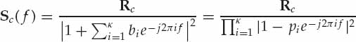
From Eqn. (11.7), it follows that the clutter cross-spectral matrix Sc(f) can be expressed as in Eqn. (11.8), where Rc defines the spatial distribution of the cold clutter, and r(τ) determines its Doppler power spectrum structure according to the scalar function sc(f). The clutter Doppler power spectrum at the conventional beamformer output, is given by p(ϕ0, f) = s†(ϕ0)Sc(f)s(ϕ0) = [s†(ϕ0)Rcs(ϕ0)]sc(f). The scale of this spectrum may change with radar look direction ϕ0 since Rc is typically not equal to the identity matrix. However, the structure of this spectrum has the same form sc(f) independent of the steer angle ϕ0. From a physical viewpoint, this implies that there is no angle-Doppler coupling in the cold-clutter spectrum to within a complex scalar. While such a model is often quite appropriate for OTH radar in an approximate sense,2 it is clearly not valid for the airborne microwave radar case. Despite the analogies drawn between these two radar systems with respect to the hot-clutter problem in Abramovich et al. (1998), it may be expected that any fast-time STAP approach based strongly on this type of clutter model will probably not be directly appropriate for airborne radar.
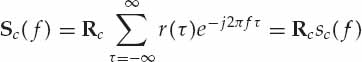
(11.8)
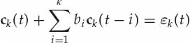
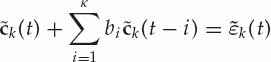
Once it has been accepted that the clutter correlation properties can be written as Eqn. (11.7), or equivalently in Eqn. (11.8), statistical realizations of the Gaussian distributed clutter process ck(t) may be generated using the scalar multi-variate auto-regressive (AR) model defined in Eqn. (11.9). The order of this model κ depends on the characteristics of the clutter slow-time auto-correlation coefficient function r(τ). Based on experimental observations of skywave OTH radar clutter, empirical analysis suggests that the snapshots ck(t) may be statistically modeled quite accurately using a relatively low-order AR model, where typically κ N, as described in (Abramovich et al. 1998).
(11.9)
In this clutter model, the complex scalar coefficients  are the temporal AR model parameters (for range cell k), while εk(t) ∈ CN is a temporally white innovative noise vector with correlation properties given by Eqn. (11.10). The terms
  and Rc will now be discussed. Due to the relatively broad transmit beam used in OTH radar to floodlight the surveillance region, clutter received at a certain group range is returned by a spatially extended area of the Earth’s surface. This area is defined by the set of all scatterers on the locus of constant path delay within the range resolution cell limits after propagation through the ionosphere. As a result, the backscattered clutter received in any given range cell will be spatially distributed over a relatively wide angular region, such that Rc effectively has full rank. For a spatially stationary clutter process, Rc is a Toeplitz matrix with diagonal elements equal to the clutter power
  received by each antenna element.
(11.10)
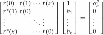
Recall that the scalar AR parameters satisfy the (κ + 1)-variate Yule-Walker equations in Eqn. (11.11), where the conjugate-symmetry property r(−τ) = r*(τ) of a wide-sense stationary process is used to define the matrix on the left-hand side. Since the zero-lag correlation coefficient r(0) = 1, by definition,  in Eqn. (11.11) is defined as the innovative noise power corresponding to an AR process output of unit variance.
(11.11)
The (κ + 1)-variate Toeplitz matrix constructed from the clutter temporal auto-correlation coefficients in Eqn. (11.11) is denoted by Rτ = Toep[r(0), r(1), …, r(κ)]. The associated AR parameter vector b = [1, b1, …, bκ]T and the innovative noise power scaling term are given by the solution of the Yule-Walker equations in Eqn. (11.12), where u1 = [1, 0, …, 0]T is the (κ + 1)-dimensional unit vector (with the first element equal to unity), and T denotes transpose.
(11.12)
The structure of the AR Doppler power spectrum is given by the parametric model sc(f) = {|B(ej2πf)|2}−1, where  is the characteristic polynomial in z = ej2πf of order κ with no roots outside the unit circle. This polynomial may also be expressed as
  , where the poles pi for i = 1, …, κ have magnitudes less than or equal to unity. Inserting this parametric description into Eqn. (11.8) yields the clutter cross-spectral matrix model of Eqn. (11.13), where f ∈ [−1/2, 1/2) is the Doppler frequency normalized by the PRF.
(11.13)
In Abramovich et al. (1998), it is assumed that the stacked clutter snapshots  may also be described by a scalar-type AR process. Provided that the AR clutter parameters in Eqn. (11.9) are locally homogeneous over a limited number of Q fast-time taps, the stacked clutter snapshots will also obey the recursive relation of Eqn. (11.14). In summary, such a model is appropriate when the clutter Doppler spectrum structure may be considered invariant over Q adjacent ranges and spatially homogeneous in cone angle to within a complex scale factor over the radar footprint.
(11.14)
It is convenient to define the N-dimensional innovative noise vector ηk(t) such that εk(t) = σεηk(t). The NQ-variate stacked innovative noise vector may then be written as  , where
  is a stacked vector of Q independent innovative noise vectors {ηk(t), ηk−1(t), …, ηk−Q+1(t)} with identical covariance matrix
  . The second-order statistics of
  can be expressed in the form of Eqn. (11.15), where the NQ × NQ block diagonal matrix
  is given by
  .
.
(11.15)
The simplest first-order (κ = 1) AR model in Eqn. (11.16) may be used to represent terrain-scattered clutter. Using Eqns. (11.11) through to (11.14), it is readily verified that the inter-pulse clutter correlation coefficient ρt = r(1) = −b1 = p1. For a stable AR process, the parameter ρt lies inside the unit circle. The modulus |ρt| < 1 determines the width of the clutter spectrum (Doppler frequency spread) due to ionospheric propagation. For κ = 1, this spectrum is parameterized by a Lorentzian profile. The argument  determines the centroid of this spectrum in frequency to reflect the mean ionospheric Doppler shift. For high PRF applications (aircraft detection missions), |ρt| → 1 in stable ionospheric conditions, with values of about 0.999 being typical for a PRF of 50-Hz. From Eqn. (11.12), we have that
  for a first-order AR process.
(11.16)
A simple model for the spatial distribution of the backscattered cold clutter assumes the covariance matrix  , where the complex scalar ρs is the inter-sensor spatial correlation coefficient of the clutter. This parameter determines the angular width of the (Lorentzian shaped) spatial spectrum and its mean DOA relative to broadside. For example, a value of ρs = 0.5 was assumed for an OTH radar footprint steered at broadside in Abramovich, Gorokhov, Mikhaylyukov, and Malyavin (1994), and Abramovich (1992). The Q independent innovative noise vectors {ηk(t), ηk−1(t), …, ηk−Q+1(t)} used to construct
  in Eqn. (11.16) may be generated by the element-space AR(1) process in Eqn. (11.17), where the superscript [n] for n = 1, …, N denotes the elements of ηk(t). Here, γn(t, k) is complex driving white Gaussian noise with correlation properties given by
  .
.
(11.17)
For the case of sea-surface scattering, a second-order (κ = 2) AR model may be proposed to represent the two dominant Bragg lines in the clutter Doppler spectrum. The values of κ = 1 and κ = 2 (corresponding to the simplest terrain and sea-clutter AR models, respectively) are therefore minimum model order requirements. In practice, higher-order models are often required to capture the received clutter Doppler spectra more accurately. A basic parameter set for modeling sea-surface clutter at low (ship-detection) PRFs of about 5-Hz has been specified as b1 = −1.9359, b2 = 0.998,  in Abramovich (1992) and Abramovich (1994).
While the value of κ may be selected a priori based on the expected characteristics of the clutter, the model parameters  will be unknown in general. Moreover, cold-clutter signals may be partially or fully submerged by the hot clutter in an operational system. In this case, access to cold clutter-only snapshots is not directly available in practice for identifying (estimating) the AR model parameters.
11.2.3 Hot Clutter
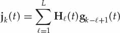
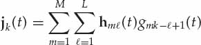
Hot clutter is assumed to arise from a convolutive mixture of M external interference sources emitting independent complex scalar waveforms denoted by gmk(t) for m = 1, …, M. The received hot-clutter spatial snapshot jk(t) may be written as the multichannel discrete convolution in Eqn. (11.18), where L is the maximum duration of the hot-clutter channel impulse response in fast-time samples for the source with the largest multipath time dispersion. In other words, the multipath components received from the M hot-clutter sources are contained within a differential group-range interval of ΔR = cL/fs. Although L may loosely be referred to as the maximum number of paths or ionospheric modes over all M sources, it is more accurate to interpret L as the maximum fast-time sample interval between loci of constant path-delay in the case of continuously distributed scatterers. The complex multi-channel FIR function that links source m to the N antenna elements is denoted by the N-variate vector hm (t) for = 1, …, L. The channel impulse response coefficients in hm(t) may be considered essentially frozen in fast-time k (i.e., over the relatively short PRI), but they may fluctuate with respect to slow-time t over the relatively long CPI. The rate of channel “non-stationarity” is related the highest differential Doppler shift between the scatterers on each loci of constant path delay (Fante and Torres 1995).

(11.18)
The hot-clutter array snapshot vector jk(t) is more conveniently expressed in the form of Eqn. (11.19). Here, the M-dimensional signal vector gk(t) = [g1k(t), …, gMk(t)]T contains the complex source waveforms received at fast-time k and slow-time t, while the N × M matrix H(t) = [h1(t), …, hM(t)] represents the instantaneous total impulse response of the hot-clutter channel at fast-time delay . This matrix remains constant during the “quasi-instantaneous” PRI but changes as the channel evolves in slow-time t over the CPI. More specifically, the (n, m)th element of H(t) contains the complex scalar channel coefficient that transfers source m to receiver n at relative delay in repetition period t. In the hypothetical case of no multipath L = 1, Eqn. (11.19) reverts back to the familiar instantaneous mixture model jk(t) = H(t)gk(t), where the columns of the mixing matrix H(t) = [h1(t), …, hM(t)] may be regarded as the M interference wavefronts received at slow-time t.
(11.19)
The source waveforms gmk(t) are assumed to be mutually independent with correlation properties in Eqn. (11.20), where rm(k) is the fast-time auto-correlation function of the mth hot-clutter source and * denotes complex conjugate. As the power of each hot-clutter signal (mode) will be accounted for in the channel impulse response definition later on, the source waveforms may be scaled to unit variance (rm(0) = 1) without loss of generality. Unless otherwise stated, we shall assume broadband sources with an essentially flat power spectral density over the jammer bandwidth Bm > fs = 1/Ts, such that rm(k) = δ(k). In the final section of this chapter, interference sources with narrow band-widths in the interval 1/Tp = fp  Bm < fs will be considered, such that |rm(k)| → 1 for kTs Tp.
(11.20)
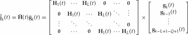
Now consider the NQ-variate stacked hot-clutter vector  , which may be expressed in the compact form of Eqn. (11.21). Here,
  is the M(L+Q−1)-variate stacked vector of {gk(t), gk−1(t), … gk−L+1−Q+1(t)}, while
  is an NQ × M(L + Q − 1) block-Sylvester matrix constructed from the matricies {H1(t), …, HL(t)}. It may be readily verified that the expression for
  in Eqn. (11.21) is consistent with the definition of the individual spatial snapshots {jk(t), jk−1(t), …, jk−Q+1(t)} in Eqn. (11.19), which form the stacked hot-clutter vector.
(11.21)
Using Eqn. (11.21), the NQ × NQ hot-clutter covariance matrix 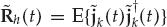 is given by Eqn. (11.22), where
  is the associated source covariance matrix. The matrix
  is slow-time varying due to the dynamic channel impulse responses over the CPI. However, it may be regarded essentially constant in fast-time over a relatively short PRI, which effectively observes a “quasi-instantaneous” snapshot of the channel fluctuations.
For independent broadband jamming signals, the source covariance matrix has full rank given by  , where the operator R{·} returns the rank of a matrix. As the dimensions of the system matrix
  are NQ × M(L + Q − 1), it follows that the (noise-free) NQ × NQ hot-clutter covariance matrix is guaranteed to be rank deficient when NQ > M(L + Q − 1), where we recall that L is defined as the maximum impulse response duration over all M sources.
(11.22)
The rank deficiency of for dimensional parameters satisfying the condition in Eqn. (11.23) has important implications for hot-clutter rejection. Specifically, it means that a fast-time STAP architecture of dimension NQ has sufficient DOFs to cancel the hot clutter effectively when the filter is updated on a pulse-by-pulse basis. In conditions of no multipath L = 1, Eqn. (11.23) holds only if the number of antenna elements is greater than the number of independent sources N > M, which confirms that fast-time STAP has no scope to outperform SAP in the absence of multipath. Indeed, the condition in Eqn. (11.23) holds only if N > M, irrespective of the values of L and Q, i.e., the maximum number of independent sources that can be effectively canceled by both SAP and fast-STAP must be less than the number of antenna elements. In the case of pure SAP (Q = 1), Eqn. (11.23) suggests that hot clutter can be effectively canceled when N > ML. As not all sources will have the maximum impulse response length L in practice, the milder condition 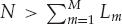 applies, where Lm is the duration of source m. There is another subtle point; while Eqn. (11.23) indicates the potential for effective hot clutter cancelation using fast-time STAP filters updated in slow-time, a generalized “main beam” scenario may unfortunately result if the stacked useful signal vector
  is accurately spanned by the hot-clutter subspace, i.e., as a linear combination of the columns of . In this case, hot-clutter rejection is still possible, but the signal-to-hot-clutter ratio will be degraded.
(11.23)
The condition in Eqn. (11.23) may be interpreted as a fast-time STAP generalization of the spatial-only condition N > M necessary for the effective rejection of independent interference sources by SAP. This expression may be recast in the form of Eqn. (11.24), which allows the designer to determine the minimum number of fast-time taps necessary to ensure that the (quasi-instantaneous) stacked hot clutter-only covariance matrix is rank deficient for a given number of sources M and maximum impulse response duration L. The number of taps Q = L, typically adopted as a rule-of-thumb, can only guarantee rank deficiency of for the case M < N/2, i.e., when the number of independent sources is less than half the number of antenna elements. For M N/2, values of Q < L are sufficient, which is a less restrictive condition than the rule-of-thumb. Whereas for the maximum number of independent sources that can possibly be canceled Mmax = N − 1, the number of fast-time taps required to ensure rank deficiency of is Qmax = Mmax(L − 1) which is typically greater than L in practical scenarios. Clearly, SAP will be ineffective for cases where Q > 1 taps are required for rank deficiency in Eqn. (11.24).
(11.24)
Having described the underlying conditions for which fast-time STAP has the potential to effectively cancel hot clutter and outperform SAP, we may now consider specific models that may be used to simulate the hot-clutter signal. Based on the work of Abramovich, Spencer, and Anderson (1998), and real-data processing results presented for the ionospheric HF channel in the second part of this text, a modified version of the generalized Watterson model (GWM) may be used to simulate the channel vectors hm(t) that give rise to the “non-stationary” hot-clutter phenomenon. In array processing terminology, hm(t) in the model of Eqn. (11.25) may be regarded as the hot-clutter “wavefront” received in PRI t from source m for the mode with relative delay . Note that the sum is over the maximum number of paths = 1, …, L for all sources, but it is clear that hm(t) = 0 for > Lm, i.e., when the fast-time delay exceeds the impulse response duration of source m.
(11.25)
The slow-time varying channel vectors hm(t) are assumed to be random and statistically independent for different sources and modes. In the GWM model of Eqn. (11.26), the terms Am and fm denote the RMS amplitude and Doppler shift of mode from source m, respectively, while the N × N matrix Sm represents the mean synthetic wavefront of this mode over the CPI (as described below). The multi-variate complex Gaussian distributed N-dimensional vector cm(t) encapsulates the random space-time fluctuations of the received hot-clutter wavefronts. This accounts for the DOA and Doppler spread imposed on the various sources and modes. In Chapter 8, the simplest model for cm(t) was described as a Markov chain defined by two parameters, namely, a temporal correlation coefficient αm, and a spatial correlation coefficient βm, both real-valued quantities in the interval between zero and one. Lower values of αm and βm correspond to diffusely scattered modes with faster temporal fluctuations and greater wavefront variability. In other words, the parameters αm and βm represent the prevailing characteristics of the different ionospheric paths responsible for producing the hot-clutter signal. Specific values of αm and βm will be quoted in Section 11.3.3 for individual hot-clutter modes.
(11.26)
The only modification to the GWM described in Chapter 8 relates to the definition of Sm. When diffuse scattering occurs from a rough ionospheric surface, the resulting hot-clutter “mode” is not reflected from a single point hence the mean wavefront will not be planar. In this case, signal components arriving with similar path delay may be due to a continuum of point scatterers that are spatially distributed over an extended region. These “micro-multipath” components received from scatterers along a locus of constant path delay superimpose to produce a synthetic wavefront, which may deviate significantly from a plane wave. The assumption of a mean plane-wavefront model is therefore not suitable for these hot-clutter modes.
In Abramovich et al. (1998), it is proposed to define Sm based on the Karhunen-Loève expansion of the hot-clutter mode spatial covariance matrix Fm averaged over an infinite time interval in Eqn. (11.27). While the spatial rank of a single hot-clutter mode is assumed to be unity in any given repetition period, it is noted that the time-averaged spatial covariance matrix of a single hot-clutter mode tends to full rank when it is integrated over a relatively long CPI because of the mode wavefront structure variations embodied in the slow-time varying channel vector hm(t).

(11.27)
The NQ × NQ space/fast-time covariance matrix 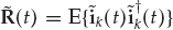 , defined in terms of the stacked hot-clutter-plus-noise vector
  , has the block-Toeplitz structure in Eqn. (11.28), where the N × N blocks are given by the fast-time lagged hot-clutter-plus-noise spatial covariance matrices
 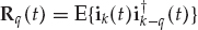 for sample lags q = 0, …, Q − 1 in the fast-time tap delay line.
(11.28)
Specifically, the matrix blocks are given by Rq(t) = E{[jk(t) + nk(t)][jk−q(t) + nk−q(t)]†}, and expanded further in Eqn. (11.29), where the assumption of independence between the composite hot-clutter signal and additive noise is invoked to separate the two expectations.

(11.29)
The mutual independence of the individual hot-clutter sources and modes means that all the cross-terms in Eqn. (11.29) cancel. Eliminating these terms, and substituting hm(t) for its definition in Eqn. (11.26), the standard spatial covariance matrix corresponding to zero fast-time lag (q = 0) is given by Eqn. (11.30). Recall that the additive noise nk(t) is assumed to be spatially white of power  , such that
  .
.
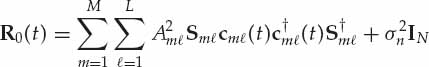
(11.30)
For q = 1, …, Q − 1, the fast-time lagged spatial covariance matrices Rq(t) are given by Eqn. (11.31). The additive noise component doesn’t appear because E{nk(t)nk−q(t)†} = 0 for q > 0. Since the hot-clutter source waveforms are assumed to be temporally white in the broadband case, the only hot-clutter contributions in Rq(t) are from pairs of modes that have a differential path delay of q fast-time samples. Clearly, Rq(t) = 0 for q ≥ L since there is no pair of modes with a differential delay exceeding the maximum impulse response duration of the hot-clutter channel.
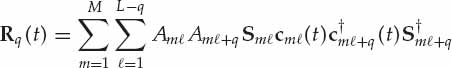
(11.31)
11.3 Mitigation Techniques
Most schemes for hot- and cold-clutter mitigation are based on a cascaded processing approach in which a hot-clutter canceler, typically a fast-time STAP technique, precedes a cold-clutter suppression stage, either implemented as a slow-time STAP technique or standard Doppler processing. In airborne radar applications, this processing sequence is largely motivated by practical considerations, including training strategies and computational complexity. In OTH radar, such processing is additionally motivated by the cold-clutter properties, which in general allow it to be mitigated effectively by standard Doppler processing. For this reason, the cascaded approach in which fast-time STAP for hot-clutter cancelation is followed by standard Doppler processing for cold-clutter suppression is considered.
Standard fast-time STAP techniques may be broadly distinguished in terms of whether the filter weights are held fixed or updated within the CPI. Intra-CPI filter adaptations are primarily motivated by the need to track the time-dependence or “non-stationarity” of the hot-clutter space/fast-time covariance matrix over the relatively long radar dwell. However, the deleterious impact of a STAP filter that changes during the CPI on the subsequent cold-clutter suppression stage is not always taken into account. The scope of this section is to describe fast-time STAP techniques applicable for hot-clutter cancelation in pulse-waveform (PW) and continuous waveform (CW) OTH radar systems. Methods required to tailor such techniques to the peculiarities of airborne radar systems will not be discussed here.
Only a handful of studies have specifically addressed the design of the cascaded approach in which the slow-time varying STAP filter for hot-clutter rejection is synthesized with due regard to the effect on the performance of the subsequent cold-clutter canceler. The first part of this section recalls standard fast-time STAP techniques based on static and dynamic filters over the CPI. Alternative fast-time STAP techniques that overcome the limitations of these standard approaches are then described in the second part of this section. The third part of this section compares the performance of standard and alternative processing schemes using simulated data.
11.3.1 Standard Schemes
Two basic types of standard fast-time STAP filters may be identified. The first adopts a fixed weight vector  to process all ranges and pulses in the CPI. This filter varies only with radar look direction ϕ0, but this dependence is considered implicit and omitted here for notational convenience. The second is based on a slow-time dependent filter
  that processes all range bins in pulse t for t = 1, …, P. The most general STAP filter, denoted by
  , is both slow-time varying and range dependent. This type of filter will be discussed in the second part of this section, which describes alternative STAP techniques.
The majority of STAP techniques described in the open literature are based on the solution of a linearly constrained minimum variance (LCMV) optimization problem, which incorporates multiple linear constraints. The LCMV formulation is a generalization of the more familiar minimum variance distortionless response (MVDR) approach, which incorporates a single linear constraint. The LCMV optimization problem may be written as Eqn. (11.32). Here, the argument w ∈ CNQ is the weight vector of the (generic) fast-time STAP filter, R normally represents the NQ × NQ hot-clutter-plus-noise covariance matrix, while the NQ × q constraint matrix C, and the q-dimensional response vector f, define the q linear constraints imposed on the filter w.
(11.32)
The optimum solution wo is the weight vector that minimizes the interference power w†Rw at the STAP output subject to the q linear constraints w†C = f†. This filter is given by Eqn. (11.33), where the matrix R is assumed to be positive definite, so that R−1 exists. The derivation of this solution using the method of Lagrange multipliers can be found in Frost (1972). We shall find it useful to refer back to this general expression and assign specific definitions to the various terms in Eqn. (11.33). The terms R, C, and f conveniently serve as “place-holders” for now. It is mainly with regard to these definitions, and the manner in which filter is implemented, that the standard and alternative fast-time STAP approaches differ.
(11.33)
11.3.1.1 Linear Deterministic Constraints
Traditionally, the main purpose of the linear constraints is to ensure that the filter provides fixed gain and distortionless processing of useful signals incident from the look direction ϕ0. Standard fast-time STAP techniques typically employ deterministic constraints for this purpose. Different approaches have been proposed to protect the useful signal from attenuation and distortion at the fast-time STAP output. To motivate these approaches, it is instructive to express the stacked useful signal vector  in the form of Eqn. (11.34). With reference to the spatial snapshot model in Eqn. (11.2), the Q-variate fast-time vector ψk = [ψk, ψk−1, …, ψk−Q+1]T contains the useful signal samples in the Q-tap delay line of the STAP filter, while the NQ × Q matrix AQ(ϕ0) is given by AQ(ϕ0) = s(ϕ0) ⊗ IQ, where ⊗ denotes Kronecker product.
(11.34)
Now consider the case of q = Q linear deterministic constraints with the constraint matrix defined as C = AQ(ϕ0). To determine the effect on the useful signal, assume that a generic fast-time STAP filter w satisfying the condition w†C = f† processes the useful signal vector . Using Eqn. (11.34), it is readily determined that the scalar output  is given by Eqn. (11.35), since the condition w†A(ϕ0) = f† is enforced by the constraints matrix C = A(ϕ0). In this case, it is observed that the STAP output sk(t) depends on the Q-variate response vector f through the inner product f†ψk. As pointed out in Griffiths (1996), the complex scalar f†ψk may be interpreted as the output of a correlation receiver applied in the fast-time sample domain, where the filter coefficients of this receiver are given by the elements of the response vector f.
(11.35)
Two cases are of particular interest. The first is the matched-filter receiver, given by f = αψk for an arbitrary constant α, which maximizes the signal-to-white-noise ratio in the output sk(t). The second is the receiver that provides fixed unity gain and distortionless coherent processing to yield the output sk(t) in Eqn. (11.36). The latter is clearly obtained by setting the first element of f to unity and the other Q − 1 elements to zero, i.e., f = eQ = [1, 0 …, 0]T, such that f†ψk = ψk. Ideally, a pulse-compressed useful signal is impulsive in fast-time when range sidelobes are ignored. When such a signal is matched to the current range k, we have that ψk = [1, 0, …, 0]T. In this case, the matched filter receiver coincides with the distortionless response receiver f = eQ.
(11.36)
Hence, the Q linear deterministic constraints defined by C = AQ(ϕ0) and f = eQ represent a minimum requirement to ensure fixed unit gain and distortionless processing of an ideal useful signal at the output of a fast-time STAP filter. If it is desired to make the output useful signal sk(t) more robust to pointing errors, a corresponding constraint on derivatives might also be imposed, e.g., by setting C = A2Q(ϕ0) defined in Eqn. (11.37), and f = e2Q, where  . We may write C = Aq(ϕ0) and f = eq for the general case of q > Q linear deterministic constraints.

(11.37)
The use of a single linear deterministic constraint has been advocated in certain fast-time STAP studies. To motivate this concept, it is more convenient to express the stacked useful signal vector in the alternative form of Eqn. (11.38), where the NQ-variate vector ψk ⊗ s(ϕ0) is substituted for the equivalent matrix multiplication AQ(ϕ0)ψk in Eqn. (11.34). For an ideal target echo matched to the current range cell k, we impose the condition ψk = eQ in Eqn. (11.38) such that , where the vector v(ϕ0) = eQ ⊗ s(ϕ0) is regarded as the space/fast-time steering vector.
(11.38)
It would appear that the single linear constraint defined in Eqn. (11.39) suffices in this case. Indeed, this constraint provides unit gain to a useful signal when the location of the impulse is matched to the current range k. However, as the fast-time STAP filter “slides over” different fast-time samples to process different range cells k, the location of this impulse moves into a subsquent tap of the delay line that trails the current range cell processed. In these trailing taps, the spatial response of the antenna weights in the direction ϕ0 is unconstrained when only the constraint in Eqn. (11.39) is imposed. The spatial response of the processor to the useful signal in these taps will in general be nonzero and may fluctuate over pulses if the weight vector is updated within the CPI. This causes a degradation in the range-sidelobe structure of useful signals at the fast-time STAP output. Visually, the processed target echo may appear spread or “smeared” in range over the full length Q of the fast-time tap delay line. In the case of a dynamic filter that is updated from pulse to pulse, temporal variations in the range sidelobe structure over the PRI will additionally cause these sidelobes to appear spread in Doppler.
(11.39)
In summary, a single linear constraint can provide unit gain to matched useful signals but cannot ensure distortionless processing of such signals. For this reason, the set of Q linear deterministic constraints defined previously is recommended for fast-time STAP. The first of these linear constraints provides fixed unity gain to useful signals incident from the radar look direction. This not only protects a useful signal matched to the current range from being inadvertently attenuated, but also ensures Doppler coherence of the target echo across the different repetition periods in the CPI. On the other hand, the remaining Q − 1 constraints ensure the fast-time STAP filter has zero response in the look direction over the trailing taps of the delay line to avoid smearing the output useful signal energy in range (and in Doppler for a time-varying filter).
11.3.1.2 Time-Invariant STAP
The first standard fast-time STAP approach to be described is based on a time-invariant weight vector held fixed over the CPI. The optimum (time-invariant) STAP filter is given by in Eqn. (11.40), where  is the hot-clutter-plus-noise covariance matrix averaged over the CPI. To arrive at the solution , the term R in Eqn. (11.33) is substituted for
  , while the linear deterministic constraints are defined by C = Aq(ϕ0) and f = eq. The filter is optimum in terms of output signal-to-hot-clutter-plus-noise ratio when conditioned on the set of all time-invariant filters.
(11.40)
Stacked hot-clutter-plus-noise training snapshots are required to estimate the unknown matrix . In an OTH skywave radar system, a limited number of practically clutter-free snapshots may be found near the start of the PRI (i.e., at short ranges) due to the skip-zone phenomenon. Whereas in an HFSW radar system, the high attenuation of the surface-wave at long ranges often permits clutter-free snapshots to be obtained near the end of the PRI. In any case, this allows for supervised training using Nk hot-clutter-plus-noise-only snapshots  available in each PRI, where Nk < K. Using the first Nk range cells, e.g., the unknown matrix may be estimated as
  in Eqn. (11.41).

(11.41)
Diagonal loading is often not necessary when the sample covariance matrix is averaged over the whole CPI, as typically PNk 2NQ. The main issue relates to the rank-expansion of over the relatively long CPI and the inability of the associated STAP filter to effectively cancel non-stationary hot clutter. Specifically, the adaptive implementation of this first standard approach is denoted by the time-invariant STAP filter ŵ in Eqn. (11.42), which is used to process all ranges and pulses in the CPI. This approach shall be referred to as time-invariant STAP hereafter. As discussed previously, the number of deterministic constraints may be q = Q or q = 2Q, depending on whether robustness to beam-pointing errors is deemed neccessary.
(11.42)
Similar concepts to those described above for PW systems also apply to CW systems after range processing is performed. It is shown in Abramovich et al. (2000) that range processing by FMCW deramping and FFT-based spectral analysis does not effect the hot-clutter-plus-noise covariance matrix model in Eqn. (11.22) under relatively mild assumptions that normally hold in practice. Hence, fast-time STAP techniques described in this and the following sections are applicable to both PW and CW OTH radars when supervised training is possible.
Depending on system characteristics and propagation conditions, it may occur that all range bins contain significant cold-clutter contributions. In this unsupervised training scenario, it is desirable to perform pre-processing to attenuate the cold-clutter signal prior to hot-clutter covariance matrix estimation. A scheme that makes use of an MTI clutter removal filter to obtain suitable training data is described in Abramovich et al. (2000).
11.3.1.3 Unconstrained STAP
Now let’s turn our attention to the specification of the optimum slow-time varying STAP filter denoted by . In this case, the term R in Eqn. (11.33) is substituted for the quasi-instantaneous hot-clutter-plus-noise covariance matrix  defined in Eqn. (11.28), while the linear deterministic constraints are defined by C = Aq(ϕ0) and f = eq, as before. The slow-time dependent optimum filter is given by Eqn. (11.43).
(11.43)
Since the hot clutter is assumed to be stationary over the quasi-instantaneous PRI, the STAP filter is optimum in terms of output signal-to-hot-clutter-plus-noise ratio. In practical applications, the hot-clutter-plus-noise covariance matrix is unknown, but may be estimated as  in Eqn. (11.44). Here, only the training range cells in the current PRI are used. Diagonal loading at an appropriate level σ2 is often applied to improve convergence rate in conditions of low sample support when Nk < 2NQ.
(11.44)
The true covariance matrix may be substituted for the regularized sample estimate in the optimum filter expression of Eqn. (11.43) to yield the adaptive STAP filter ŵ(t) in Eqn. (11.45). This practical filter is used to process the operational range cells k = Nk + 1, …, K in the current PRI t. This approach is characterized by relatively higher computational complexity compared to time-invariant STAP, but is potentially more effective for non-stationary hot-clutter cancelation provided that the condition NQ > M(L + Q − 1) is met. This second standard approach is referred to as unconstrained STAP in the sense that the weights may vary arbitrarily in slow-time t aside from the q linear deterministic constraints.
(11.45)
Although the deterministic linear constraints protect the gain and Doppler spectrum of signals incident from the radar look direction, the (otherwise unconstrained) changes in  over the CPI will temporally modulate cold-clutter returns incident from other directions. This is because the response of is unconstrained in all directions but the look direction, and is therefore free to fluctuate in an uncontrolled manner from pulse to pulse.
11.3.1.4 Relative Merits and Shortcomings
In summary, two standard operational fast-time STAP techniques have been motivated and described. The first is referred to as the standard time-invariant STAP scheme, which corresponds to the static adaptive filter ŵ in Eqn. (11.42). This approach has the advantage of relatively low computational complexity and reduced demands on sample support for practical implementation. Importantly, use of a fixed filter to process the CPI also preserves the temporal inter-pulse correlation properties of the cold clutter at the fast-time STAP output. This is vital for effective cold-clutter mitigation in the subsequent Doppler processing step.
The main problem with this approach is that it often cannot effectively reject non-stationary hot clutter because the sample covariance matrix has large or full rank when averaged over a typical OTH radar CPI. In practice, this scheme may be regarded appropriate when the non-stationarity of the hot clutter is not significant on the scale of the CPI. Real-data processing results suggest that this typically corresponds to CPI lengths which are too short for OTH radar purposes, particularly for (but not limited to) ship-detection applications.
The other standard method, referred to as unconstrained STAP, is based on the slow-time varying adaptive filter ŵ(t) in Eqn. (11.45). While this scheme is typically able to reject the hot clutter effectively, the slow-time modulation induced on the cold-clutter output by the STAP filter updates will in general preclude effective cold-clutter suppression via Doppler processing. Indeed, application of the standard unconstrained STAP filter often has a devastating effect on SCV after Doppler processing. Diagonal loading heavier than required to improve the convergence rate may be applied to stabilize the fluctuations of ŵ(t). This method can improve the inter-PRI correlation properties of the cold clutter at the STAP output. However, for sufficiently non-stationary hot clutter, no level of diagonal loading can simultaneously provide effective hot-clutter mitigation and distortionless processing of the cold-clutter signal.
If the cold clutter were generated by a small number of point scatterers, its Doppler spectrum properties could be preserved by imposing a limited number of additional linear deterministic constraints that freeze the STAP filter response in the direction of each point scatterer (Griffiths 1996). As explained in Abramovich et al. (2000), the spatial distribution of the cold clutter is generally quite broad, so the backscattered radar signal enters through a large part of the receiving antenna pattern rather than from a few discrete directions only. Hence, the addition of deterministic linear constraints is not a feasible solution since it is not possible to hold constant all or most of the antenna pattern without incurring a dramatic degradation in non-stationary hot-clutter rejection.
11.3.2 Alternative Procedures
Only a few studies have specifically addressed the problem of preserving the natural slow-time correlation properties of the spatially broadband cold clutter at the STAP filter output while simultaneously updating the weight vector in slow-time to counter the non-stationarity of hot clutter. Perhaps the first attempt to provide a solution to this problem was reported in Anderson et al. (1997) and Abramovich, Spencer, and Anderson (1998) for supervised training scenarios, and subsequently in Abramovich et al. (2000) for unsupervised training. The pioneering work of Abramovich in this area represents a generalization of specific methodologies described in Abramovich et al. (1994) for spatial-only adaptive processing. The main objective of this approach, known as the stochastically constrained fast-time STAP or SC-STAP method, is to effectively cancel non-stationary hot clutter while preserving the slow-time correlation properties of the clutter output for coherent Doppler processing. The SC-STAP method is briefly recalled in this section. Further details can be found in Klemm (2004).
Motivated by practical considerations and the high computational load associated with the SC-STAP method, this section introduces a new approach called time-varying STAP or TV-STAP, which provides an attractive alternative for real-time implementation. With respect to the SC-STAP method, the TV-STAP approach allows the computational load to be significantly reduced in situations where the hot clutter can be effectively canceled by STAP filters updated at a rate slower than every PRI. Importantly, the reduced computational load is not traded-off against hot-clutter cancelation performance in this case.
Both SC-STAP and TV-STAP have been designed with OTH radar applications in mind, as they both rely in an approximate sense on the aforementioned cold-clutter model. Consequently, the SC-STAP and TV-STAP techniques described below are not directly applicable to airborne radar systems, where cold clutter exhibits strong angle-Doppler coupling due to platform motion and is more accurately represented by a multi-variate (as opposed to a scalar-type) AR model. A slow-time dependent STAP filter that can address the airborne radar problem has been proven to exist in theory; see Abramovich et al. (1998). However, operational versions of this approach will not be discussed here.
11.3.2.1 Stochastically-Constrained STAP (SC-STAP)
The full details of the stochastic constraints (SC) technique for fast-time STAP are not repeated here for brevity, but an overview of the approach is given for two main reasons: (1) to provide motivation for the development of the subsequent TV STAP algorithm, and (2) to explain the similarities and differences between TV-STAP and the SC-STAP method.
The key idea behind SC-STAP is to apply a PRI-varying and range-dependent filter that is able to preserve SCV by statistically approximating the condition 
 at the cold-clutter output, where
  is a fixed reference STAP weight vector that provides distortionless cold-clutter processing. Clearly, the SC-STAP filter
  differs from and changes over the CPI to effectively reject non-stationary hot clutter. Utilizing the κth order scalar-type AR model for the stacked cold-clutter snapshots
  in Eqn. (11.14), the scalar cold-clutter output ck(t) of the SC-STAP filter is given by Eqn. (11.46).

(11.46)
Inspection of Eqn. (11.46) reveals that the terms in the summation may be made identical to those processed by a stable filter provided that the weight vector satisfies κ linear stochastic constraints in Eqn. (11.47). If this weight vector also satisfies the quadratic constraint  , where
  , the power of the output innovative noise in Eqn. (11.46) is also equalized. The scalar innovations
  and
and  will correspond to different white-noise realizations, i.e.,
  , but the stochastic constraints ensure that the cold-clutter processes
  and
and  are statistically equivalent under these conditions. In this case, the scalar cold-clutter output ck(t) processed by the filter is statistically identical to the cold-clutter output of the stable filter . Consequently, ck (t) is described by a stationary κth order AR model with the same parameters
  as those of the input slow-time sequence of cold-clutter stacked vectors defined in Eqn. (11.14). The important point is that the requirement to preserve the auto-regressive correlation properties of the cold clutter at the STAP filter output does not necessarily imply that the STAP filter needs to be time invariant.
(11.47)
These fundamental observations made in Abramovich et al. (1998), as well as in earlier references therein for the case of pure spatial filtering, provide scope for the weight vector to change over the CPI in response to hot-clutter non-stationarity, while simultaneously stabilizing the auto-regressive cold-clutter characteristics at the output of the fast-time STAP filter. It follows that the optimum SC-STAP filter may be synthesized according to Eqn. (11.48) using the matrix  defined in Eqn. (11.49).
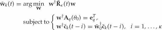
(11.48)
The linear deterministic constraints  are applied for the same reasons as in the two standard STAP schemes. In Eqn. (11.49), is defined as the hot-clutter-plus-noise covariance matrix averaged over κ + 1 adjacent repetition periods. This sliding-window average terminates at pulse t and moves forward one pulse at a time until the end of the CPI is reached, i.e., t = κ + 1, …, P. The first matrix in the sequence is denoted by
  . Since κ N, the average is performed over a relatively small number of adjacent pulses in which the true hot-clutter-plus-noise covariance matrix may be regarded as locally stationary, i.e.,
  .
.
(11.49)
The initial filter of the SC-STAP sequence is formed without stochastic constraints, as in Eqn. (11.50), using the matrix  averaged over the first κ + 1 PRI. This filter is independent of k and is used to process all operational range cells in the first κ + 1 PRIs, i.e.,
  for t = 1, …, κ + 1 and k = Nk + 1, …, K. Local averaging over κ adjacent PRIs does not preclude the initial filter from effectively canceling the hot clutter in the first κ + 1 pulses provided that NQ > (κ + 1)M(L + Q − 1). This is because the hot-clutter subspace dimension strictly grows by M(L + Q − 1) with every pulse averaged. Less restrictive conditions apply on the effective rank of the hot-clutter covariance matrix when the mode wavefronts vary in a highly correlated manner over adjacent PRI. The condition N > (κ + 1)P is also necessary because the apparent number of independent sources is multiplied by averaging over κ + 1 PRIs (Abramovich et al. 1998).
(11.50)
The remaining SC-STAP filters in the slow-time sequence t = κ + 2, …, P are range dependent and stochastically constrained. These SC-STAP filters are given by Eqn. (11.51), where the constraint matrix is augmented to incorporate the κ stochastic constraints  , while the response vector is extended to the form
  . The quadratic constraint mentioned earlier is not implemented in the SC-STAP approach. It has been shown that its impact is negligible in most cases, since the cold-clutter covariance matrix is generally well conditioned and the effect of weight vector fluctuations on AR innovative noise power is small (Abramovich 1992).
(11.51)
The question then becomes how to synthesize such a filter in an operational system, particularly as the cold-clutter only snapshots are not directly available to form the stochastic constraints when hot clutter is present. An operational algorithm that can closely approximate the ideal solution is derived according to the SC-STAP criterion in Eqn. (11.52). The slow-time sequence of SC-STAP filters for range cell k are formed in turn for pulses in the CPI with the current filter ŵk(t) being dependent on the filter from the previous pulse ŵk(t − 1) through the κ stochastic constraints in Eqn. (11.52).

(11.52)
In Eqn. (11.53), is defined as a regularized sliding-window estimate of the hot-clutter-plus-noise covariance matrix averaged over a length of κ + 1 repetition periods using the first Nk ranges cells as training data. This sliding-window average terminates at pulse t and moves forward one pulse at a time until the end of the CPI is reached, as before. The first matrix of the sequence is denoted by  . Similarly, the initial filter of the SC-STAP sequence is formed without stochastic constraints as
 . This adaptive filter is independent of range bin k and is used to process the first κ + 1 PRIs of the CPI, i.e., ŵk(t) = ŵ0 for t = 1, …, κ + 1 and k = Nk + 1, …, K.

(11.53)
The remaining SC-STAP filters ŵk(t) in the slow-time sequence t = κ + 2, …, P are range-dependent and stochastically constrained. These SC-STAP filters are given by Eqn. (11.54), where the constraint matrix is augmented to incorporate the κ stochastic constraints  , while the response vector is extended accordingly
  . With respect to the optimum SC-STAP filter in Eqn. (11.51), the adaptive implementation in Eqn. (11.54) involves a regularized sample estimate of the locally integrated hot-clutter-plus-noise covariance matrix , as well as the estimates of the ideal stochastic constraints given by Âq+k(ϕ0) and êq+k.
(11.54)
The operational stochastic constraints in Eqn. (11.52) are not the same as the ideal ones in Eqn. (11.47), but they can approximate them well when the hot-clutter component is effectively rejected by the weight vectors ŵk(t) over a window length of κ PRI. Provided that the residual hot clutter plus noise is small compared to the processed cold clutter contribution, the adaptive SC-STAP filter output may be approximated as Eqn. (11.55). By setting  for i = 1, …, κ and t = κ + 2, the second weight vector in the SC-STAP sequence provides a good approximation to the ideal condition in Eqn. (11.47). The same follows for the remaining SC-STAP filters in the slow-time sequence t = κ + 3, …, P. This is because all weight vectors in the chain are ultimately referenced to ŵ0 by virtue of the iterations. As far as useful signals are concerned, the deterministic linear constraints ensure that
 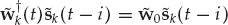 for all SC-STAP weight vectors.
(11.55)
The main point is that clutter-only snapshots are not necessary to approximate the stochastic constraints in this operational routine. Moreover, the unknown AR clutter parameters are only required to be locally stationary over κ + 1 successive pulses for the stochastic constraints to preserve the output cold clutter correlation properties.
11.3.2.2 Time-Varying STAP (TV-STAP)
In an attempt to stabilize the AR spectral characteristics of the cold clutter output, the SC method forms a new adaptive filter every PRI in a “sliding window” fashion using a different set of linear stochastic constraints, such that for an AR process of order κ, the SC-STAP weights are updated a total of P − κ times over the CPI. This effectively means that the filter coefficients are updated at a rate equal to the PRF, irrespective of the physical duration of the waveform repetition period or the prevailing hot-clutter characteristics. This rate of adaptation is mainly determined by the need to protect the AR properties of the cold clutter regardless of whether or not such fast adaptation is actually necessary for effective hot-clutter cancelation, which ought to be the primary reason for updating the weight vectors.
In high PRF (aircraft detection) applications, or when the ionospheric propagation channels are not changing rapidly, the hot clutter may have a local stationarity interval which significantly exceeds a single PRI. This can be exploited to update the weights less frequently over the CPI with practically no loss in hot-clutter rejection performance. In this situation, the SC-STAP technique has at least one major drawback. That is, the procedure is computationally expensive as it requires the calculation of a separate weight solution for every PRI and range cell processed in the CPI. It is not surprising that such a scheme typically prevents real-time implementation in operational systems, particularly when the full chain of signal processing steps includes other intensive algorithms that must also be performed over a time interval less than the CPI. This issue strongly motivates the search for computationally efficient fast-time STAP techniques that can effectively address the non-stationary hot-clutter cancelation problem.
A second possible limitation, illustrated by practical examples for the case of pure spatial adaptive processing in the previous chapter, is that weight-estimation errors relative to the ideal solution occur at each filter update and accumulate over the CPI. Since these estimation errors ultimately cause a reduction in SCV after Doppler processing, minimizing the number of filter adaptations is generally preferable from the viewpoint of computational load as well as robustness to clutter Doppler spectrum broadening.
The TV-STAP method introduced in this section follows the same basic idea as the SC technique, but is structured differently to mitigate the aforementioned limitations of the original SC work. The philosophy behind TV-STAP is to update the weight vector in non-overlapping batches at a rate commensurate with the prevailing level of hot-clutter non-stationarity. Data-driven constraints are incorporated to protect the spectral integrity of the cold clutter output in accordance with an alternative clutter model to be formulated below. The main motivation of TV-STAP is to achieve comparable performance to SC-STAP, while at the same time breaking the bottleneck of real-time processing when conditions permit.
TV-STAP partitions the CPI into Nb, smaller sub-CPI or batches each containing Np pulses, and then updates the fast-time STAP weights from batch to batch rather than from PRI to PRI. For simplicity, assume that the number of batches Nb = P/Np is an integer. Selection of the batch length Np represents a compromise between smaller values (rapid updates) to counter hot-clutter non-stationarity and larger values (slower updates) to reduce computational load.
More specifically, the TV-STAP weights are adjusted using batch-integrated hot clutter plus noise covariance matrices  , which are defined in Eqn. (11.56) for b = 1, …, Nb. A salient feature of Eqn. (11.56) is that the first κ pulses in the batch that follows the current one are also included in the summation. For reasons to become apparent later, this ensures the TV-STAP filter is effective for hot-clutter rejection in the first κ pulses of the next batch. Such a modification is clearly not applied to the final batch b = Nb, as no such pulses are available (i.e., the end of the CPI is reached).

(11.56)
The TV-STAP algorithm is based on a dynamic subspace cold clutter model in the form of Eqn. (11.57). In this representation, the Np stacked cold clutter snapshots received in batch b at range k are assumed to be spanned by a stacked vector subspace of rank κ, denoted by the NQ × κ matrix  in Eqn. (11.57). Here, κ is the number of dominant spectral components resolved in the cold clutter Doppler spectrum. The Np received cold clutter snapshots are assumed to lie in the range-space of to a good approximation, where typically P > Np > κ. The κ-variate parameter vector
  contains the linear combination coefficients that define the instantaneous structure of the synthetic clutter wavefront at range k and pulse t.
(11.57)
The physical motivation behind the dynamic subspace model is that the instantaneous frequencies of the dominant cold clutter Doppler spectrum components often vary in a highly correlated manner across adjacent pulses such that the changes in phase-path for each component in slow-time may be regarded close to linear during a sufficiently short sub-CPI (batch). When the ionospheric paths propagating the cold clutter are frequency-stable, such a model may be expected to provide a fairly accurate approximation of the received clutter snapshots over a considerable number of pulses Np, i.e., Np κ. Alternatively, when the phase-path fluctuations are caused by rapid and irregular ionospheric variations that induce significant Doppler spread on the κ dominant cold clutter spectral components, the approximation will be accurate only for a relatively small number of pulses (that may not greatly exceed κ).
It is of interest to discuss the connection between the dynamic subspace representation in Eqn. (11.57) and the stationary scalar-type AR cold clutter model adopted for skywave OTH radar in Eqn. (11.58). The two may be regarded as equivalent in the absence of innovative noise  , since any snapshot resulting from the recursive sequence without such innovations can be expressed exactly as a linear combination of any other κ (linearly independent) snapshots in the same sequence.
The presence of full-rank innovative noise in the AR model implies that Eqn. (11.57) can at best only approximate the cold clutter snapshots generated by Eqn. (11.58) when Np > κ. As the innovative noise distinguishes the AR model and the dynamic subspace description, the accuracy of the approximation for Np > κ will tend to improve as the innovative noise power decreases and/or the batch length Np becomes smaller. The question arises as to whether the use of Eqn. (11.57), when the clutter actually obeys the AR model in Eqn. (11.58), results in weight-estimation errors that are comparable to those arising from the operational stochastic constraints. This issue is investigated in the simulation analysis of Section 11.3.3.

(11.58)
For the moment, let’s assume the cold clutter model in Eqn. (11.57) is appropriate. If were known, it would be possible to fix the response of the TV-STAP filter  to the clutter synthetic wavefronts received in batch b by introducing a set of auxiliary linear constraints
  for b = 2, …, Nb. Here,
  is the first weight vector in the TV-STAP sequence given by Eqn. (11.59). This weight vector is used to process the operational range cells in the first batch (b = 1) of Np pulses.
(11.59)
Such a system of constraints ensures that the dominant clutter components experience a stable filter over the entire CPI as far as the output cold clutter contribution is concerned, while leaving NQ − (q + κ) spare adaptive DOFs for effective non-stationary hot-clutter rejection at each weight update. The optimum TV-STAP weight vector for batch b is derived according to Eqn. (11.60)

(11.60)
This leads to the weight solution in Eqn. (11.61) for batches b = 2, …, Nb, where the constraint matrix and response vector are defined as  and fk(b) =
  respectively. Similar to the SC-STAP method, this set of data-driven constraints implies that all TV-STAP filters except the first one are range dependent.
(11.61)
As stated previously, the quasi-instantaneous cold clutter subspace is not directly accessible in practice due to the presence of hot clutter, so the ideal auxiliary constraints cannot be implemented. Secondly, the batch-integrated covariance matrix is unknown and must be estimated using the training range cells in each PRI. The operational TV-STAP procedure replaces the unknown matrix by its regularized sample estimate  in Eqn. (11.62).

(11.62)
As far as the constraints are concerned, development of the operational routine is based on two key observations. First, the linear independence of the cold clutter snapshots received in the first κ pulses of batch b implies that the range-space of the NQ × κ matrix is spanned by the set of vectors  . The second is that for the stacked vectors in the data matrix
  , the approximation
  is accurate provided that the TV-STAP filter effectively rejects the hot clutter in batch b, i.e.,
 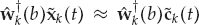 . Hence, the operational TV-STAP algorithm may be formulated in terms of q deterministic linear constraints, and κ data-driven auxiliary linear constraints, as in Eqn. (11.63).

(11.63)
This leads to the operational TV-STAP solution in Eqn. (11.64) for batches b = 2, …, Nb, where the constraint matrix  and response vector
  .
.
Analogously to SAP in the previous chapter, TV-STAP reduces the number of complex multiplications relative to SC-STAP by a factor that is closely approximated by the batch length Np. For example, if the hot clutter can be considered locally stationary over a typical surface-mode PRI with repetition frequency fp = 4 Hz, the same signal may be considered stationary over 15 consecutive air-mode PRIs when fp = 60 Hz, as the physical time interval is unchanged. In this hypothetical example, TV-STAP using Np = 16 may be expected to cancel the hot clutter as effectively as SC-STAP with an order of magnitude reduction in computational load.
(11.64)
It may be verified that for the parameter choice Np = 1, the TV-STAP algorithm reverts back to the SC-STAP method, albeit applied to the data in reverse slow-time order. In this case, TV-STAP is able to protect the cold clutter AR spectral characteristics in similar fashion to the SC-STAP method. Hence, TV-STAP may be regarded as a generalization of SC-STAP, which provides additional flexibility to reduce the computational burden when the prevailing interference environment permits (i.e., when the effective stationarity interval of the received hot clutter exceeds a single PRI). Clearly, the standard time-invariant STAP corresponds to Np = P, while the standard time-dependent STAP scheme results for Np = 1 and κ = 0. Through appropriate choices of parameters Np and κ, the TV-STAP algorithm encapsulates all STAP schemes described above as special cases, namely; the two standard STAP schemes and SC-STAP. A summary of the fast-time STAP techniques described in this section is provided in Table 11.1.
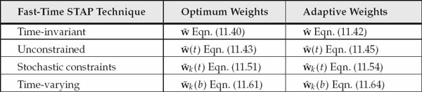
TABLE 11.1 Summary of the considered fast-time STAP techniques. Time-invariant and unconstrained STAP are standard schemes, while SC-STAP and TV-STAP are regarded as the alternative techniques. TV-STAP is most general in the sense that other techniques can be represented as special cases of TV-STAP for appropriate parameter choices.
11.3.3 Simulation Results
The simulations reported in Abramovich et al. (1998) are performed here to reproduce the numerical results described therein. In addition to ensuring consistency with the benchmark results of Abramovich et al. (1998), use of the same hot- and cold-clutter model parameters provides a fair basis on which to compare the newly proposed TV-STAP algorithm with the SC-STAP method in cases where the two techniques are not equivalent.
Once the hot and cold clutter models are defined, and the dimensions of the OTH radar data-cube are specified, the numerical analysis proceeds in three stages. The first stage examines the maximum potential effectiveness of each processing scheme in terms of hot-clutter rejection. These schemes include conventional processing, spatial-only adaptive processing (SAP), and the four previously described fast-time STAP techniques. This analysis of rejection performance is based on clairvoyant knowledge of the true hot-clutter plus noise covariance matrix. The main objective is to quantify the upper limit on hot-clutter rejection achieved by the various schemes.
The second stage investigates the impact on cold clutter processing for the schemes capable of effective hot-clutter rejection, particularly with respect to preserving SCV after Doppler processing. The synthesis of first and second stage results enables schemes that have the potential to be appropriate for hot- and cold-clutter mitigation in OTH radar to be identified. The final stage compares the performance of fully operational routines for these identified schemes. In this case, training data is used to estimate the hot-clutter covariance matrices, while cold-clutter samples are not directly available to form data-dependent constraints.
A uniform linear array (ULA) composed of N = 16 identical antenna sensors with half-wavelength inter-element spacing is considered for the simulations. The beam is steered in the broadside direction, i.e., ϕ0 = 0. As in Abramovich et al. (1998), a single far-field hot clutter source is assumed with four propagation modes, i.e., M = 1 and L = 4. The spatial and temporal parameters describing the four hot clutter modes are listed in Table 11.2. The DOA of the first hot clutter mode is intentionally chosen to lie in the main beam so as to demonstrate the benefit of fast-time STAP relative to SAP in such a scenario. Temporal parameters have been specified for low and high PRF modes in Table 11.2, where fp = 5 Hz and fp = 50 Hz are typical for OTH radar ship and aircraft detection missions, respectively.

TABLE 11.2 Hot-clutter parameters for a single (M = 1) source and four (L = 4) propagation modes.
The radar is assumed to transmit P = 256 pulses over the CPI. The model parameters corresponding to the cold clutter are listed in Table 11.3 for terrain (κ = 1) and sea surface (κ = 2) scattering. Recall that the rank of the hot clutter space/fast-time covariance matrix averaged over κ + 1 repetition periods is given by (κ + 1)M(L + Q − 1). A number of fast-time taps Q ≥ 2 is needed to cope with main beam hot clutter condition. Selecting Q = 3 results in NQ = 48 18 = (κ + 1)M(L + Q − 1) for the case of sea-surface scattering. This number of fast-time taps is sufficient to ensure that fast-time STAP has the potential to effectively reject the hot clutter.
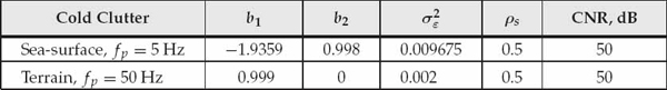
TABLE 11.3 Cold-clutter AR model parameters for terrain (κ = 1) and sea-surface (κ = 2) scattering.
11.3.3.1 Hot-Clutter Rejection
A standard metric for comparing the performance of different processing techniques is the output signal-to-hot clutter plus noise ratio (SHCR). For an ideal useful signal with unit power, the conventional matched filter beamformer s(ϕ0) yields an output SHCR given by Eqn. (11.65), where R0(t) is the statistically expected hot clutter plus noise spatial covariance matrix for pulse t. Note that the steering vector is normalized such that s(ϕ0)†s(ϕ0) = N = 16.
(11.65)
In the clairvoyant case, R0(t) is known and the optimum time-varying SAP filter takes the form of  . This shall be referred to as the standard unconstrained SAP filter. For an ideal useful signal with unit power per element, the optimum SAP filter yields a maximum instantaneous output SHCR given by Eqn. (11.66). The highest potential effectiveness is bounded above by the signal-to-white noise ratio (SWNR) at the matched-filter output when only white additive noise is present. For additive white noise of unit power per element, we have R0(t) = IN in the absence of hot clutter, so the upper bound for qSAP(t) and qCBF(t) is 10log10 N = 12 dB.
(11.66)
The output SHCR for the optimum fast-time STAP filter associated with the time-varying weight vector  that employs only linear deterministic constraints is given by Eqn. (11.67). Recall that this filter provides fixed unit gain and distortionless response for ideal useful signals in the look direction ϕ0, and that is the true hot clutter plus noise covariance matrix at pulse t. This standard technique was previously referred to as unconstrained STAP.
(11.67)
On the other hand, the output SHCR for the optimum fast-time STAP technique based on the time-invariant weight vector  , derived from the hot clutter plus noise covariance matrix
  averaged over the whole CPI, is given by Eqn. (11.68). This standard technique was previously referred to as time-invariant STAP.
(11.68)
The simulation results in Figure 11.4 illustrate the quasi-instantaneous output SHCR for the conventional beamformer, the optimum unconstrained SAP filter qSAP(t), the optimum unconstrained STAP filter qST AP(t), and the optimum time-invariant STAP filter qAVE(t), as a function of pulse number t over the CPI. Recall that the term unconstrained refers to the use of standard deterministic constraints only, i.e., without the auxiliary data-driven linear constraints used by SC-STAP and TV-STAP.

FIGURE 11.4 Optimum output SHCR of standard fast-time STAP and pure SAP approaches as a function of slow-time over the CPI. © Commonwealth of Australia 2011.
The curves in Figure 11.4 indicate the maximum potential effectiveness of the various standard techniques when estimation errors due to finite sample support are neglected. As expected, unconstrained STAP performs best. It provides an output SHCR improvement of about 60 dB with respect to the conventional beamformer qCBF(t). Moreover, it yields an output SHCR that is within about 6 dB of the upper bound on performance in this example (i.e., 12 dB).
On the other hand, unconstrained SAP is rather ineffective due to the presence of a main-beam hot-clutter component. This illustrates the susceptibility of a slow-time varying SAP filter to hot clutter, even when the number of antennas exceeds the number of independent interference components (i.e., N = 16 > 4 = ML). In this example, unconstrained SAP leads to a loss in output SHCR of around 15 dB with respect to unconstrained STAP.
Greater relative losses of approximately 30 dB are observed for time-invariant STAP, which cannot cancel non-stationary hot clutter effectively over the CPI. Among the considered standard approaches, only the fast-time STAP approach with slow-time-varying weight vectors can provide the possibility to effectively cancel non-stationary hot clutter. The other standard schemes are clearly inappropriate, even when the hot clutter statistics are perfectly known. These numerical results agree closely with those reported for an independent realization of this simulation in Abramovich et al. (1998).
11.3.3.2 Cold-Clutter Processing
From a hot-clutter rejection perspective, the standard unconstrained STAP filter performs very well. The main problem arises when this slow-time sequence of weight vectors is used to process range cells that additionally contain cold clutter. To observe the impact on processing the cold clutter only, the hot clutter is momentarily removed from the operational range cells. Figure 11.5 illustrates the cold-clutter Doppler spectrum at the output of the standard unconstrained STAP filter compared to that processed by the standard time-invariant STAP filter using the second-order AR (sea-scattering) model. The dramatic degradation in SCV is obvious when unconstrained STAP is applied. Although can effectively remove the non-stationary hot clutter, it is apparent that this filter is completely inappropriate for processing the cold clutter. The unconstrained fluctuations of destroy the pulse-to-pulse correlation properties of the scalar cold-clutter output.

FIGURE 11.5 Doppler spectra showing the sub-clutter visibility at the output of two standard STAP techniques and SC-STAP when these filters are applied to process the cold clutter. © Commonwealth of Australia 2011.
Typical target echoes have peaks that may be 40 dB below the main clutter peak in the OTH radar Doppler spectrum. Such targets are undetectable when the SCV falls to about 30 dB, as it does for the unconstrained STAP approach in Figure 11.5. In contrast, time-invariant STAP is suitable as far as cold clutter processing is concerned. This is because a static filter over the CPI avoids any degradation in SCV. However, this method relies on averaging the hot-clutter covariance matrix over the whole CPI, which leads to a degradation in rejection performance of approximately 30 dB in Figure 11.4. In this case, target echoes may not be obscured by clutter after Doppler processing, but are likely to be buried under the high residual hot-clutter level.
The simulation results presented thus far demonstrate that both standard fast-time STAP approaches (i.e., unconstrained and time-invariant) are ineffective for the considered problem, as neither can simultaneously yield effective hot-clutter rejection and distortionless cold-clutter processing.
The cold-clutter Doppler spectrum processed by the optimum SC-STAP technique using two stochastic constraints for the AR(2) sea scattering model is also illustrated in Figure 11.5. Ideal stochastic constraints were constructed using pure cold clutter snapshots and are therefore non-operational in this sense. The sequence of optimum SC-STAP filters can clearly preserve SCV after Doppler processing (similar to time-invariant STAP). The question arises as to the impact of the stochastic constraints on hot clutter rejection.
The top curve in Figure 11.6 shows the maximum potential hot-clutter rejection achieved by SC-STAP based on the clairvoyant hot-clutter-plus-noise covariance matrix and the incorporation of two ideal stochastic constraints. It is observed that the effect of these additional linear constraints on hot-clutter rejection performance is negligible. In other words, optimum SC-STAP achieves practically the same hot clutter rejection performance as the unconstrained STAP approach, which only uses deterministic constraints.

FIGURE 11.6 Optimum output SHCR of SC-STAP and TV-SAP using two ideal auxiliary constraints, and different batch lengths Np for TV-STAP. The performance of standard time-invariant STAP is shown again here for reference. © Commonwealth of Australia 2011.
Figure 11.6 also shows the maximum hot-clutter rejection effectiveness of TV-STAP with two ideal data-driven constraints (using pure cold-clutter snapshots), and different batch lengths Np. Using the simulation parameters in the ship-detection example (fp = 5 Hz), it is noticed that updating the STAP filter every Np = 2 pulses yields a negligible loss in hot-clutter rejection relative to SC-STAP, which updates the filter every PRI. In this case, TV-STAP demands approximately half the computational load of SC-STAP. Increasing the batch size to Np = 16 pulses leads to rejection losses of about 10–15 dB relative to SC-STAP due to hot-clutter non-stationarity over the batch length. In this case, TV-STAP trades this loss in output SHCR for an order of magnitude reduction in computational complexity, which may be necessary to allow real-time implementation.
It is observed that TV-STAP with Np = 16 still provides a 10–15-dB improvement in hot-clutter rejection performance with respect to standard time-invariant STAP. The other issue for TV-STAP is the impact on cold-clutter processing. Figure 11.7 confirms that the cold-clutter Doppler spectra at the output of TV-STAP and SC-STAP have practically identical SCV. This illustrates that TV-STAP with two data-driven constraints can protect SCV when the weights are updated over batches, and the cold-clutter signal is strictly described by a scalar-type AR model.

FIGURE 11.7 Doppler spectra showing the sub-clutter visibility at the output of SC-STAP and TV-STAP using different batch lengths when these filters are applied to process the cold clutter. © Commonwealth of Australia 2011.
Based on the model parameters used to simulate the ship detection example, it may be anticipated that TV-STAP can yield comparable performance to SC-STAP for about half the computational cost (i.e., with a batch length of Np = 2 pulses). Among the fast-time STAP techniques discussed in this chapter, SC-STAP and TV-STAP represent the only promising candidates in terms of offering an effective solution to the problem at hand.
11.3.3.3 Fully Operational Schemes
Figures 11.8 and 11.9 show the performance of operational STAP schemes, where the hot-clutter covariance matrix is estimated from training data, and data snapshots containing a mixture of hot and cold clutter are used to generate the auxiliary data-driven linear constraints. In all examples, the first Nk = 50 range cells in each PRI were deemed to be free of cold clutter. These cells were used as training data to estimate the unknown hot-clutter-plus-noise covariance matrices.
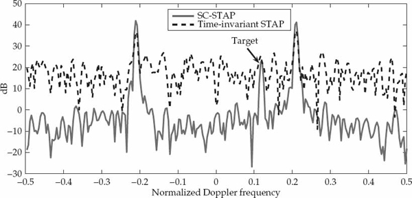
FIGURE 11.8 Doppler spectra for the operational time-invariant STAP and SC-STAP routines in the ship detection example with an injected useful signal. © Commonwealth of Australia 2011.
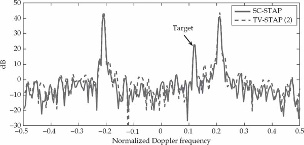
FIGURE 11.9 Doppler spectra for the operational SC-STAP and TV-STAP routines in the ship detection example with an injected useful signal. © Commonwealth of Australia 2011.
Figure 11.8 illustrates the output of the operational SC-STAP filter ŵk(t), which can detect a synthetic target 30 dB above the local background disturbance level. In contrast, the time-invariant STAP filter ŵ was not able to distinguish this useful signal due to masking from inadequately rejected hot clutter. Figure 11.9 compares the performance of SC-STAP and TV-STAP using a batch length of Np = 2 PRIs. The curves indicate quite similar performance, which confirms that TV-STAP can offer a useful computational advantage for negligible performance loss in the simulated ship-detection example.
Now consider the high PRF (air-detection) scenario, with terrain-scattered cold clutter. In this case, the PRI has one-tenth of the duration assumed for the previous (ship-detection) simulation. The inter-PRI temporal correlation coefficients of the hot-clutter modes may be adjusted to account for the higher PRF of fp = 50 Hz in accordance with the decaying exponential model 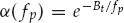 where the bandwidth Bt is computed from the hot-clutter parameters listed for the low PRF mode (fp = 5 Hz) in Table 11.2. This procedure is used to adjust the hot-clutter coefficients αml for the fp = 50 Hz case in Table 11.2. The first-order AR model is adopted to describe terrain-scattered cold clutter using the parameters listed in Table 11.3.
Figures 11.10 and 11.11 show the Doppler spectra resulting for operational STAP schemes in the high PRF example. In this case, both SC-STAP and TV-STAP employ a single auxiliary linear constraint to protect SCV, which is appropriate for the assumed first-order AR cold-clutter model. It is clear from Figure 11.10 that time-invariant STAP leads to a degradation in hot clutter rejection of about 20 dB relative to SC-STAP. This degradation is severe enough to mask the useful signal, which is readily detected by SC-STAP in Figure 11.10. Figure 11.11 compares SC-STAP with TV-STAP using a batch length of Np = 16 pulses. This batch length provides an order of magnitude reduction in computational load with respect to SC-STAP for negligible loss in hot-clutter rejection. Clearly, both SC-STAP and TV-STAP detect the useful signal in Figure 11.11.
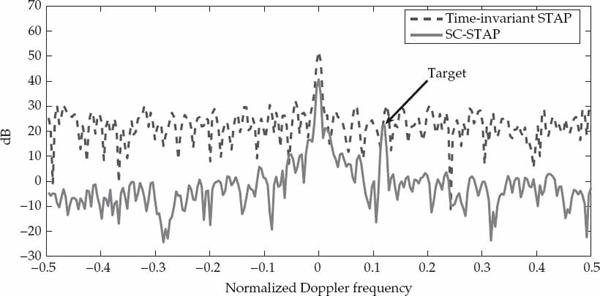
FIGURE 11.10 Doppler spectra for operational time-invariant STAP and SC-STAP routines in the aircraft detection example with an injected target. © Commonwealth of Australia 2011.
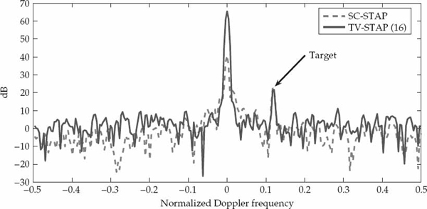
FIGURE 11.11 Doppler spectra for operational SC-STAP and TV-STAP routines in the aircraft detection example with an injected target. © Commonwealth of Australia 2011.
11.4 Post-Doppler STAP Implementation
In the previous section, fast-time STAP was used to mitigate hot clutter signals that were time-continuous over the CPI, broadband with respect to the sampling rate, incoherent with the radar waveform, and received as multiple propagation modes, one or more of which may enter through the main lobe of the radar beam. The correlation properties of these active interferences were assumed to be statistically homogeneous in fast-time, which allowed STAP filters to be trained effectively using secondary data obtained from a limited number range bins free of cold clutter in each repetition period. Unwanted signals from passive sources that reflect or scatter the radar signal, as opposed to radiating an independent waveform, give rise to coherent disturbances, which pose a quite different problem as far as mitigation by means of STAP is concerned.
For example, radar echoes from meteor trails, or highly dynamic electron-density irregularities in the ionosphere, may produce echoes that are significantly spread in Doppler. Such returns have the potential to mask useful signals over much of the target velocity search space. Perhaps more importantly, these coherent disturbance signals tend to have spatial characteristics that are highly heterogeneous in range. This is because the energy of a coherent signal received from a particular scatterer is localized in range after pulse compression. In general, this means that each range cell samples a different spatial distribution of scatterers. The main implication of such heterogeneity is that adaptive filters need to be trained on one range cell at a time. In this case, secondary data is taken from slow-time samples or Doppler bins in the range cell under test.
In the previous chapter, a post-Doppler SAP method with range-dependent weights was described. When main-beam interference from active sources is additionally present, this scheme will attempt to jointly cancel the coherent disturbance and main-beam interference, which typically leads to performance degradation. Moreover, the main-beam interference may be received via a single dominant mode instead of multiple propagation paths. In this case, fast-time STAP is not effective for broadband sources as it relies on multipath to cancel the main-beam interference. However, if the main-beam interference has an effective bandwidth that is small compared to the radar bandwidth, the significant correlation existing between fast-time samples (acquired at the Nyquist rate fs) can be exploited for cancelation. Typically, narrowband interference in the HF band has an effective bandwidth that is higher than the pulse repetition frequency fp, so its energy spreads across Doppler. Narrowband interference therefore has the potential to mask targets in all range-Doppler cells.
In this section, a post-Doppler STAP approach is described for jointly mitigating range-heterogeneous spread-Doppler clutter and main-beam narrowband (i.e., range-correlated) interference. The proposed architecture simultaneously processes radar data across a number of auxiliary beams and ranges. The former provides spatial DOFs for canceling sidelobe signals, while the latter provides fast-time DOFs for canceling main-beam interference that is correlated in range. An important point is that training of the STAP filter is performed on a range-by-range basis in the Doppler domain for the reasons stated above. Another key point is that the use of a fast-time tap delay line behind each spatial DOF is dispensed with in this application. An alternative reduced-dimension post-Doppler STAP architecture in which the number of spatial and temporal DOFs add instead of multiply will be proposed in Section 11.4.1. Experimental results are illustrated for a real-time practical implementation of this alternative STAP architecture. These results demonstrate the performance of an operational routine in a trial involving a cooperative aircraft target where on-board GPS data is used to provide ground-truth on the flight path.
11.4.1 Algorithm Description
Some of the symbols used in the first part of this chapter will be redefined in this section to avoid cumbersome notation. In traditional STAP architectures, the use of K spatial channels (receivers or beams) and L temporal taps (fast-time samples in this case) results in a space-time filter dimension equal to the product K × L. Even for modest parameter values, e.g., K = 16 and L = 8, this architecture results in a processor with K × L = 128 DOFs. The problem with such a large filter dimension is that adaptation on a range-by-range basis needs to be achieved by training over Doppler bins, which are typically limited to P = 256 or less in practical OTH radar applications. Moreover, the effective number of independent Doppler bins is usually about half this amount due to the low sidelobe windows often used for Doppler processing.
To counter the finite sample-support problem, rank reduction based on singular value decomposition may be performed on the data, but such procedures are computationally expensive to apply for each range cell. Diagonal loading provides an alternative to improve convergence rate, but the processor dimension and hence computational load is not reduced. A different option is to identify a reduced dimension post-Doppler STAP architecture to address the practical issues of finite sample support and computational load.
This section describes an alternative post-Doppler STAP formulation that uses K beams for spatial adaptation and L fast-time taps for temporal adaptation with the latter taken only from the reference beam. In this way, the STAP filter dimension is given by the sum Q = K + L, which is typically much less than the product Q KL. The main benefits of this architecture include reduced demands on statistically homogeneous training data and lower computational load for real-time implementation.
Figure 11.12 illustrates the reduced-dimension STAP processing architecture using K + L degrees of freedom. In our previous example, where K = 16 and L = 8, we have Q = 24. This is a significant reduction on K × L = 128. In addition, Q > 5P for P = 128 Doppler cells, which means that sufficient training is available for range-by-range adaptation. In this architecture, the main and auxiliary beams are formed conventionally. The weighted combination of auxiliary beam outputs provides a means to cancel sidelobe disturbances. This includes unwanted (sidelobe) signals from coherent and incoherent sources.
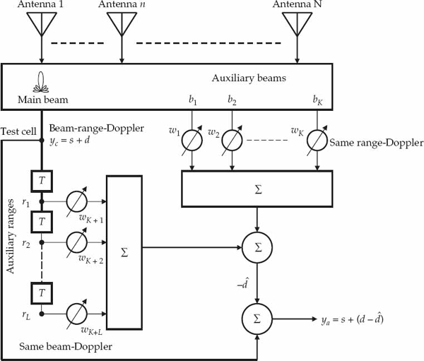
FIGURE 11.12 Reduced-dimension STAP processing scheme with K spatial taps (auxiliary beams) and L temporal taps (auxiliary ranges) that results in a processor dimension of K + L instead of K × L (degrees of freedom). © Commonwealth of Australia 2011.
On the other hand, the fast-time taps behind the main beam output provide a means to reject range-correlated interference that may be received from the useful signal direction. This may include interference from transient (impulsive) signals, or long-lived (narrowband) signals on the scale of the CPI. Naturally, impulsive interference that corrupts only a few PRIs can also be mitigated by excision and linear prediction techniques applied in the slow-time domain. However, exploiting the range-correlation structure of such interferences can have advantages when a significant number of PRIs in the CPI are affected.
As the spatial and temporal taps in this STAP architecture are used to mitigate different interference types, it can be argued that a factored approach involving SAP followed by range-only adaptive processing (RAP), or vice versa, could be applied to further reduce sample-support requirements and computational load. The main issue is that supervised training data containing only one interference type in isolation from the other is generally not available for the described application. For example, the presence of main-beam interference in the SAP training data can bias the filter weights needed to cancel sidelobe disturbances, as well as distort the main lobe of the antenna pattern. In such cases, STAP provides an avenue for joint cancelation based on training data that contains a mixture of the different disturbance types.
However, turning the STAP architecture of Figure 11.12 into a robust and practical technique requires a number of significant technical challenges to be overcome. Performance-related aspects include: (1) the quality of disturbance suppression, which depends on the allocation and relative distribution of adaptive DOFs in space and time, as well as the training-data selection strategy, and (2) the impact on useful signals, where it is important to avoid target echo self-cancelation and copying effects that can produce false alarms or degrade parameter estimation accuracy for target tracking.
Robustness to the wide diversity of operational conditions encountered by practical OTH radar systems in the unpredictable HF environment is also essential. All of these prerequisites need to be achieved with minimal or no requirement for human intervention, while the algorithm needs to be computationally efficient to permit real-time operation on existing platforms without severely consuming radar resources. Satisfying this combination of inter-dependent objectives is typically not straightforward, but necessary in order to claim an effective real-time STAP capability. At this point, the proposed post-Doppler STAP method, referred to as range-dependent (RD)-STAP, is described.
Let the N-dimensional complex vector x = [x1, x2, …, xN]T be the element-space spatial snapshot resulting at a particular range-Doppler cell after matched filtering is performed in each receiver. For a two-dimensional array, the radar look direction is defined by steering angles in azimuth θo and elevation φo. The conventional beamformer output for the main beam steered in this direction is given by the complex scalar yc = s†(θo, φo)x, where s†(θo, φo) is the array steering vector.
The array steering vector is parametrically defined by Eqn. (11.69), where the term  is the signal wave vector, and rn = [xn, yn, zn]T is the antenna position vector in Cartesian coordinates relative to the phase reference for the elements n = 1, 2, …, N. Conventional beamforming of each range-Doppler cell processed by the system over a set of beams steered in different directions that (at least) cover the surveillance region, results in a beam-range-Doppler (BRD) data cube. In other words, the raw data cube with dimensions of antenna element, fast-time and slow-time is transformed by conventional processing to a data cube with dimensions of steer direction, range cell, and Doppler bin. This conventionally processed data cube is normally passed on for CFAR processing followed by peak detection-estimation and tracking.
(11.69)
The proposed RD-STAP method is applied directly to the conventional BRD data cube, and may therefore be “switched in” as the final stage of the signal-processing chain, i.e., immediately prior to the CFAR processing step. A well-designed STAP procedure is able to substantially improve detection performance when interference is present, but should automatically revert back to what is effectively conventional processing under quiescent conditions. In this case, a radar operator can keep STAP operating all the time, providing the computational burden is low enough so as not to compromise other radar functions or performance. In essence, the purpose of RD-STAP is to remove residual interference that contaminates the conventionally processed BRD map before this data is passed on for subsequent CFAR processing.
Define z ∈ CK+L in Eqn. (11.70) as the primary data vector to be processed by the STAP filter. The first scalar element of this data vector yc is the conventional output at a particular (unnamed) location in the BRD data cube. The RD-STAP procedure assigns each cell in the BRD map as the current test cell in turn. The second component of the primary data vector contains a set of K auxiliary beam outputs, contained in the vector b = [b1, b2, …, bK]T, where each auxiliary beam sample bk is extracted from the same range-Doppler coordinate as the test cell yc, but from an auxiliary beam steered in a different direction to the main beam. The third component of z contains a set of L auxiliary range cells denoted by r = [r1, r2, …, rL]T, where each fast-time sample r is taken from the same beam-Doppler coordinate as the test cell yc, but from a fast-time sample different to the current range.
(11.70)
Figure 11.12 illustrates the conventional beam-range-Doppler sample yc, the L range samples r1, …, rL from the same beam and Doppler cell as yc, and the K auxiliary beams b1, …, bL from the same range and Doppler cell as yc. Naturally, the useful signal vector needs to be modified in accordance with the beam and range transformations to reflect the chosen set of auxiliary spatial channels and range taps in the primary data vector z.
Let Tb be the K × N matrix that transforms the N receiver outputs to the K selected auxiliary beams, such that b = Tbx. For example, if the K selected auxiliary beams are conventionally formed in steer directions  , the transformation matrix would be defined as Tb = [s(θ1, φ1), …, s(θK, φK)]†. If the auxiliary beams are formed using a taper function
  to lower the antenna pattern sidelobes, the transformation matrix becomes Tb = [t(θ1, φ1), …, t(θK, φK)]†, where t(θk, φk) = Ds(θk, φk) and D = diag[w1, …, wn]. In any case, the spatial transformation of the steering vector is given by
(11.71)
Similarly, define Tr as the L × M matrix that transforms the M fast-time samples in the PRI to the L selected auxiliary range cells. For a CW-OTH radar system, each row of Tr = [g(τ1), …, g(τL)]† is an M-dimensional vector g†(τ) that contains the matched filter coefficients used for pulse compression, i.e., to form the range bin at fast-time sample delay τ. Typically, the elements of g(τ) correspond to the transmitted radar waveform delayed by τ fast-time samples and shaded in amplitude to reduce range sidelobes. For a PW-OTH radar system, where fast-time samples correspond directly to range bins, g(τ) may be considered a vector with a unit element in position and zeros elsewhere. The modification to the temporal component of the steering vector is given by Eqn. (11.72), where g(τo) is the radar waveform with delay τo corresponding to the range bin of the current output yc.
(11.72)
The space-time steering vector for the proposed RD-STAP architecture may then be constructed as v in Eqn. (11.73). Note that v involves a concatenation of the transformed spatial and temporal steering vectors rather than a Kronecker product. Stated simply, v is the useful signal vector for the proposed STAP architecture. This vector represents the space-time signature of the target echo that is sought in the primary data z. When a detection results, target presence is declared at the beam-range-Doppler coordinates of the test sample yc. Note that the signal vector v is valid for all Doppler frequency bins, and only changes when different auxiliary beams or ranges are selected. The vectors vb and vr effectively reduce to zero when the beam and range (sidelobe) responses to the target echo fall below the thermal noise floor in the selected auxiliary beams and ranges, respectively. In this case, any useful signal energy leaking into the auxiliary beams and ranges is small enough to be neglected.
(11.73)
When such conditions do not hold, either because of the coordinates of the selected auxiliary beams or ranges relative to the test cell, or the manner in which the auxiliary beams and ranges are formed (with due regard to the strength of the useful signal), the vectors vb and vr will contain significant nonzero elements. In this case, it is advisable to normalize the useful signal signature vector, such that it has fixed unit norm v†v = 1. If the statistically expected covariance matrix R = E{zzH|H0} for the primary data vector were known under the null hypothesis (i.e., the disturbance-only covariance matrix), the optimal STAP weight vector wopt for processing the data vector would be given by the well-known rule in Eqn. (11.74).
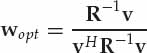
(11.74)
In practice, this matrix is not known a priori and must be estimated from a set of D secondary data vectors zd indexed by d = 1, 2, …, D. These secondary vectors are assumed to be free of the useful signal and to share the same statistical characteristics as the disturbance in the primary data z. In the current application, the disturbance statistics are presumed to be heterogeneous in range. For this reason, the secondary data is extracted from P Doppler bins available in the same range cell as the sample under test. The set of D < P Doppler bins utilized for training typically exclude the test cell plus a guard cell either side of it. Doppler bins deemed to contain “outliers” are also screened out from the training set. A disturbance sample covariance matrix with appropriate regularization is formed using the selected secondary data, as in Eqn. (11.75). The operational STAP
weights ŵ are then computed by replacing the unknown true covariance matrix R in Eqn. (11.74) with its estimate in Eqn. (11.75).

(11.75)
The test and guard cells are excluded from the training data to avoid attenuation of target echoes. These echoes are assumed to have a steady Doppler shift over the CPI, such that significant useful signal energy is not present outside of the guard cells. On the other hand, disturbances such as ionospheric clutter and incoherent interference are often more spread in Doppler than target echoes and will therefore be captured in the training data. The resulting adaptive filter is applied to the primary data to obtain the RD-STAP output ya given by Eqn. (11.76). This output may be directly compared with the conventional output yc.
(11.76)
At this point, a number of questions arise. First, how are the number and coordinates of auxiliary beams and ranges chosen? Second, how are number and coordinates of the Doppler training bins selected for a particular test cell? These decisions need to strike a balance between performance and computational complexity. As far as convergence rate for the sample matrix inverse (SMI) technique is concerned, it is recommended that the number of independent training vectors is at least twice the STAP filter dimension (Reed, Mallet, and Brennan 1974). This rule of thumb is expressed in Eqn. (11.77). Given that adjacent Doppler cells are not strictly independent due to the window used for controlling spectral leakage, the requirement D > 4Q may be more appropriate if neighboring Doppler bins are used and regularization is not applied. Appropriate diagonal loading can under certain circumstances significantly reduce the number of independent samples required (Cheremisin 1982). In general, the choice of processor DOFs Q should ensure that sufficient training data is available for adaptation given the number of Doppler bins is limited to P.
(11.77)
From a computational perspective, updating the STAP weights every Doppler cell may be prohibitive. The matrix inversion lemma (Woodbury’s identity) can be used to reduce computational load for low-rank updates of the covariance matrix, but a much faster method is to process a set of Doppler cells using a single weight vector. Similar to the purely spatial approach described in the previous chapter, the positive and negative Doppler frequency bins are processed by independent STAP filters. This requires two matrix inversions of dimension Q + 1 for processing all Doppler bins in a beam-range resolution cell. While this approach clearly avoids target contamination in the training data, the number of training cells available for each estimate is half the total number of Doppler bins minus the number of outliers.
The outliers are excluded from the training data because their statistical characteristics are deemed to be not sufficiently representative of the disturbance to be mitigated. In this application, outliers are mainly due to powerful surface clutter components concentrated near zero Doppler frequency, as well as Doppler-shifted target-like returns. For a training data volume of at least four times the STAP filter dimension (F = 4), the described rationale imposes an upper limit on the value of Q given by Eqn. (11.78), where J is the maximum number of discarded outlier samples in the positive or negative half of the Doppler spectrum, and  denotes integer truncation (the floor function).
(11.78)
This may be interpreted as an upper limit on Q based on adaptive filter performance considerations. As computational load grows with Q, the upper limit on the value of Q for real-time processing may be lower than that of Eqn. (11.78). Hence, Q is selected as the highest value that satisfies the finite sample-support constraints in Eqn. (11.78), and the restrictions on real-time processing capacity. The processing load may be reduced if the set of beams and ranges contained in the data vector z remains the same as the sample under test changes, i.e., when one of the auxiliary cells is interchanged with the sample under test and vice versa without introducing new beams or ranges in z. It is then possible to process a block of K + 1 beams and L + 1 ranges with no further matrix inversions simply by modifying the useful signal signature vector to reflect the new position of the current sample under test.
For example, if the previous test cell becomes the first auxiliary beam and vice versa, the signal vector may be changed to Eqn. (11.79), where unity defines the current position of the main beam and the elements bk are calculated accordingly. The resulting signal vector is normalized to v†v = 1, as before. The weights are then computed by substituting the new signal vector into Eqn. (11.75) with the same matrix inverse for either the positive or negative Doppler bins. An analogous modification is made when swapping one of the auxiliary range cells for the sample under test. Significant computational savings can be achieved when a fixed set of beams and ranges are processed as a block in this manner. The compromise here is that the choice of auxiliary beams and ranges cannot be tailored to specifically suit the test cells on an individual basis.
(11.79)
Once Q is selected based on the aforementioned considerations, the next issue relates to the allocation of DOFs among spatial channels and fast-time taps, as well as the selection of specific auxiliary beams and ranges from the conventional BRD data cube. The latter requires a method for preferentially ranking the auxiliary beams and ranges. A reasonable approach is to rank auxiliary beams according to an estimate of the received disturbance power. For example, the median value of the Doppler spectrum may be used to provide a robust measure of disturbance level. Auxiliary beams with higher disturbance levels are chosen in preference to those containing lower power. On the other hand, the auxiliary ranges are selected in the immediate neighborhood of the test range, since the disturbance in these “local” cells is likely to be more highly correlated with that in the test cell. Such criteria may be used to pick the auxiliary beams and ranges once K and L are specified from the value of Q.
The partitioning of Q into K spatial channels and L fast-time taps is a more complex issue, as it depends on the prevailing correlation properties of the disturbance relative to the structure of the useful signal vector. This issue was investigated in Holdsworth and Fabrizio (2008). A reasonable starting point is to calculate the relative disturbance cancelation ratio using spatial and temporal DOF for adaptation separately. The relative gains may be compared and the values of K and L allocated based on an estimate of the relative benefits from adaptation in each dimension. An optimum strategy has not been developed excluding the brute force analysis of all possible combinations. This aspect merits further study. In practice, some degree of experimentation may be required to empirically derive suitable rules for determining the values of K and L for a given Q.
Once the RD-STAP system dimensions are selected, a reliable method for identifying outlier cells in each half of Doppler space is required. A preliminary step involves identifying the Doppler bins occupied by relatively strong surface clutter typically near zero Doppler frequency. Once the edges defining the clutter Doppler band to be excluded have been determined, an initial SCM may be formed using all remaining Doppler bins. A non-homogeneity detector based on the Generalized Inner Product (GIP) can then be applied to identify the presence of outliers in the training data. A small but fixed percentage of samples with the highest level of heterogeneity may then be discarded from the final covariance matrix estimates used to derive the RD-STAP filters for each half of Doppler space. This ensures a that known number of snapshots remain for training, while reducing the influence of the strongest outliers that could potentially bias the filter estimate.
In summary, the algorithm may be broken down into three main steps: (1) select the total number of DOFs Q to be allocated for adaptive processing, (2) partition the available DOFs into K spatial channels and L temporal taps and select these from the conventional BRD data cube based on a ranking system, and (3) apply the training-data selection strategy to estimate the RD-STAP filters for each resolution cell in the radar coverage. When the rules for these three main procedures are established and automatically implemented, the STAP algorithm is essentially self-configuring with no need for human intervention.
11.4.2 Experimental Results
The experimental data analyzed in this study were collected between 04:45 and 05:15 UT on 17 April 2004 using a two-dimensional (L-shaped) antenna array located near Darwin in Northern Australia. The array consisted of 16 vertically polarized “whip” antenna elements with 8 elements on each arm uniformly spaced 8 m apart (a dummy element was included at the end of each arm to avoid mutual coupling). The output of each antenna element was connected to an individual HF receiver. The main features of the receiving system have been discussed in the previous chapter. An OTH radar transmitter located approximately 1850 km to the south-east of Darwin illuminated the region around the receiver via the ionosphere. This allowed the forward-based receiver array to acquire echoes from targets in the line of sight via a direct path.
The radar signal was a linear frequency modulated continuous waveform (FMCW) with carrier frequency fc = 19.380 MHz, bandwidth fb = 20 kHz, and pulse repetition frequency fp = 62.5 Hz. The coherent integration time (CIT) consisted of P = 248 PRIs and was approximately 4 seconds long. An HF spectrum analyzer was used to monitor channel occupancy and indicated that the carrier frequency was clear of other users at the time of the experiment. The trial involved a cooperative Learjet aircraft target (see Fig 10.22) that was chartered to fly out from Darwin in a north-west direction to a range of approximately 400 km at a cruising altitude of about 31000 ft.
GPS logging equipment on board the aircraft enabled the target’s range, bearing, and bi-static Doppler shift to be determined during the flight. At predetermined locations, the aircraft performed a 360 degree turn to clearly distinguish its echo from other echoes on the radar display by virtue of its unique Doppler-time signature. Range and Doppler profiles of the flight path derived from on-board GPS data logs appear in Figures 11.13 and 11.14 over the 15-minute period of interest (04:25–04:40 UT). During this time, a 360-degree maneuver commenced at about 04:29 UT. The maneuver is quite noticeable in the range and Doppler versus time profiles.
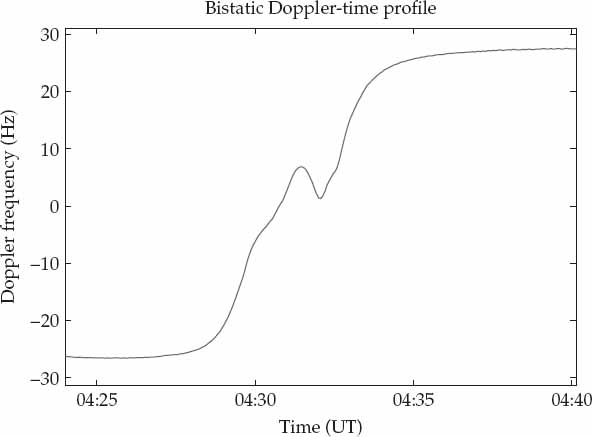
FIGURE 11.13 Bistatic Doppler-time profile of the aircraft target flight path computed from the GPS data. © Commonwealth of Australia 2011.
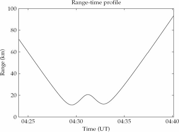
FIGURE 11.14 Range-time profile of the aircraft target flight-path (relative to the LOS receiver) computed from the GPS data. © Commonwealth of Australia 2011.
11.4.2.1 Range-Doppler Displays
The target maneuver occurs when the echo is in range cells contaminated by relatively strong spread-Doppler clutter and occasionally strong RFI that affects the main beam but is correlated in range. Figure 11.15 shows a range-Doppler map for a conventional beam steered in the target direction. The azimuth and elevation of the target were determined from the known position of the aircraft (using GPS data) at the time when this CPI was recorded. In this display, range bins are ordered vertically with the nearest range at the bottom. This CPI is representative of the data collected during intervals deemed to be free of strong RFI.
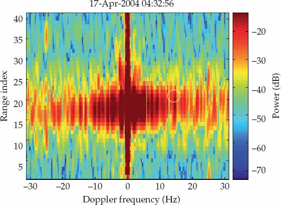
In addition to the main clutter “ridge,” which is apparent in all ranges near zero Doppler frequency, spread-Doppler clutter is also present and contributes to raising the disturbance level over the entire velocity search space in a band of range bins with indices roughly between 10 and 25. The expected target position in radar coordinates calculated from the GPS data is circled on this display at about 14 Hz Doppler frequency and near range bin 21. However, conventional processing cannot clearly distinguish the faint target echo, which is masked by the more powerful spread-Doppler clutter in this CPI.
The proposed RD-STAP technique was implemented with K = 8 auxiliary beams and L = 4 auxiliary ranges. The auxiliary beams were steered at the same elevation as the main beam and equally spaced 10 degrees apart in azimuth, such that four beams were formed either side of the main beam. Once the clutter-contaminated Doppler bins near 0 Hz and the outliers were removed from the training data, the number of samples remaining in the positive and negative halves of Doppler space was D = 96. For Q = K + L = 12, this corresponds to D = 8Q. Figure 11.16 shows the RD-STAP output for the same data as Figure 11.15. The offending spread-Doppler clutter has been effectively removed and the target can be easily detected at the expected location.
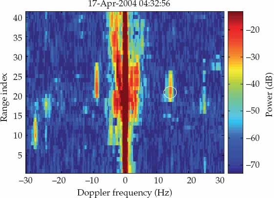
In identical format, Figures 11.17 and 11.18 show the conventional and RD-STAP results for a CPI recorded 7 minutes later, when the target had moved out of the spread-Doppler clutter affected ranges, but was masked by strong RFI from an unknown source. This source was received within the main beam and effectively precluded target detection over practically all range-Doppler bins when conventional processing was applied. Figure 11.17 indicates that the RFI exhibits significant structure in range, which may be exploited for cancelation. Indeed, Figure 11.18 shows that STAP cancels the RFI and clearly detects the target at the expected location near range bin 22 with a Doppler shift of about 28 Hz. A potential target of opportunity is also distinguished near range bin 15 at a Doppler shift of about 19 Hz, but this candidate is unconfirmed and will not be considered further.
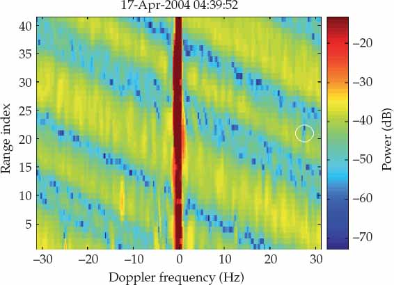
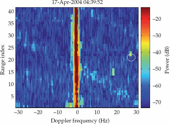
11.4.2.2 Doppler-Time Signature
A synoptic view of performance over a collection of CPIs is most effectively shown as the time-evolution of Doppler spectra resulting in the target beam-range cell. Displays of this kind are sometimes referred to as waterfall or scroll displays. Since the target migrates to different range and beam coordinates over time, the waterfall display is populated only with Doppler spectra corresponding to the radar spatial resolution cell known to contain the target at the time of the CPI. GPS data were used to determine the range-beam cell containing the target for each CPI processed, such that the appropriate Doppler spectrum could be extracted. Figures 11.19 and 11.20 show the waterfall displays for conventional processing and RD-STAP, respectively.
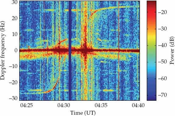

The 360-degree turn results in a passage of the target trace from one side of Doppler space to the another. Since this occurs at a time when the target range coincides with that of the spread-Doppler clutter, the target maneuver is not clearly observed in the conventionally processed output of Figure 11.19. On the other hand, Figure 11.20 shows that RD-STAP effectively and consistently removes the spread-Doppler clutter to make the target maneuver clearly visible. The RD-STAP waterfall display in Figure 11.20 reveals a sharp and continuous Doppler-time target signature that agrees remarkably well with the Doppler-time profile predicted from the GPS data in Figure 11.13. Before and after the target maneuver (i.e., toward the left and right extremities of the waterfall display), the echo has an essentially “steady-state” bistatic Doppler shift of around ±28 Hz.
In these intensity-modulated displays, the Doppler spectrum is plotted vertically, with a single-line spectrum being shown per CPI. The Doppler spectra from successive CPI are stacked next to one another horizontally as a function of the CPI start time. The 15 minutes of data analyzed to produce these displays contains more than 200 CPI. The powerful horizontal clutter trace near zero Doppler frequency is clearly evident in both displays. As the target initially moves toward the radar in range, it enters the spread-Doppler clutter effected region around 04:32 UT. At this time, the disturbance commences to obscure the Doppler-time profile of the target maneuver in Figure 11.19. An example of such obscuration is shown in the conventional range-Doppler display of Figure 11.15.
In these sections of the flight path the target range is not within the spread-Doppler clutter effected region and conventional processing performs rather well except for the occasional CPI contaminated by strong RFI, as shown in Figure 11.17 for example. RD-SAP is seen to remove the interference due to these sporadic events, as illustrated by Figure 11.18. In this data set, the RD-STAP technique is shown to provide the radar system with greater immunity against spread-Doppler clutter and RFI that is correlated in range. The former is particularly relevant for detection at ranges close to the direct-wave clutter, while latter may be important in operational situations where a frequency change is not practical at a critical time in the mission and the presence of persistent range-correlated RFI threatens to preclude target detection across all range-Doppler cells over many CPIs.
11.4.3 Discussion
The first section of this chapter discussed three different STAP architectures referred to as slow-time STAP, fast-time STAP, and 3D-STAP. The disturbance characteristics motivating each STAP architecture were briefly identified in the context of both airborne microwave radar and HF OTH radar. It was argued that fast-time STAP is applicable in OTH radar for the problem of hot clutter mitigation, while slow-time STAP for cold clutter mitigation is not as well motivated for OTH radar as it is for airborne radar. In unsupervised training scenarios, 3D-STAP for joint hot- and cold-clutter mitigation may have applications for OTH radar, but practical issues such as finite sample support and computational complexity generally become more difficult to overcome for such schemes. For these reasons, only fast-time STAP was considered further and appropriate data models were developed in the second section of this chapter.
Fast-time STAP offers two important advantages with respect to spatial adaptive processing (SAP). The first situation of practical interest arises when the number of diffusely scattered hot clutter paths summed over the number of independent sources exceeds the number of antenna elements or spatial channels. In this case, SAP is exhausted of degrees of freedom and cannot effectively cancel the composite disturbance. Fast-time STAP provides a means to extend the number of adaptive DOFs beyond the rank of the hot clutter subspace and is therefore potentially able to cancel the composite disturbance more effectively than SAP. Second, SAP is not suitable for canceling disturbances received in the main-beam, as effective rejection often comes at the expense of significant main-beam distortion in this scae. Fast-time STAP is able to exploit multipath scattering from different angles to provide immunity against main-beam disturbance components. In the absence of multipath, fast-time STAP can also exploit range correlation to cancel main-beam interference in the special case of narrowband interference or impulsive noise sources.
In the general case of broadband interference sources, the non-stationarity of the hot-clutter covariance matrix over the relatively long (OTH radar) CPI creates a problem for standard fast-time STAP procedures. Specifically, the standard approach based on a fast-time STAP filter that is held fixed over the CPI fails to effectively reject the hot clutter because the integrated covariance matrix (averaged over the whole CPI) typically has full rank as a consequence of the non-stationarity hot-clutter propagation paths. On the other hand, the standard approach based on a time-varying weight vector that changes from one PRI to another can effectively reject non-stationary hot clutter, but typically has a devastating effect on sub-clutter visibility, as such filters destroy the slow-time correlation properties of the processed cold-clutter output.
In the third section of this chapter, two alternative fast-time STAP techniques were described to mitigate hot-clutter non-stationarity over the CPI, while simultaneously preserving the Doppler spectrum characteristics of the output cold-clutter signal. The SC-STAP method updates the weight vector every PRI but employs auxiliary linear stochastic constraints to stabilize the auto-regressive characteristics of the output cold-clutter signal. Motivated by the need to reduce computational load for practical implementation in real-time operational systems, the TV-STAP algorithm was subsequently introduced.
By updating the weight vector at a rate commensurate with the prevailing rate of hot-clutter non-stationarity, simulations demonstrated that TV-STAP can achieve computational advantages relative to SC-STAP while yielding similar performance to the SC-STAP method. Importantly, it was also shown that TV-STAP can protect the cold-clutter Doppler spectrum when it is described by a scalar-type AR process. Indeed, the TV-STAP algorithm reverts back to the SC-STAP technique as a special case for a particular choice of algorithm parameters. As such, TV-SAP may be viewed as a generalization of the SC-STAP technique that provides scope to jointly optimize performance and computational load.
The mitigation of disturbance signals coherent with the radar waveform via STAP was considered in the final section of this chapter. Such signals can have statistical characteristics that are significantly heterogeneous in range. In this case, effective mitigation requires the adaptive filter to be updated on a range-by-range basis.
A post-Doppler and beam-space fast-time STAP architecture for the joint cancelation of sidelobe spread-Doppler clutter and range-correlated interference (potentially received in the main beam) was described and tested in the final section. A peculiarity of this reduced-dimension RD-STAP technique is that the adaptive filter dimension is the sum rather than the product of the number of spatial and temporal DOFs. This enables the processor to cope well with low sample support and keep the computational load to modest levels for real-time implementation. Both aspects are of prime importance and must be adequately addressed for operational systems.
The performance of the proposed RD-STAP method, which is capable of running in real-time on contemporary computing platforms, was demonstrated and compared against conventional processing using over 200 CPIs of experimental data. The advantages provided by this STAP architecture relative to conventional processing were observed in cases where spread-Doppler clutter and intermittent RFI masked echoes from a cooperative (Learjet) aircraft target. STAP clearly revealed the Doppler-time signature of the cooperative target during a 360-degree turn maneuver, which was not easily visible at the conventional processing output. The target trace seen at the STAP output agreed remarkably well with the flight path predictions derived from GPS data recorded on-board the cooperative aircraft.
____________________
1 This is often the case for a relatively quiet mid-latitude ionosphere. However, in auroral regions, e.g., the occurrence of high plasma drift velocities due to convection can lead to appreciable DOA-Doppler coupling on the scattered skywave signals. In this case, the radar platform is stationary but the propagation medium is moving.
2 In slow-moving target detection applications, angle-Doppler coupling effects can become more significant in OTH radar as useful signals are often located close to the main clutter “ridge.”
..................Content has been hidden....................
You can't read the all page of ebook, please click here login for view all page.