
CHAPTER 6
Wave-Interference Model
A wide variety of high-frequency (HF) systems rely on the ionosphere as a radio wave propagation medium for operation over long distances well beyond the line-of-sight. Examples include HF communication links for transferring data or speech between remote sites, direction-finding networks for locating the position of distant HF emitters, and OTH radars used for early-warning wide-area surveillance. In practice, the performance of HF systems utilizing the ionosphere not only depends on the choice of operating parameters, but also on the characteristics of the propagation medium. For this reason, there is great interest in analyzing and modeling the properties of HF signals reflected by the ionosphere, particularly those which can potentially limit system performance.
A popular model for skywave HF signals received by antenna arrays consists of a superposition of multiple plane waves that emanate from the different ionospheric reflection points. Specifically, the traditional signal-processing model assumes that a single specularly reflected plane wave component is received for each distinct propagation mode. This model is rather simple, far too simple in fact to satisfactorily describe the actual signal structure received by practical HF arrays. Typically, HF signals undergo diffuse scattering from a number of spatially extended but often localized regions in the ionosphere. A question that frequently arises is whether the complex fading of the received signals can be decomposed as the sum of a relatively small number of plane wave components with slightly different directions-of-arrival and Doppler shifts, such that the fading pattern observed on the ground can be represented accurately by the interference of these waves over a limited period of time.
The main objective of this chapter is to quantitatively assess the virtues and limitations of the wave interference model for describing the observed signal fading phenomena in space and time. Section 6.1 discusses the applications of the wave interference model in different contexts and defines the scope of this model for the purpose of this chapter. Section 6.2 describes a multichannel scattering function experiment to demonstrate the existence and time-varying characteristics of wavefront distortions for resolved ionospheric modes received on a very wide aperture antenna array. Section 6.3 mathematically describes the wave-interference model and a super-resolution parameter estimation technique for the identification of closely spaced component rays. A fitting accuracy measure is also described in this section to assess the performance of the wave-interference model using real data. Section 6.4 presents an extended set of experimental results to illustrate the domain of applicability and shortcomings of the wave interference model for a relatively quiet mid-latitude ionospheric channel.
6.1 Deterministic Description
Compensation for performance degradations incurred as a result of propagation effects, which can significantly distort the received signal structure relative to that expected under ideal or benign conditions, is often sought in the form of ameliorative signal processing. Modern signal-processing algorithms are usually designed and optimized on the basis of mathematical models that are presumed to reflect the characteristics of actual signals received in practice, either deterministically or in a statistical sense. Not surprisingly, the effectiveness of model-based algorithms in real-world systems is largely determined by the fidelity with which the assumed model is able to represent the properties of the acquired data. Importantly, modern systems capable of sensing fine scale features of the received signal structure require models of commensurate sophistication and accuracy to appropriately guide signal processor design.
The models which have traditionally been used as bases for the development of many conventional signal-processing techniques have been rather simple, particularly for state-of-the-art HF systems such as OTH radar, where signals are sampled by very well calibrated wide aperture antenna arrays using receivers with high spectral purity and dynamic range. In a number of important signal-processing applications, traditional models do not provide a sufficiently realistic description of the received signals. At the moment, an important frontier in OTH radar development lies in the area of improving the received signal models and developing more advanced signal-processing techniques based on these improved models to enhance system performance.
HF propagation models derived from consideration of detailed ionospheric physics provide valuable phenomenological insights and can potentially yield high quality representations of the received signal structure. However, the physical parameters these models depend upon are generally not known with a high degree of certainty, and in many cases, the mathematical formulations are quite detailed and not always tractable for the purpose of designing and optimizing real-time signal-processing algorithms. These factors can restrict their utility in a number of practical applications, particularly when the physics-based model does not lend itself readily to the generation of synthetic data sample realizations for signal-processing analysis.
An alternative approach is to represent the observed characteristics of the received data from a pure signal-processing perspective, without detailed consideration of the physics involved beyond basic principles. Although such models are often convenient for analysis, they can at times be over-simplistic and unrepresentative of the real data. This can lead to significant discrepancies between expected system performance and that encountered in practice. Between these two extremes, there is scope to construct improved signal-processing models which represent the empirically observed data characteristics more accurately than their traditional counterparts, while retaining a mathematical formulation that is amenable for guiding the development of advanced signal-processing algorithms.
6.1.1 Background and Scope
The ionosphere is typically composed of multiple reflecting regions or layers, so propagation in this medium is usually by multipath components or signal modes. At a more detailed level, the process of signal reflection from each region or layer is by no means “mirror-like” and can at times induce appreciable distortion on the individual signal modes. Both multipath propagation, due to reflections from distinct ionospheric regions, and within-mode distortion, due to diffuse scattering processes local to each reflection point, are phenomena that have the potential to degrade or impair system performance.
The simplest received signal model results when each propagation mode is considered to be specularly reflected from an ideal ionospheric layer with a spherically symmetric refractive index profile that varies smoothly as a function of height. In this case, the process of diffuse scattering is neglected and the signal received from a far field source is modeled as a superposition of plane waves that correspond to the different propagation modes. Each plane wave component is parameterized by a complex amplitude, direction of arrival (azimuth/elevation), Doppler shift, and polarization state. Such a model represents what may be referred to as the gross structure of a skywave HF signal. In many respects, this deterministic model has played a central role in the development of many signal detection and parameter estimation techniques for HF systems not limited to OTH radar.
In practice, the radio refractive index of the ionosphere is known to be heterogeneous, dynamic, dispersive, and anisotropic as far as HF signals are concerned. To develop more sophisticated signal models and processing techniques for HF systems, it is therefore necessary to move away from the ideal notion of an ionospheric layer behaving as a smooth “copper sheet” reflector of radio waves. More precisely, the ionospheric reflection process diffusely scatters an incident HF signal such that a cluster of rays is returned to ground. The complex morphology of the ionosphere and geomagnetic field that permeates it will introduce distortions that can influence the amplitude, phase, and polarization state of a reflected signal mode in both space and time. It is the difference between the actual signal characteristics and those expected in the ideal case of specular reflection which gives each propagating mode its fine structure.
A variety of models have been proposed to explain the fine structure of individual ionospheric modes. One popular model describes fine structure as a superposition of a small number of submodes or rays that have similar Doppler frequencies and are closely spaced in direction of arrival (DOA). The different rays in this model are presumed to result from relatively few specular reflection points in an irregular ionospheric layer that move as the electron density distribution changes in time. Interference between the different rays produces a complex (amplitude and phase) fading pattern over the ground to represent the fine structure of a signal mode. The accuracy with which this model can represent the fine structure of real ionospheric modes as a function of the number of rays assumed, and the length of the observation interval, is of considerable interest and represents the main subject of this chapter.
The combination of experimental and mathematical procedures used to estimate the parameters of the constituent rays are collectively referred to as wavefront analysis (WFA) techniques. In practice, WFA has traditionally been applied to decompose the multipath gross structure of the received signal by assuming that each propagation mode undergoes specular reflection. The lack of analysis on isolated ionospheric modes has led to much debate regarding the capability of the wave interference model to additionally represent fine structure. A summary of reported experimental results on the analysis of gross and fine structure is included in the next section to provide a brief synopsis of the research performed in this area and the main conclusions drawn.
The focus of this chapter is to quantify the ability of the wave interference model to represent the fine structure of signal modes. A number of qualifications are required to clearly define the scope of such a model with this objective in mind. First, the analysis considers oblique ionospheric channels that propagate narrowband HF signals from a far field source to a receiving antenna array. Second, we are concerned with the case of single-hop skywave propagation with no intermediate ground reflection(s). Third, the skywave signal is received in one (linear) component of polarization at each antenna element (vertical in this case). The study of narrowband signals received over point-to-point ionospheric links using a very wide aperture multichannel receiver array is not only important to HF communication and direction-finding systems, but is also of great relevance to the problem of HF interference rejection in OTH radar.
Moreover, a detailed understanding of one-way propagation between a point source and a sensor array provides a useful basis from which to infer the characteristics of two-way channels, which are relevant to modeling radar signal echoes from targets, for example. For the monostatic transmit-receive radar configuration, the reciprocity principle often enables the outgoing and incoming signal transfer functions to be modeled in identical manner, while certain approximations can be made to account for the quasi-monostatic geometry often employed by two-site OTH radar systems. In addition, two-way channel models may be combined with surface scattering models to describe clutter returns from terrain or sea surfaces.
The natural starting point is therefore to characterize the one-way ionospheric channel for the simplest case of single-hop propagation. The current chapter is concerned with the propagation of narrowband signals with bandwidths in the order of tens of kilohertz. Although wideband HF systems exist, it is worth noting that most OTH radar systems and HF arrays operate using narrowband signals. More specifically, the chapter is devoted to models that describe the space-time characteristics of signals received by vertically polarized antenna elements. While the potential benefits of polarization diversity have been investigated at HF, most current operational skywave OTH radar systems receive a single (vertical or horizontal) polarization component.
From an experimental data viewpoint, the emphasis is on relatively quiet mid-latitude paths as opposed to the typically more disturbed polar and equatorial ionosphere. The low- and high-latitude ionosphere is significantly more complex, and this may partly explain why most current skywave OTH radars operate with ionospheric control points located in the mid-latitude region. In summary, the objective of this chapter is to evaluate the accuracy with which an estimated wave interference model can represent the complex valued samples of individual narrowband HF signal modes received by a vertically polarized wide aperture antenna array over a one-way single-hop mid-latitude ionospheric path.
6.1.2 Gross Structure of Composite Wavefields
The ability to resolve and estimate the parameters of multiple propagation modes of a signal reflected from the ionosphere is of fundamental importance to the successful operation of many HF systems. For example, HF direction-finding systems based on interferometry are known to produce fluctuating and often inaccurate estimates of the signal angle of arrival and hence emitter position when unresolved multipath is present. In HF communications systems, multipath components with similar strengths but different time delays and Doppler shifts can produce deep and rapid frequency-selective fading of the received signal envelope. This type of fading can significantly increase the data transmission error rate. In OTH radar applications, multipath not only affects target detection and tracking, but can also have a major influence on the effectiveness of adaptive processing for interference rejection.
Historically, HF array systems commonly used classical beamforming techniques to resolve the gross structure of multipath propagation by estimating the DOA of each signal mode. A major obstacle encountered by such systems was that many array apertures were not always large enough to resolve the different propagation modes. As a result, the initial emphasis was often more on avoiding multipath rather than to isolate the different propagation modes by array processing. Wavefront testing methods were developed in Treharne (1967) and more recently in Warrington, Thomas, and Jones (1990) so that estimates of the emitter DOA in HF direction-finding systems were only taken at times when the received wavefront closely resembled a plane wave. These techniques, which often rely heavily on the relative fading between modes to provide times of quasi-unimodal propagation, severely restrict the times and circumstances under which suitable data can be acquired, and are therefore considered to be of limited utility Hayden (1961).
In the early 1980s, super-resolution algorithms were developed in the field of array signal processing to enhance the resolution capabilities of sensor arrays. For example, the MUltiple SIgnal Classification (MUSIC) algorithm described in Schmidt (1979) sparked tremendous interest in subspace methods and led to the development and analysis of various super-resolution techniques. In contrast to the vast quantity of published theoretical analysis and computer simulation results in this area, there has been comparatively little reported on the practical application of such algorithms to resolve the DOAs of propagation modes in the HF environment. The experimental studies described below illustrate the various difficulties encountered when super-resolution techniques have been applied in real HF multipath environments.
A 16-element linear antenna array with a 120-m aperture was used in Creekmore, Bronez, and Keizer (1993) to estimate the propagation mode DOAs from known AM radio broadcasts of opportunity. MUSIC and three other super-resolution techniques were applied to resolve the assumed number of ionospheric modes for each source. The authors concluded that the propagation modes appeared to be “spatially extended” due to temporal variations in the ionosphere. In other words, the discrete plane wave model assumed by the adopted techniques did not appear to be strictly valid in practice. The observed fine structure significantly complicated the process of identifying the correct number of modes and associating a single bearing per mode, as both quantities appeared to fluctuate over time.
An irregular two-dimensional array consisting of 8 elements with an effective aperture of about 8 wavelengths was used in Tarran (1997) to determine the azimuth and elevation angles of signal modes propagated from a known transmitter over a 1235-km mid-latitude path. The MUSIC algorithm was used to estimate the direction of arrival of two dominant modes at a rate of 30 azimuth/elevation angle measurements per second. Despite the fast rate of the measurements, the resulting azimuth/elevation scatter plot demonstrated spreads in the order of a few degrees for each of the modes in azimuth and elevation. This led the author to conclude that ionospheric reflection can cause very rapid and significant fluctuations in the mode DOAs. Such investigations provided further evidence that a plane wave model with fixed direction of arrival is not representative of an individual signal mode even over very short time intervals.
A uniformly spaced 6-element circular array of 50-m diameter was used in Moyle and Warrrington (1997) to estimate the DOAs of modes propagated over a controlled 778-km mid-latitude ionospheric path. The ionospheric path was controlled in the sense that oblique sounding records were used to identify the mode structure prevailing during the course of the experiment. Although three distinct propagation modes were resolved in range by the ionogram at the system operating frequency, the application of MUSIC, and a number of other super-resolution algorithms were unable to resolve the directions-of-arrival of all three propagation modes. The authors concluded that the inability to resolve all three modes may have been due to the poorly calibrated reception channels in the array and the relatively small aperture employed.
A 7-element V-shaped array with a major dimension of 350 m was used by Zatman and Strangeways (1994) to resolve multiple ionospheric modes received from HF emitters of opportunity. MUSIC and the Direction-of-Arrival by Signal Elimination (DOSE) algorithms described in Zatman and Strangeways (1994) were applied to estimate the azimuth and elevation angles of the various propagation modes. While neither algorithm performed consistently well, it was concluded that the inability of MUSIC to resolve the propagation modes was possibly due to the high correlation existing between different paths, the additive noise present in the data, and the effects of mutual coupling between antenna elements.
A well-calibrated uniform linear array (ULA) with a 1.4-km aperture was used in Fabrizio et al. (1998) to receive two powerful radio broadcasts of opportunity. One of these sources was received over a controlled mid-latitude ionospheric path, while the other source propagated via the equatorial ionosphere. To resolve highly correlated modes, the 16 digital receivers were divided into sub-apertures of 12 receivers to form spatially smoothed MUSIC spectra. Spatial smoothing significantly improved the capability of MUSIC to resolve the propagation modes that were identified on oblique sounding records for the path. The time evolution of MUSIC spectra indicated a gradual variation of the mode cone angles for both sources of opportunity during a typical OTH radar coherent processing interval. Variations over a few seconds were found to be within fractions of a degree for the modes propagated on the mid-latitude path, and one degree for the modes propagated via the equatorial region.
Some important conclusions arise from the reported experimental results. The first is that conventional beamforming will in general struggle to resolve multipath gross structure and estimate the DOA’s of different propagation modes using aperture sizes less than about 100 m. MUSIC and other subspace methods can in principle provide higher resolution with respect to conventional beamforming, but the main drawback of such techniques is that they are sensitive to the plane wave assumption. Consequently, the realization of super-resolution in practice is often limited by propagation effects (mode fine structure) and instrumental factors (array calibration errors). The former not only distorts the spatial structure of the signal relative to the plane wavefront, but can give rise to distortions that exhibit a time-varying or non-stationary behavior.
Broadly speaking, resolving the gross structure of a multipath signal reflected by the ionosphere requires well-calibrated antenna arrays with a wide electrical aperture, relatively low noise levels, and in many cases the use of super-resolution techniques that operate over short time intervals and are insensitive to inter-mode correlations. Modern HF systems stand to benefit from a more detailed understanding of mode fine structure, particularly since this phenomenon can at times be the performance limiting factor in state-of-the-art HF systems, where great care is taken to reduce the influence of array imperfections, site errors, and noise.
6.1.3 Fine Structure of Individual Modes
There are two main ways of observing and analyzing the received signal wavefronts on a mode-separated basis. A received signal can be reduced to its component modes by exploiting differences in either time-of-arrival, to resolve modes as a function of group range, or the regular component of ionospheric phase path variation, to resolve the modes in Doppler frequency. The former requires modulated waveforms and has the advantage of being capable of performing separation over very short time intervals (corresponding to the pulse duration). However, large bandwidths are required to resolve modes with small differences in group range. This may lead to problems with co-channel interference in the crowded HF band and frequency dispersion of the signal in the ionosphere. The latter option can be performed with continuous wave (CW) signals, which are less susceptible to interference and clearly not subject to dispersion, but may require long CPIs to resolve modes with similar Doppler shifts. This increases the time interval between successive mode wavefront observations, which is not suitable for observing variations over short time scales (within the CPI).
One of the first detailed experimental investigations of fine structure using a very wide aperture array was conducted in Sweeney (1970). A 2.5-km uniform linear array (ULA) was used to sample the amplitude and phase of ionospheric modes propagated over a 2550-km ground distance mid-latitude path. The ULA was composed of 8 non-overlapping subarrays, each consisting of 32 vertical whip antennas spaced 10 m apart. The 32 vertical whips in each subarray were connected to an analog beamformer to form a subarray output. The 8 subarray outputs were downconverted and sampled by individual well-calibrated receivers. A linear FMCW waveform was used in one experiment to separate the different propagation modes in delay, while in another, the modes were separated in Doppler using CW signals. The principal aim of the analysis was to examine the discreteness (spectral purity) of the received modes in azimuth, range, and Doppler.
Particular attention was paid to the mode wavefront structure in order to determine the extent to which fine structure degrades the azimuthal pattern properties of a very wide aperture array. While single-hop modes appeared discrete in azimuth, range, and Doppler to the resolution of the array, it was noticed that double-hop modes exhibited considerable spread in all three dimensions. Based on these results, it was concluded that for single-hop modes the presence of mode fine structure did not significantly affect the “performance” of a very wide aperture antenna array. The author postulated that the observed spreading on double-hop modes was being caused by intermediate ground reflection from very rough (mountainous) terrain near the path midpoint.
The performance of a very wide aperture antenna array takes on a different meaning depending on whether the signal represents a useful echo received in the mainlobe of the antenna pattern or interference received in the sidelobes. When the signal represents interference to be removed by adaptive beamforming, the impact of fine structure is experienced in the vicinity of the relatively steep “nulls” of the adapted antenna pattern as opposed to the much broader mainlobe. In this case, performance is not measured in terms of the loss in coherent gain due to wavefront distortions, but rather in terms of the degradation in output signal-to-interference plus noise ratio (SINR), which is highly sensitive to mismatches between the antenna pattern null and the fine structure of an interference signal wavefront.
The impact of mode fine structure on the interference cancelation performance of adaptive beamforming in a very wide aperture antenna array was reported in Fabrizio et al. (1998). The performance of the beamforming system was found to depend heavily on the rate at which the adaptive weights were updated. The rate yielding best performance represented a balance between slower updates to increase the amount of training data and faster updates to counter variations in the interference wavefronts caused by mode fine structure. The authors concluded that variations in the wavefronts of ionospheric modes over time intervals commensurate with OTH radar CPI have the potential to severely degrade the interference cancelation performance of a very wide aperture adaptive antenna array.
Another experimental investigation of fine structure was carried out in Rice (1973), where a 32-element ULA with a 1.2-km aperture was used to measure the phase-fronts of ionospheric modes propagated over a 911-km mid-latitude path. Different modes were resolved in time-of-arrival using an FMCW waveform and identified based on oblique sounder data. The unwrapped phase-fronts received from six propagation modes exhibited varying degrees of phase nonlinearity. In particular, the phase-front of a mode reflected from the F2-layer was much more linear than those observed for modes reflected simultaneously by lower ionospheric layers. It was concluded that the mechanism leading to distorted phase-fronts is associated with phenomena near the height of reflection, rather than diffraction effects arising from the passage of rays through lower height regions of the ionosphere from where other modes are reflected. The author attributed the observed phenomena to within-mode wave interference effects. This interpretation considers each mode to be composed of a number of submodes which have nearly the same transit time (unresolved in range) but slightly different angles of arrival and Doppler shifts to account for the nonlinear phase-front variations observed at 1-minute intervals in Rice (1976).
The wave interference interpretation of fine structure is supported by measurements made at vertical incidence by Felgate and Golley (1971). The authors employed an array of 89 elements to fill a circular area with a diameter of approximately 1 km. A waveform with a 70-microsecond pulse duration and 50-Hz repetition frequency was used to separate and identify the propagation modes in group range. The amplitude pattern produced by each mode over the ground was sampled in time and presented as an intensity-modulated photographic display. Periodic fringe patterns consisting of alternate bright and dark bands were frequently observed for individual modes. The authors suggested that the regularity of these fringe patterns was produced by the interference between a small number of discrete rays returned to ground from different specular reflection points in the ionospheric layer. The motion of fringes over the ground with respect to time was attributed to changes in either the horizontal or vertical position of these specular reflection points, which alters the phase relationship between the different rays.
The assumption that a mode consists of a small number of specularly reflected rays with similar Doppler shifts and closely spaced angles of arrival was also assumed in Clark and Tibble (1978). An 8-element vertical antenna array with a height of 74 m was used to measure the elevation angles of arrival of CW ionospheric modes separated on the basis of Doppler shift. It was found that the elevation angles of certain modes fluctuated in a sinusoidal fashion by more than 5 degrees during a 90-second interval. The authors commented that such results seemed unrealistic and that the most probable explanation for the large excursions in elevation angle was their inability to resolve the rays that comprised the fine structure of the analyzed modes.
It is evident that the wave interference model of mode fine structure is supported by several independent experimental investigations. This deterministic description has the advantage of being mathematically tractable from a signal-processing perspective, particularly when the number of rays required to represent the observed fading pattern is relatively small. Mode fine structure can also be interpreted more readily from a physical perspective when the number of rays is small. However, an experimental analysis that attempts to estimate the spatial and temporal parameters of the interfering rays and then directly compares the simulated fine structure with actual measurements recorded by a wide aperture antenna array is required to ascertain the validity and accuracy of the wave interference model in a more convincing manner.
6.2 Channel Scattering Function
The multi-sensor channel scattering function (CSF) experiment described in this section allows mode fine structure to be analyzed jointly in space and time over typical OTH radar CPI lengths. The first objective of the analysis is to demonstrate the existence and characteristics of this phenomenon, while the second is to assess the capability of the wave interference model to represent the observed mode characteristics in a deterministic manner. A distinguishing aspect of this experiment is that amplitude and phase measurements were made on a mode separated basis by a very wide aperture array at fine temporal resolution, as described in more detail below.
Experimental data were collected by the Jindalee OTH radar receiver located near Alice Springs in Central Australia. This facility is based on a 2.8-km long uniform linear array with 32 reception channels. Its main architectural features were described in Chapter 3. To probe the ionosphere, a test transmitter was positioned in the far field of the array and cooperatively radiated a known signal from a vertical whip antenna. The transmitter was located near Darwin, approximately 1265 km to the north of the receiver site and at a great circle bearing close to 22 degrees from boresight. The trial also made use of an oblique incidence sounder, which routinely records ionograms to determine the mode content for this particular ionospheric circuit as part of the Jindalee Frequency Management System (FMS).
The array was tuned to receive a narrowband FMCW signal from the test transmitter, which was linearly swept over a 20-kHz bandwidth at a rate of 60 sweeps per second using a fixed carrier frequency of 16.110 MHz. A communication link makes it possible to synchronize the emitted FMCW signal with a local copy of this signal at the receiver site, such that the modes can be separated on the basis of time-delay. The absolute group range can be estimated for each propagation mode. Clear channel advice from the Jindalee FMS system confirmed that the 20-kHz channel with a center frequency of 16.110 MHz was free of co-channel interference from other users at the time of the experiment.
The data were acquired by each receiver as a sequence of coherent processing intervals (CPI) or “dwells.” Each dwell of data is recorded in approximately 4.2 seconds, during which a total of 256 phase coherent FMCW sweeps are emitted and received by the system. Adjacent dwells were separated by an inter-dwell gap of about 0.5 seconds as part of the normal operating procedure. A total of 47 dwells were recorded during the experiment between 06:17 and 06:21 UT on 1 April 1998. The oblique incidence ionogram was collected on the same day at 06:23 UT, shortly after the CSF data.
A 20-kHz bandwidth yields a group range resolution of 15 km for a one-way path. This resolution was traded off to about 20 km in order to control range sidelobes using a Hamming window. As the various propagation modes appear over a finite interval in group range, only a portion of the range spectrum needs to be retained for further processing. In this case, a total of 42 range samples covering a range depth of 615 km between 1055 and 1670 km were retained for further processing. The effective bandwidth of the ionogram trace is close to 60 kHz, which translates to a group range resolution of approximately 5 km for a one-way path.
6.2.1 Ionospheric Mode Identification
Figure 6.1 shows the oblique incidence ionogram recorded for the Darwin-to-Alice Springs skywave link. The ionogram trace may be interpreted to determine the mode content of the ionospheric circuit. This involves identifying the number of propagation modes and the ionospheric regions that reflected them. For a narrowband signal, the mode content is estimated as the point(s) of intersection between the ionogram trace and a line drawn vertically at the operating frequency. It is clear from Figure 6.1 that the mode content changes as a function of operating frequency. The variation in the number of propagation modes and their group ranges with frequency illustrates the dispersive nature of the skywave HF channel.

FIGURE 6.1 Oblique incidence ionogram indicating the mode content for the Darwin-to-Alice Springs ionospheric circuit as a function of carrier frequency on 1 April 1998 at 06:23 UT. © Commonwealth of Australia 2011.
At the CSF operating frequency of 16.110 MHz, the ionogram resolves five distinct propagation modes at group ranges of 1290, 1300, 1430, 1475, and 1540 km. To identify the ionospheric layers responsible for propagation, the virtual height of reflection in the ionosphere is calculated for each mode. By assuming a spherical earth model and reflection from a concentric ionospheric layer, the virtual ionospheric height of reflection hv is given by Eqn. (6.1), where re = 6370 km is the Earth’s radius, d = 1265 km is the ground distance of the path, and gr (km) is the group range of the mode measured by the ionogram. Using Eqn. (6.1), the virtual heights corresponding to the different propagation modes are calculated as 99, 122, 303, 349, and 408 km, respectively.

(6.1)
The lowest reflecting layer with a virtual height of 99 km is identified as mid-latitude sporadic-E. This layer normally forms at altitudes between 90 and 110 km and is often characterized by a relatively flat trace with respect to frequency in the ionogram. The mode corresponding to a virtual reflection height of 122 km also exhibits a flat ionogram trace with respect to frequency and is identified as a reflection from possibly the same mid-latitude sporadic-E layer. It is reasonable to ask how two reflections from the same ionospheric layer can arrive with different time-delays or group ranges. A possible explanation is that a signal can be reflected from a point in the ionosphere that does not lie on the great circle plane and therefore travels a further distance compared to the signal resolved at a lower group range. This situation may arise in the sporadic-E layer due to a reflection from a different cloud of ionization that is off the great circle plane.
The propagation mode with a group range of 1430 km and a virtual height of 303 km is composed of the ordinary and extraordinary magneto-ionic components in the low-angle ray of the F2-layer, which are too close to be resolved by the oblique incidence sounder. The propagation mode with a group range of 1475 km and virtual height of 349 km corresponds to the ordinary magneto-ionic component of the high-angle ray in the F2-layer. Finally, the mode with the largest group range of 1540 km and virtual height of 408 km is due to the extraordinary magneto-ionic component of the high-angle ray in the F2-layer. The one-hop sporadic-E reflection is denoted by 1Es while the F2-layer reflection corresponding to the low-angle ray is denoted by 1F2. The resolved ordinary and extraordinary magneto-ionic components in the high-angle ray are referred to as 1F2(o) and 1F2(x), respectively.
6.2.2 Nominal Mode Parameters
An individual propagation mode reflected from a localized region in the ionosphere over a one-way path normally appears discrete in group range when the resolution cell size is in the order of 20 km. Quite often, this group range resolution is sufficient for resolving different propagation modes reflected by physically distinct ionospheric regions into separate range bins. Figure 6.2 shows the mean power-delay profile of the received signal averaged over all receivers in the array and the period of data collection. The noise level evident in the flat portion of the spectrum prior to range cell 12 indicates the signal-to-noise ratio of each resolved mode over the period of data collection.
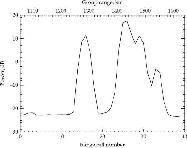
FIGURE 6.2 Average power-delay profile (group range power spectrum) recorded for the Darwin-to-Alice Springs ionospheric link by the Jindalee array at fc = 16.110 MHz on 1 April 1998 between 06:17 and 06:21 UT. © Commonwealth of Australia 2011.
The four peaks in the power-delay profile of Figure 6.2 appear at group ranges of 1290, 1435, 1480, and 1540 km. The locations of these peaks agree well with the group ranges of the modes resolved by the ionogram. Recall that the group range resolution of the power-delay profile is in the order of 20 km, which is not high enough to resolve the two sporadic-E modes in the ionogram at group ranges of 1290 and 1300 km. The mean SNR of the mode(s) represented by each peak of the power-delay profile is estimated as the ratio between the magnitude of the peak and the background noise level estimated from the range cells below 1200 km. Clearly, no modes can be present in these range cells for a 1265-km ground-distance path. In ascending order of group range, the four resolved propagation modes have SNRs of approximately 34.5, 40.5, 34.0, and 20.0 dB.
The capability of the array to isolate the contributions of individual propagation modes into different range bins enables the space-time characteristics of each mode to be studied independently (i.e., separately from the other modes). Specifically, the sequence of “slow-time” samples from one pulse to another in a particular range cell provides information regarding the Doppler characteristics of the propagation mode contained in a particular range cell. Whereas the “array snapshot” samples recorded across different receivers in a particular pulse provides information on the spatial characteristics of the propagation mode in the interrogated range cell. Before proceeding to the fine structure analysis, it is of interest to estimate the nominal gross structure parameters of the ionospheric circuit under study. Apart from estimating the nominal signal-to-noise ratio and time-delay, this also involves estimating the mean direction-of-arrival and Doppler shift of each resolved propagation mode over the period of data collection.
The mean cone angle-of-arrival and Doppler frequency shift of a propagation mode can be estimated by evaluating the conventional angular and Doppler power spectrum using the data in the range cell containing the mode of interest with averaging performed over the data collection interval. Figures 6.3 to 6.6 show the angular and Doppler power spectra resulting for range cells k = 16, 26, 29, 33 which contain the four resolved signal modes. The mean cone angle-of-arrival and Doppler shift of the mode(s) received in each range cell are estimated as the locations of the maxima in the angular and Doppler power spectra, respectively. These estimates are listed in Table 6.1, which summarizes the multipath gross structure parameters of the HF link.

FIGURE 6.3 Conventional Doppler and angle-of-arrival spectrum for the 1Es mode. © Commonwealth of Australia 2011.
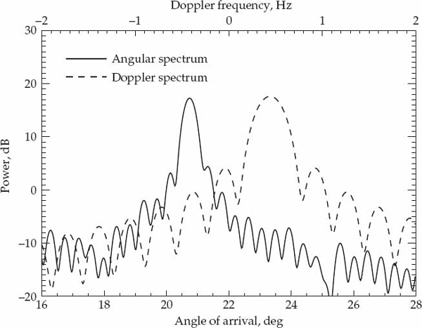
FIGURE 6.4 Conventional Doppler and angle-of-arrival spectrum for the 1F2 mode. © Commonwealth of Australia 2011.
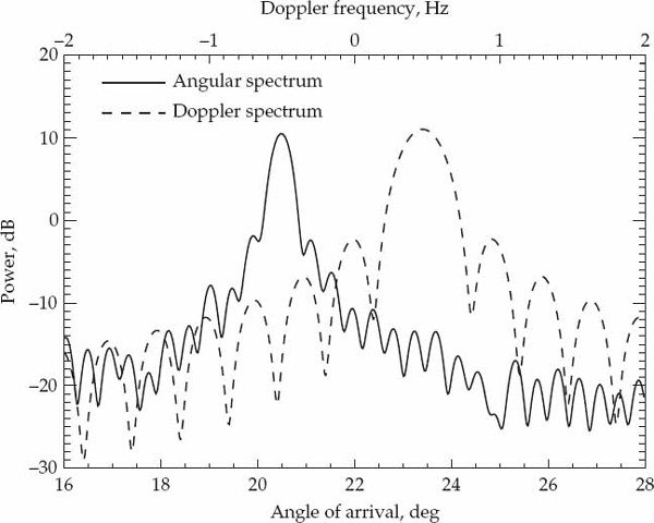
FIGURE 6.5 Conventional Doppler and angle-of-arrival spectrum for the 1F2(o) mode. © Commonwealth of Australia 2011.

FIGURE 6.6 Conventional Doppler and angle-of-arrival spectrum for the 1F2(x) mode. © Commonwealth of Australia 2011.
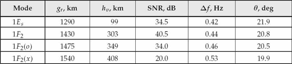
TABLE 6.1 Parameters describing the gross structure of multipath propagation for the Darwin-to-Alice Springs skywave HF link on 1 April 1998 between 06:17 and 06:21 UT.
6.2.3 Fine Structure Observations
Examples of the mode wavefields sampled in space and time over a single CPI may be visualized as intensity-modulated displays in Figures 6.7 to 6.10. These four displays show the real component of the complex valued wavefields sampled over receivers and pulses at range cells k = 16, 26, 29, 33 which coincide with the four peak locations in Figure 6.2. A specularly reflected (plane wave) signal mode would appear as a two-dimensional (space-time) sinusoid in these displays. The spatial frequency of the sinusoid is related to the cone angle-of-arrival, while the temporal frequency is related to the Doppler shift. In the ideal case of specular reflection, the wavefront crests are expected to have equal magnitude and form straight line ridges of constant slope in these displays (i.e., perfectly linear phase-fronts).
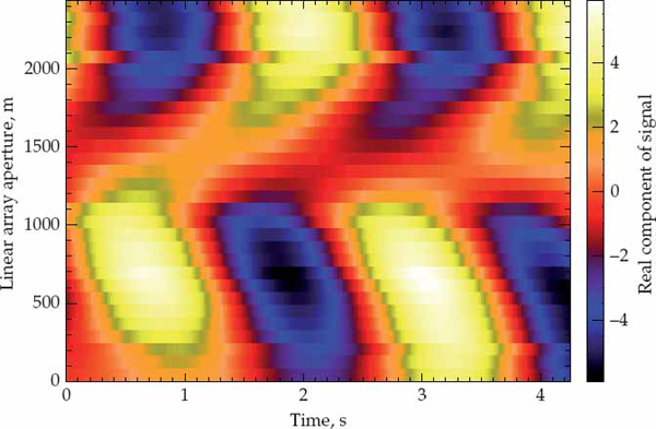

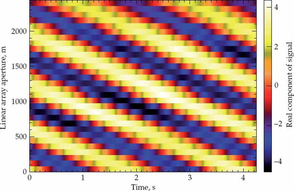

Highly non-planar wavefronts are expected in Figure 6.7 because the wavefield in this range cell results from a superposition of unresolved sporadic-E modes that most likely have different directions-of-arrival. Wavefronts that are more planar in structure are observed for the 1F2 mode in Figure 6.8, which closely resembles a two-dimensional sinusoid. Figures 6.9 and 6.10 display the results for the 1F2(o) and 1F2(x) magneto-ionic components, respectively. The 1F2(o) mode also exhibits relatively planar wavefronts, but it is apparent that the ionospheric reflection process has significantly distorted the 1F2(x) mode. Such distortions are attributable to the presence of ionospheric irregularities because a single magneto-ionic component (i.e., the extraordinary wave of the F2-layer high-angle ray) has been effectively isolated and is not contaminated by other components that could be theoretically expected for a smooth ionospheric layer.
Experimental observations in Rice (1976) and Sweeney (1970) made on a very wide aperture array suggest that a mode wavefront can often be regarded as having a more or less planar large-scale structure with some degree of amplitude and phase corrugations superimposed. At a particular time instant, these corrugations may be viewed as the spatial modulation imparted by the ionosphere on an underlying plane wavefront corresponding to the ideal case of specular reflection. Wavefront tests can be devised to detect the existence of mode fine structure over short time intervals. It is of interest to quantify: (1) the degree of departure of a mode wavefront relative to the plane wave model of best fit at a particular time, and (2) the dynamics of mode wavefront variations as a function of time due to changes in the relative gain and phase of the signal between receiver outputs.
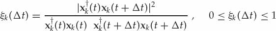
Define xk(t) ∈ CN as the complex N-dimensional array snapshot vector recorded in range cell k and PRI t. A measure of the similarity between the spatial structure of two array snapshots recorded at the same range cell k but in different pulses t and t + Δt is given by the magnitude squared coherence (MSC) function in Eqn. (6.2). The MSC is unity when the snapshots xk(t) and xk(t + Δt) are related by a complex scalar (i.e., have the same spatial structure) and equals zero when the two snapshots become orthogonal. A value between these two extremes indicates the degree of spatial structure variation over Δt PRI, which translates to a time interval of τ = Δt/fp seconds (fp = 60 Hz). Unlike the RMS phase deviation measure used in Rice (1976), the MSC takes both the amplitude and phase of the mode wavefronts into account. Moreover, the condition of unit MSC is invariant to constant array calibration errors, local scattering effects, and the temporal phase rotation introduced by the ionospherically-induced Doppler shift.
(6.2)
Figures 6.11 to 6.14 show the cumulative distributions of MSC values evaluated for different modes and time intervals τ. These distributions were obtained by evaluating MSC for all pairs of array snapshots separated by τ = Δt/fp seconds in 47 dwells of data with each dwell containing P = 256 snapshots. The minimum temporal separation of τ = 1/60 seconds corresponds to curve 1 in all figures and may be regarded as a quasi-instantaneous measure of the MSC. The MSC distributions for longer temporal separations of 1, 2, and 3 seconds are represented by curves 2, 3, and 4, respectively.
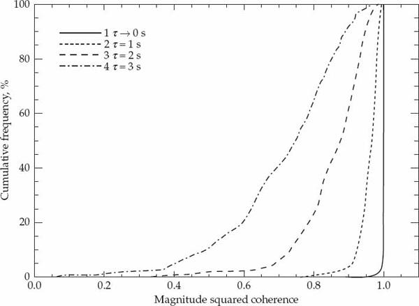
FIGURE 6.11 Cumulative distribution of the MSC for the 1Es mode. © Commonwealth of Australia 2011.

FIGURE 6.12 Cumulative distribution of the MSC for the 1F2 mode. © Commonwealth of Australia 2011.
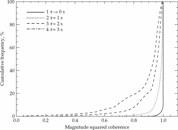
FIGURE 6.13 Cumulative distribution of the MSC for the 1F2(o) mode. © Commonwealth of Australia 2011.
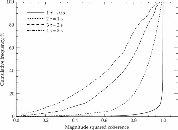
FIGURE 6.14 Cumulative distribution of the MSC for the 1F2(x) mode. © Commonwealth of Australia 2011.
Due to the presence of additive noise, the MSC values will not be exactly equal to unity even when the mode wavefront shape remains perfectly rigid. The effect of additive noise on the MSC distribution is conservatively illustrated by curve 1 in all figures. This assumes that the change in wavefront shape due to physical phenomena is negligible for τ = 1/60 seconds and that departures in the MSC from unity are due to additive noise. If the mode wavefronts retained the same shape over a longer time interval τ, the MSC distributions is expected to resemble curve 1 in all figures because the MSC distribution would be invariant to temporal separation. The results clearly demonstrate that the MSC is highly dependent on temporal separation. This not only confirms the presence of time-varying wavefront distortions due to mode fine structure, but also shows that the mode wavefronts evolve in a correlated manner over time and become progressively different as the temporal separation increases.
The significant reduction in MSC from curve 1 to curve 2 illustrates that changes in spatial structure are appreciable over time intervals as short as 1 second. Curve 1 in Figure 6.13 indicates that 99 percent of the MSC values for the 1F2(o) mode are above 0.95 for τ = 1/60 seconds, while approximately 70 percent of the MSC values drop below 0.95 when the temporal separation is increased to 3 seconds (curve 4 in Figure 6.13). On the basis of this result, it may be claimed with 99 percent confidence that 70 percent of the array snapshots separated by a time interval of τ = 3 seconds do not exhibit the same level of similarity in spatial structure as when the same data snapshots are separated by τ = 1/60 seconds.
The main point is that for very short temporal separations, in the order of an OTH radar PRI, the mode wavefront structure remains essentially fixed, but as the temporal separation increases from a fraction of a second to a few seconds, the dissimilarity between the mode wavefronts gradually increases and becomes quite significant. Although these results quantitatively measure changes in mode wavefront structure as a function of temporal separation, they provide no information regarding the nature of such variations. For instance, it is useful to understand whether such changes are caused by shifts in the nominal cone angle-of-arrival of the underlying plane wavefront, or whether they primarily arise due to fluctuations in the wavefront amplitude and phase corrugations or “crinkles.”
An alternative MSC function that provides this information is formulated in Eqn. (6.3), where s(θ) is the plane wave array steering vector for a cone angle-of-arrival θ. The value of θ that maximizes ρk(t, θ) at time t is denoted by θmax and represents the cone angle-of-arrival of the plane wave that best fits the array snapshot xk(t) in a least squares sense. The maximum value of the MSC itself ρk(t, θmax) is a measure of the goodness of fit between the array snapshot xk(t) and the best fitting plane wave model. In simple terms, ρk(t, θmax) indicates the size of amplitude and phase crinkle on the wavefront. A value of unity is only attained when xk(t) is a plane wave, while lower values indicate the degree of departure of xk(t) from the nearest point on the plane wave array manifold.
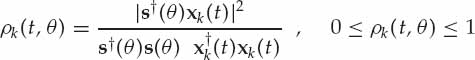
(6.3)
The quantities θmax and ρk(t, θmax) were evaluated for each mode over four successive CPI and plotted in Figures 6.15 to 6.18 as a function of slow time t. Note the inter-dwell gap of approximately 0.5 seconds where no data is recorded. These curves illustrate the temporal behavior of the maximizing argument θmax, which defines the plane wave model of best fit, and the MSC function ρk(t, θmax), which measures the goodness of fit, over time frames commensurate with typical OTH radar CPI. Different vertical axis scales have been used in order to clearly show the variations for different modes.
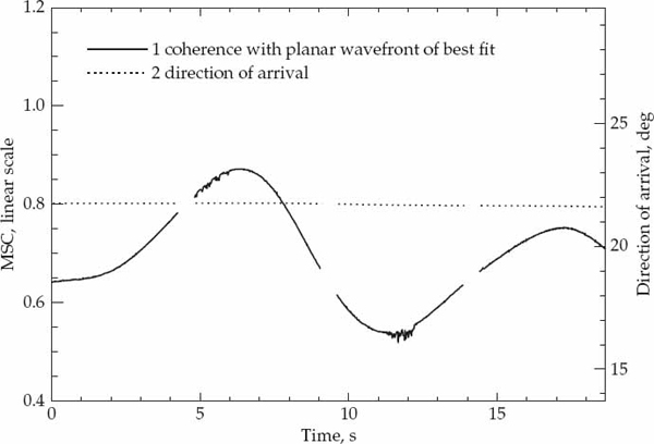
FIGURE 6.15 Analysis of planarity for the array snapshot xk(t) containing the 1Es mode (k = 16). © Commonwealth of Australia 2011.

FIGURE 6.16 Analysis of planarity for the array snapshot xk(t) containing the 1F2 mode (k = 26). © Commonwealth of Australia 2011.
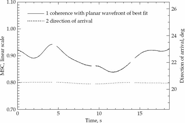
FIGURE 6.17 Analysis of planarity for the array snapshot xk(t) containing the 1F2(o) mode (k = 29). © Commonwealth of Australia 2011.

FIGURE 6.18 Analysis of planarity for the array snapshot xk(t) containing the 1F2(x) mode (k = 33). © Commonwealth of Australia 2011.
With the exception of Figure 6.15, which corresponds to the unresolved sporadic-E modes, the value of ρk(t, θmax) is reasonably close to unity. This supports the view of essentially planar wavefronts. Moreover, the plane waves of best fit to the mode wavefronts remain relatively constant in angle of arrival over a few seconds. This indicates that it is mainly the wavefront distortions or “crinkles” which are changing over time. It is also evident that the degree of fit to the best matched plane wave changes in a rather smooth fashion when sampled at the pulse repetition interval. This indicates that the amplitude and phase modulations imparted on the plane wave of best fit vary in a correlated manner when observed from one PRI to another at a temporal resolution of 1/60 seconds.
The value of ρk(t, θmax) is also subject to additive noise and the presence of array manifold errors. Variations due to additive noise are random from one PRI to another and superimpose on the smooth variations caused by the physical processes evolving in the ionosphere. The effect of noise is most apparent in the Figure 6.18, which corresponds to the mode with lowest signal-to-noise ratio, but is hardly noticeable in the other three figures. Array manifold errors are assumed to be fixed over an observation interval in the order of seconds so their presence would contribute a bias in ρk(t, θmax) but not a variation.
The observed variations in ρk(t, θmax) may therefore be attributed to spatial distortions induced by the ionospheric reflection process on the different propagation modes. An important point is that the precise form of these variations differs substantially from one mode to another. This strongly suggests that spatial distortions induced on a mode reflected by a particular ionospheric region are independent of those induced on another mode reflected by a physically distinct ionospheric region. The practical significance of this observation will be exploited in the final chapter of this text.
The collection of experimental results presented in this section confirm the view that a mode wavefront may be pictured as having an essentially planar spatial structure with some degree of amplitude and phase corrugations superimposed. The analysis has also yielded additional information regarding the time-evolution of individual mode wavefronts over time intervals commensurate with typical OTH radar CPI. While the underlying mean plane wavefront does not vary significantly over a few seconds, the size and shape of the wavefront distortions change gradually in a correlated manner. This leads to the interpretation that the ionospheric reflection process induces changing amplitude and phase distortions about a mean plane wavefront that become progressively de-correlated over time.
6.3 Resolving Fine Structure
To resolve mode fine structure, it is necessary to describe a wave interference model of the HF channel that deterministically represents the signal samples recorded by the antenna array in space and time under standard assumptions and approximations. A mathematical model of the gross structure of the received signal is described first based on the notion of specular reflection from each ionospheric region. This traditional model is then extended by incorporating multiple interfering rays for each propagation mode to parametrically represent fine structure. Robust super-resolution techniques appropriate for estimating the fine structure parameters are then identified and described.
6.3.1 Signal Representation
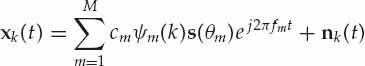
The complex envelope of the baseband space-time digital samples received by the system due to propagation mode m = 1, 2, …, M are denoted by gm( , t, n) in Eqn. (6.4). The fast-time samples acquired during a pulse repetition interval (PRI) are indexed by = 0, 1, …, L − 1, where L = 320 raw A/D samples per sweep in this experiment. The index t = 0, 1, …, P − 1 refers to slow-time samples within each CPI, where P = 256 PRI. The indices and t reference samples collected in time, while the index n = 0, 1, …, N − 1 references spatial samples collected by the N = 32 receivers of the antenna array. The terms Ts and fp respectively denote the fast-time sampling period in seconds and the pulse repetition frequency (PRF) in Hertz. For the collected data, Ts = 52 microseconds and fp = 60 Hz.
(6.4)
Within a given PRI, the frequency of a deramped FMCW signal mode is proportional to its time-delay τm relative to the reference signal when stretch processing is applied. For a single-hop mode propagated over the ground distance of 1265 km, τm typically ranges between 4 and 6 milliseconds. The difference or beat frequency is defined by Δum in Eqn. (6.5), where fb = 20 kHz is the FMCW sweep bandwidth and LTs = 1/fp is the duration of the PRI in seconds. This group-range dependent frequency manifests itself as a regular phase progression ej2πΔumlTs over fast-time samples within each sweep in Eqn. (6.4). The change in group range of a signal mode due to ionospheric motion over typical OTH radar CPI is extremely small compared to the range cell size. Since range cell migration is not an issue in this case, the difference frequency Δum after deramping may be assumed fixed over a CPI of 4.2 seconds.

(6.5)
An ionospheric layer may exhibit a (large-scale) uniform component of motion that imposes a regular Doppler shift on the reflected signal mode. The Doppler shift imposed by the ionosphere on mode m is defined by Δfm in Eqn. (6.6), where fc = 16.110 MHz is the carrier frequency, c = 3.0 × 10⁸ m/s is the speed of light in free space, and vm is the relative velocity (group range rate) of the mode. A positive Doppler shift indicates that the effective reflection point is moving “downwards,” shortening the phase path of the mode with respect to time, while the reverse applies when the Doppler shift is negative.
(6.6)
The relative velocity vm of the reflection point is typically less than 10 m/s for quiet mid-latitude paths. This corresponds to a Doppler shift of 1 Hz for a single reflection at a carrier frequency of 15 MHz. Over a 4.2-second CPI, the effective displacement of the reflection point at this velocity is 42 m, which results in a differential time-delay of δτm = 1.4 ns between endpoints of the CPI. As the time-bandwidth product condition in Eqn. (6.7) is satisfied, the Doppler effect manifests itself as a regular phase progression or frequency shift ej2πΔfmt/fp in Eqn. (6.4). For vm = 10 m/s, it would take over 15 minutes before the change in virtual reflection height causes the mode to migrate by one range cell.
(6.7)
The initial phase of mode m at the start of the CPI relative to that of the transmitted waveform is given by γ(τm) in Eqn. (6.8) for a linear FMCW signal. This term depends on the mode time-delay tm at the beginning of the CPI in the reference (first) receiver and determines the starting phase relationship among the modes. The scalar Am is an attenuation factor that accounts for all losses in the mode amplitude between the transmitter and receiver.
(6.8)
With reference to Figure 6.19, the ULA is aligned along the x-axis with the reference antenna at the origin. The N subarray centers of the Jindalee array are spaced Δd = 84 m apart. Consider a plane wave signal mode incident upon the ULA at azimuth αm relative to boresight and elevation βm after specular reflection from the ionosphere. In this experiment, the great circle bearing of the test transmitter is 22 degrees. The elevation β depends on the virtual reflection height and typically varies between 5 and 35 degrees for single-hop ionospheric modes over a 1265-km mid-latitude path. By defining 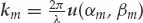 as the signal wavevector, where u(αm, βm) = [cos βm sin αm, cos βm cos αm, sin βm]T is a unit vector in the wave propagation direction and λ = c/fc is the carrier wavelength, the relative phase of the carrier at receiver n in the array with respect to the reference receiver at the origin is calculated as the inner product km·rn in Eqn. (6.9), where rn = [nΔd, 0, 0]T is the position vector of receiver n.
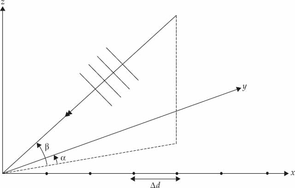
FIGURE 6.19 Three-dimensional coordinate system showing a plane wave incident from azimuth α and elevation β on a ULA aligned along the x-axis.
(6.9)
The differential time-delay between opposite ends of the array is given by Eqn. (6.10) which is in the order of 2–3 microseconds for αm = 22 degrees, βm = 5–35 degrees, and (N − 1) Δd = 2.8 km. Such delays correspond to a time-bandwidth product much less than unity for a radar signal bandwidth fb = 20 kHz, so the phase relationship over different receivers may be written as ejkm·rn in accordance with the narrowband assumption. The spatial phase difference may be interpreted in terms of the cone angle-of-arrival θm subtended by the mode wavevector and the x-axis. When the cone angle is interpreted as a bearing for a source off boresight, the apparent azimuth of the source approaches boresight as the mode elevation angle increases. This “coning effect” often allows different propagation modes from a single source to be resolved in cone angle by a ULA.
(6.10)
Range processing is performed by taking the weighted fast Fourier transform (FFT) of the fast-time samples in each PRI. The range bins retained for further processing are indexed by k = 0, 1, …, K − 1, where K = 42 corresponds to a range depth of 630 km in this case. The range processing FFT of Eqn. (6.4) over all pulses and receivers yields the output sm(k, t, n) in Eqn. (6.11), where cm = Amejγ(τm) is the mode complex amplitude and  is the range spectrum point spread function defined by the Fourier transform of the Hanning window used for range processing. This function is normalized such that f(0) = 1.
(6.11)
The received data x(k, t, n) is the sum of M modes sm(k, t, n) for m = 1, …, M and uncorrelated noise. The array snapshots xk(t) = [x(k, t, 0), …, x(k, t, N − 1)]T received by the antenna array at range bin k and PRI t may be written as in Eqn. (6.12), where fm = Δfm/fp is the mode Doppler shift normalized by the PRF and 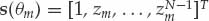 is the plane wave array steering vector defined in terms of
  .
.
(6.12)
The additive noise is often modeled as temporally and spatially white with second-order statistics given by Eqn. (6.13). Here,  denotes the nth element of nk(t), E{·} is the statistical expectation operator, and δ(·) is the Kronecker delta function. Residual noise correlation in range due to the FFT window function has been ignored here.
(6.13)
Let km be the range cell most closely matched to mode m. Provided the different modes are well resolved in group range, the M mode waveforms can be effectively separated into different range cells  with negligible contamination from neighboring modes. In other words, contributions due to the mismatched modes may be neglected at cell km when the spectral leakage in range falls below the noise level. In this case, we can make the approximation ψm(k) = δ(k − km), such that xkm (t) is effectively given by Eqn. (6.14).
(6.14)
It has been conjectured that individual propagation modes may be composed of a small number of (presumably specular) components or “submodes” unresolved in time-delay but with different Doppler shifts and closely spaced directions-of-arrival. For a smooth layer, the unresolved submodes may correspond to the four theoretically expected rays (high/low, ordinary/extraordinary) or a subset of them, whereas for a single resolved magneto-ionic component, these submodes can only originate from electron density irregularities in the ionosphere. The wave interference model of fine structure represents the mode in range km as the sum of Rm submodes or rays in Eqn. (6.15).

(6.15)
The distinction between the gross and fine structure of an individual propagation mode resolved in range is that the latter contains more than one term (i.e., Rm > 1) in the wave interference model. The wave interference model in Eqn. (6.15) is deterministic, whereas the Doppler shift, direction of arrival, and other parameters of real ionospheric modes are expected to change over time. The scope of such a model is therefore to represent mode fine structure over a limited time commensurate with typical OTH radar CPI (i.e., in the order of a few seconds).
6.3.2 Parameter Estimation
Define the NP-dimensional stacked vector  as the space-time data sampled over all receivers and pulses in range cell km during the CPI. By restricting attention to a single range cell for the time being, the data vector corresponding to the analyzed mode may be simply referred to as z. The signal component in z is assumed to result from the interference of R rays that model the fine structure of the signal mode. In accordance with Eqn. (6.15), the data vector may be written in the form of Eqn. (6.16), where A(φ) is a NP × R mixing matrix to be defined shortly, the vector c = [c1, …, cR] contains the ray complex amplitudes (i.e., magnitudes and initial phases) as its elements, and n is the stacked vector of additive noise defined similarly to z.
(6.16)
The R columns of the mixing matrix A(φ) are composed of ray space-time steering vectors a(θr, fr) ∈ CNP for r = 1, …, R. The matrix A(φ) is therefore defined by the functional form of the space-time manifold a(θ, f) and the fine structure parameter vector φ = [θ1, θ2, …, θR, f1, f2, …, fR]T, which contains the cone angles-of-arrival and normalized Doppler frequency shifts of the R rays.
(6.17)
The NP-dimensional space-time manifold a(θ, f) may be expressed as the Kronecker product ( ) between the N-dimensional spatial steering vector s(θ) defined previously and the P-dimensional temporal steering vector v(f) = [1, ej2πf, …, ej2π(P−1)f]. The manifold a(θ, f) has a Vandermonde structure, which implies that any given steering vector cannot be expressed as a linear combination of other steering vectors on the manifold.
(6.18)
Ideally, the maximum likelihood estimate of the ray parameters is given by Eqn. (6.19). However, it is quite common for the parameter vector and ray complex amplitudes to be estimated separately rather than jointly. Provided the parameter estimation technique is chosen and implemented judiciously, as described in the next section, such approaches can yield comparable estimates to the ML technique in a more computationally efficient manner.
(6.19)
For the assumed number of rays R, the first task is to estimate the parameter vector φ from the data z. Based on this estimate, denoted by  , it is possible to reconstruct an approximation of the mixing matrix as Α(). The ray complex amplitudes may then be estimated as the vector
  that provides the best least squares fit to the measured data z in accordance with Eqn. (6.20), where ||·||2 represents the L2-norm (also known as the Frobenius norm ||· ||F) and
  is the Moore-Penrose pseudo-inverse of Α(). Stated another way, the ray complex amplitudes are estimated so as to minimize the power of the residual error between the model
  and measured data z.
(6.20)
Once the model order is selected and the ray parameters are estimated, the second task is to evaluate the accuracy with which the wave interference model represents the fine structure of real ionospheric modes sampled in space and time. A quantitative measure of the match between the simulated space-time data and the experimentally received signal samples is required to evaluate the performance of the wave-interference model as well as to establish criteria for accepting or rejecting its validity. A performance metric that is intuitively appealing and relatively simple to calculate is the ratio of the energy in the residual error  to that of the experimental data ||z||2. The model-fitting accuracy (MFA) metric defined in Eqn. (6.21) expresses the fit of the model to the data based on this criterion as a percentage.

(6.21)
The model  is considered to be a satisfactory representation of the received data z when the MFA is sufficiently close to its upper limit of 100 percent. The meaning of “sufficiently close” should be defined with respect to the signal-to-noise ratio as the MFA will be less than 100 percent even if the model exactly replicates the signal component of the received data due to the presence of additive noise. From Eqn. (6.21), it is relatively simple to show that the expected value of the MFA for perfect signal modeling and uncorrelated additive noise is given by SNR/(SNR+1), where SNR is the signal-to-noise ratio. For the high SNR modes in the analyzed data, the MFA will most likely be limited by modeling errors rather than additive noise.
As far as resolving the fine structure of a propagation mode is concerned, the problem of estimating the ray parameter vector and complex amplitudes is a challenging one in practice. This is because the constituent rays will typically have closely spaced Doppler shifts and cone angles-of-arrival. Two rays with the same Doppler shift but different angles of arrival will produce a non-planar wavefront at the receivers that does not change over time. On the other hand, two rays with the same angle of arrival but different Doppler shifts will produce a plane wave that exhibits fading in time. In general, different rays have slightly different angles of arrival and Doppler shifts, which results in time-varying and non-planar wavefronts. This qualitative interpretation of a mode wavefront is consistent with the experimental observations made in Section 6.2.3.
Classical spectrum estimation techniques based on the FFT algorithm (periodogram) are computationally efficient.1 A disadvantage of such techniques is that the mainlobe width prevents the resolution of two or more frequency components that are mutually spaced closer than the reciprocal of the data length. Another disadvantage is that strong signals can leak through the sidelobes and potentially mask a relatively weaker signal in the main lobe. The single dominant peaks in Figures 6.3 to 6.6 clearly show the inability of classical angle and Doppler spectrum estimation to resolve multiple rays within a mode due to the aforementioned drawbacks. Such techniques are therefore unsuitable for resolving the fine structure of individual propagation modes in the HF environment.
Other methods based on linear prediction Marple (1987) or the minimum variance distortionless response (MVDR) estimator Capon (1969) may be considered, but the best frequency resolution and estimation performance has been attributed to techniques based on the eigenstructure of the sample covariance matrix. The basis for improved performance, especially at lower signal-to-noise ratios, stems from the division of the information contained in the sample covariance matrix into signal and noise vector sub-spaces. The tremendous interest in subspace methods mainly originates from the initial development of the MUltiple SIgnal Classification (MUSIC) algorithm, Schmidt (1981). Since the introduction of MUSIC, a large variety of different super-resolution algorithms have emerged. An excellent summary of these algorithms and their relative merits can be found in Krim and Viberg (1996). A description of MUSIC is not repeated here for brevity, but the reader is referred to Marple (1987) for a detailed exposition of the essential concepts.
The maximum likelihood (ML) estimator mentioned earlier is a parametric method that can outperform MUSIC, particularly when two or more rays are coherent or highly correlated over the observation interval, see Krim and Viberg (1996). However, the ML estimator is computationally intensive relative to MUSIC, and perhaps more importantly, its convergence to the global optimum of the objective function in Eqn. (6.19) is not always guaranteed. In addition, sub-aperture smoothing techniques described in Pillai (1989) can be applied to improve the performance of MUSIC in the presence of correlated arrivals. MUSIC is identified as a suitable compromise between resolution power, computational complexity, and the capability to perform joint space-time frequency estimation in this application.
While MUSIC inherently estimates the parameters of different rays separately, it is possible to estimate the spatial and temporal frequencies of a particular ray jointly. Application of space-time MUSIC allows the different rays to be discriminated simultaneously in two dimensions rather than only in one. For example, two rays with almost identical Doppler shifts may not be resolved in temporal frequency, but if their cone angles-of-arrival are sufficiently different, it is theoretically possible to resolve the two rays as different peaks in the space-time domain. Another advantage of joint space-time processing is that pairing of the ray angle-of-arrival and Doppler frequency estimates occurs automatically since each ray is resolved on a two-dimensional (space-time) search grid. Disadvantages include the extra computational effort due to the use of covariance matrices with higher dimensionality, the larger amount of data required to estimate such matrices accurately, and the two-dimensional search instead of two one-dimensional searches.
6.3.3 Space-Time MUSIC
To describe the space-time MUSIC technique, let xk(s, t) be an Ns-dimensional array snapshot vector recorded by Ns receivers of the antenna array starting at receiver number s, where s ∈ [0, N − Ns] and Ns < N. Unlike the full-aperture array snapshot xk(t) ∈ CN, which contains all receiver outputs, xk(s, t) ∈ CNs represents a sub-aperture of the ULA that contains Ns consecutive receiver outputs with the first element corresponding to receiver index s. The space-time data vector zk(s, t, Δt) ∈ CNsNt in Eqn. (6.22) is formed by stacking the Ns-dimensional array snapshots xk (s, t) recorded over Nt slow-time samples spaced Δt PRI apart such that t ∈ [0, P − NtΔt] and NtΔt < P. It is assumed that the values of Ns and Nt are chosen such that NsNt > R, and that the R rays have distinct parameter tuples {θ, f}.
(6.22)
The space-time data vector zk(s, t, Δt) can be written as Eqn. (6.23), where A(φ) is the reduced dimension NsNt × R mixing matrix. To avoid complicated notation, the sub-aperture ray mixing matrix in Eqn. (6.23) is not distinguished from the full-aperture version defined previously in Eqn. (6.17).
(6.23)
The M-dimensional signal vector sk(t) in Eqn. (6.24) contains the complex waveforms sm(k, t, s) recorded for each ray at the starting receiver (s). The space-time vector of uncorrelated white noise nk(s, t, Δt) is constructed in analogous fashion to Eqn. (6.22) and represents the additive noise component of the space-time vector zk(s, t, Δt).
(6.24)
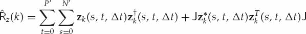
Traditionally, the space-time sample covariance matrix used to compute the MUSIC spectrum is estimated using the full array aperture. When two or more rays are coherent (i.e., have the same Doppler shift), the standard MUSIC spectrum fails to provide consistent estimates of all the ray angles-of-arrival and Doppler shifts. This occurs due to a rank deficiency in the dimension of the signal subspace, as discussed in Pillai (1989). To rectify this situation, the idea of spatial smoothing described in Shan, Wax, and Kailath (1985) and Pillai and Kwon (1989) may be employed to “de-correlate” the rays while preserving the angular and Doppler information. Specifically, the forward-backward spatial smoothing technique is used to form the sample space-time matrix  in Eqn. (6.25), where P′ = P − NtΔt, N′ = N − Ns and J is the square NsNt × NsNt-dimensional exchange matrix with ones on the anti-diagonal and zeros elsewhere.
(6.25)
The statistically expected space-time covariance matrix Rz(k) takes the form of Eqn. (6.26), where Sk ∈ CR×R is referred to as the spatially smoothed source covariance matrix. Although the true source covariance matrix defined as  is not full rank when two or more signals are coherent, it can be shown that the rank of the spatially smoothed source covariance matrix increases by one with probability one for each spatial average (Pillai 1989). This property allows MUSIC to yield consistent estimates of the ray parameters when two or more rays are coherent or highly correlated. The cost of sub-aperture smoothing is a reduction in resolution and the maximum number of rays that can be resolved.
(6.26)
Assuming Sk has full rank R, the eigen-decomposition of the positive definite Hermitian matrix Rz(k) may be expressed as in Eqn. (6.27), where the R columns of Qs contain the eigenvectors spanning the signal subspace. A critical point is that the span of the signal eigenvectors is identical to the range space of A(φ). On the other hand, the NsNt − R columns of Qn are noise eigenvectors spanning the orthogonal subspace to Qs and hence A(φ). The diagonal matrix Λ = diag[λ1, …, λR] contains the largest eigenvalues associated with the R principal eigenvectors, while the smaller (noise) eigenvalues are all equal to  .
.
(6.27)
As the eigenvectors in the signal subspace are orthogonal to those in the noise subspace, the ray vectors a(θr, fr) are also mutually orthogonal to the noise subspace eigenvectors. In other words,  when the parameters θ = θr and f = fr for r = 1, 2, …, R. Moreover, the parameter tuples {θr, fr} corresponding to the R rays are the only possible cone angle and Doppler shift combinations that can satisfy this orthogonality condition because any collection of distinct space-time signal vectors a(θ, f) forms a linearly independent set. The spatially smoothed MUSIC spectrum pmu(θ, f) in Eqn. (6.28) may therefore be computed by projecting a spectrum of signal vectors a(θ, f) against the estimated noise subspace
  calculated from the sample space-time covariance matrix
  in Eqn. (6.25).
(6.28)
The MUSIC spectrum exhibits sharp peaks in the vicinity of the true ray angles-of-arrival and Doppler shifts. The coordinates of these peaks yields the parameter vector estimate . The magnitude of the peaks in the MUSIC spectrum should not be interpreted as the amplitude of the rays. The ray complex amplitudes are estimated separately using the least squares procedure in Eqn. (6.20).
6.4 Experimental Results
The described space-time MUSIC technique requires the model order or number of rays to be specified. A method based on information theory that uses the eigenvalues of the sample covariance matrix to estimate the number of rays was developed by Wax and Kailath (1985). Although such a method is applicable here, it should be kept in mind that the objective is to determine how well a small number of rays can represent mode fine structure. A model involving a high number of rays can always be constructed in principle to represent mode fine structure very accurately. However, such a model is of limited utility for a number of reasons. First, the physical significance of the model is more readily interpreted when the data characteristics can be represented by a small number of rays; and second, models of very high order are less mathematically tractable and require many parameters to specify.
At the other extreme, a one-ray model is too simplistic and does not satisfactorily represent the observed HF channel characteristics. Models of intermediate complexity are of most practical benefit because they are challenging enough to allow the performance of different algorithms to be meaningfully compared and ranked, but not so challenging as to defeat them all. The question arises as to what constitutes the meaning of the term “relatively few rays” or “a small number of rays.” Two- and three-ray wavefields were synthesized by Gething (1991) in order to compare the performance of different wavefront analysis techniques. The same model orders were adopted by Rice (1982) to analytically derive probability density functions for a defined measure of wavefront planarity. In this section, the ability of the model to characterize mode fine structure using up to four rays is analyzed. The major justification for going to four rays is that it coincides with the number of rays that are theoretically expected after reflection from a single smooth ionospheric layer.
6.4.1 Preliminary Data Analysis
In addition to the model order R, the sub-aperture dimensions also need to be specified in terms of the number of receivers Ns, the number of temporal taps Nt, and the spacing between adjacent taps Δt. While higher values of Ns, Nt, and Δt improve resolution, the larger sample covariance matrix dimension that results leads to an increase in the variance of the MUSIC spectrum estimates when using a finite set of space-time data. Use of data from multiple CPI to stabilize these estimates is not recommended because there is a greater chance of the ray parameters changing as the observation interval increases.
There are no definitive guidelines for selecting the “optimum” array sub-aperture dimensions when the signal environment is unknown a priori. In the following analysis, the space-time MUSIC spectra were estimated using Ns = 16 receivers, Nt = 16 temporal taps, and Δt = 12 PRI (i.e., a 0.2-second tap spacing). Based on the premise of limiting the duration of the analysis to a single CPI of data at a time, these values were empirically chosen to trade off the resolution and variance of the parameter estimation technique so as to yield satisfactory performance.
To compare the experimental application of one- and two-dimensional MUSIC for the problem of resolving mode fine structure, the smoothed spatial-only MUSIC spectrum is obtained by setting Nt = 1 and Ns = 16, while the temporal-only version is computed by setting Ns = 1 and Nt = 16 with Δt = 12. The first example considers the 1Es mode received in a particular CPI. The real component of the space-time wavefield received for this mode was previously illustrated in Figure 6.7.
Curves 2 and 3 in Figure 6.20 illustrate the spatial-only MUSIC spectra assuming a model order of four and five rays respectively. Note that the four peaks resolved for M = 4 become broader when M = 5 is assumed but a fifth peak does not appear. This suggests the presence of four dominant rays that can be resolved in angle-of-arrival. Curve 1 in Figure 6.20 shows the standard MUSIC spectrum without spatial smoothing for the same data (i.e., Ns = N = 30). Curve 4 in Figure 6.20 relates to the right vertical axis and represents the MVDR spectrum using the same spatially smoothed sample spatial covariance matrix as that used to compute the MUSIC spectra in curves 2 and 3.
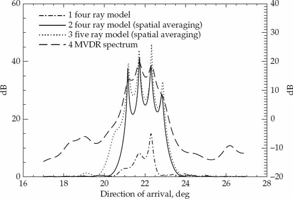
FIGURE 6.20 Spatial MUSIC spectra for the 1Es mode (k = 16). The angles of arrival corresponding to the four peaks in Curve 2 are 21.2, 21.7, 22.3, and 22.8 degrees. The scale on the right vertical axis corresponds to the MVDR spectrum (curve 4) only. © Commonwealth of Australia 2011.
A comparison of curves 2 and 4 in Figure 6.20 illustrates that the spatial-only MUSIC algorithm can resolve four closely spaced rays while the MVDR only resolves three. The presence of the fourth ray is indicated by a slight bulge in the MVDR spectrum at the angle of the unresolved ray. This illustrates the superior resolution of the subspace method, as expected. A comparison of curves 1 and 2 in Figure 6.20 illustrates the benefit of spatial smoothing that allows four rays to be resolved. The poor performance of the standard (unsmoothed) MUSIC algorithm in this example suggests the presence of highly correlated arrivals during the observation interval. This suggests the presence of rays with very similar Doppler shifts.
Using the same data, curves 1, 2, and 3 in Figure 6.21 illustrate the temporal-only MUSIC spectra for an assumed model order of one, two, and three rays, respectively. All three MUSIC spectra relate to the left vertical axis and were evaluated for the sample temporal covariance matrix using Nt = 16 and Δt = 12. Curve 4 relates to the right vertical axis and shows the MVDR spectrum computed using the same sample covariance matrix as MUSIC. Despite four rays being resolved in the angular MUSIC spectrum, only two rays can be resolved in Doppler frequency by MUSIC. The inability of temporal-only MUSIC to resolve more than two rays is consistent with the previous suggestion that some of the rays have very similar Doppler shifts.
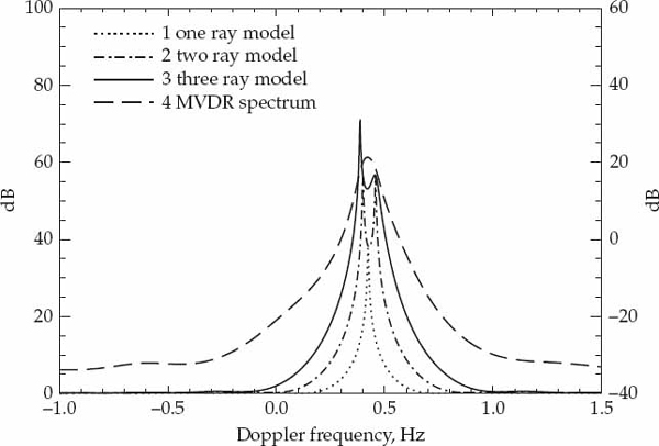
FIGURE 6.21 Temporal MUSIC spectra for the 1Es mode (k = 16). The Doppler frequencies corresponding to the two peaks in Curve 2 are 0.40 and 0.46 Hz. The scale on the right vertical axis corresponds to the MVDR spectrum (curve 4) only. © Commonwealth of Australia 2011.
Although the MVDR spectrum is often referred to as a high-resolution estimator, it cannot resolve the two rays resolved by MUSIC in Figure 6.21. This is a further illustration of the superior performance of the MUSIC super-resolution algorithm. Nevertheless, the MVDR spectrum is important because it indicates that most of the received power is distributed in an interval of Doppler frequencies between 0.4 and 0.6 Hz. If four dominant rays are present, then the Doppler frequencies of these rays are expected to be in this interval.
The discrepancy between the number of rays resolved in angle-of-arrival and Doppler frequency creates a problem when it comes to analyzing the wavefield since it is not possible to unambiguously assign a spatial and temporal frequency to each ray. This real-data example serves to illustrate the principal motivation for using space-time MUSIC rather than estimating the parameters via two one-dimensional MUSIC spectra. The space-time MUSIC spectrum derived from the same data using Ns = 16, Nt = 16, Δt = 12 and assuming four rays is shown as a three-dimensional surface plot in Figure 6.22.

FIGURE 6.22 Space-time MUSIC spectrum for the 1Es mode assuming four rays. © Commonwealth of Australia 2011.
The parameters of the four rays resolved for the 1Es mode by the space-time MUSIC spectrum in Figure 6.22 are listed in Table 6.2. This includes the amplitude and initial phase of each ray that were estimated using the least squares procedure in Eqn. (6.20). Note that the location of each peak resolved by the temporal-only and spatial-only MUSIC spectra is consistent with the coordinates of one of the four peaks resolved in the space-time MUSIC spectrum. The space-time MUSIC spectrum also confirms that three of the four rays have almost identical Doppler shifts. These three rays were not resolved by temporal-only MUSIC, but were resolved by the smoothed spatial-only and space-time MUSIC techniques due to their different angles of arrival.
Examples of the space-time MUSIC spectra resulting for the 1F2, 1F2(o), and 1F2(x) modes are shown in Figures 6.23 to 6.25. For each mode, the model order was chosen to represent the number of rays that were frequently required to yield a fitting accuracy greater than 90 percent over the entire data set containing 47 CPI. The ray parameters estimated from these space-time MUSIC spectra are also listed in Table 6.2.

FIGURE 6.23 Space-time MUSIC spectrum for the 1F2 mode assuming three rays. © Commonwealth of Australia 2011.
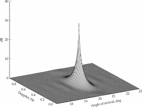
FIGURE 6.24 Space-time MUSIC spectrum for the 1F2(o) mode assuming one ray. © Commonwealth of Australia 2011.

FIGURE 6.25 Space-time MUSIC spectrum for the 1F2(x) mode assuming two rays. © Commonwealth of Australia 2011.

TABLE 6.2 Ray parameters estimated from space-time MUSIC spectra computed for the 1Es, 1F2, 1F2(o), and 1F2(x) modes using a single CPI of data. © Commonwealth of Australia 2011.
6.4.2 Model-Fitting Accuracy
Figures 6.26 to 6.29 summarize the results of this experimental analysis by showing the fitting accuracy achieved for each mode as a function of the number of rays and the particular CPI of data analyzed. Note that certain CPI in Figures 6.26 to 6.29 do not contain a measurement for all model orders because the number of peaks resolved by the space-time MUSIC spectrum does not always coincide with the assumed number of rays. This situation may arise when the model order is overestimated or if the rays are present but cannot be resolved. The fitting accuracy is not displayed when the number of peaks does not agree with the assumed model order.
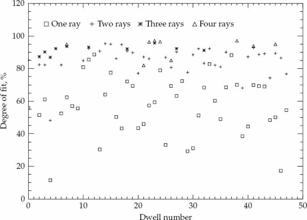
FIGURE 6.26 Fitting accuracy for the 1Es mode. © Commonwealth of Australia 2011.
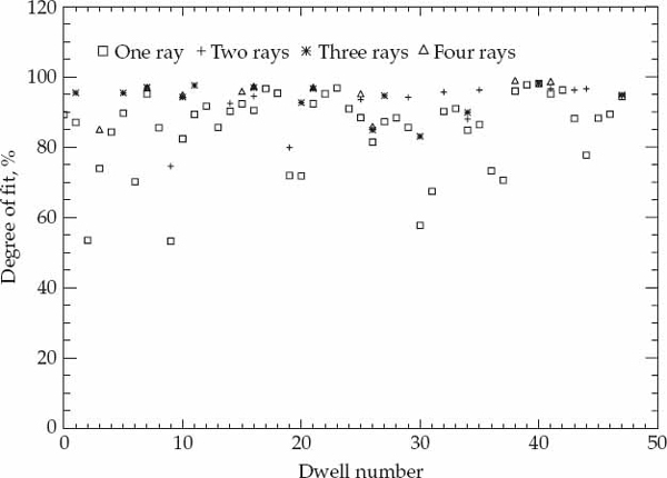
FIGURE 6.27 Fitting accuracy for the 1F2 mode. © Commonwealth of Australia 2011.
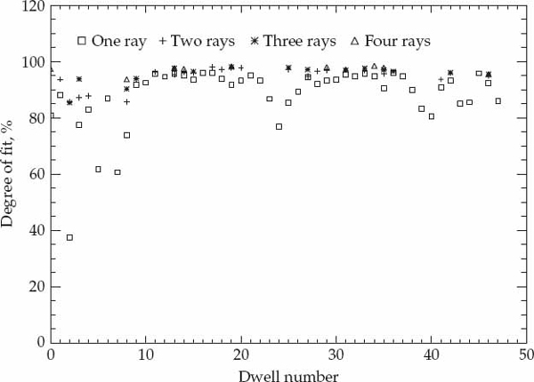
FIGURE 6.28 Fitting accuracy for the 1F2(o) mode. © Commonwealth of Australia 2011.
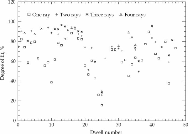
FIGURE 6.29 Fitting accuracy for the 1F2(x) mode. © Commonwealth of Australia 2011.
It is important to note that the failure of MUSIC to resolve the expected number of peaks does not imply that a wave interference model having less than the assumed number of rays cannot adequately represent the data. For example, the assumption of two and three rays for the 1F2 mode in dwell 22 gives rise to one and two peaks, respectively, so the symbols corresponding to these model orders do not appear for dwell number 22 in Figure 6.27. However, the fitting accuracy achieved by the two resolved rays when three rays were assumed was 93 percent.
Figure 6.30 shows the real component of the model wavefield using the ray parameters estimated for the 1Es mode in Table 6.2. Upon visual inspection, this simulated wavefield is very similar to the experimentally recorded one shown in Figure 6.7. A quantitative comparison between the real and simulated complex wavefields is made in terms of the MFA metric defined in Section 6.3.2. In this example, the estimated four ray interference model yields a fitting accuracy of 96 percent. From a physical perspective, the two rays with cone angles less than the great circle azimuth of the test transmitter (22 degrees) and the two rays with cone angles larger than 22 degrees are possibly reflected from different clouds of sporadic-E ionization.

At least two rays are expected for the 1F2 mode as this mode is theoretically composed of both the ordinary and extraordinary rays in the low-angle path. Inspection of Figure 6.27 reveals that three-rays are resolved more often than two-rays for this mode. Furthermore, a three-ray model at times yields a significantly better fitting accuracy compared with the two-ray model. For example, the three-ray model depicted by the space-time MUSIC spectrum in Figure 6.23 led to a fitting accuracy of 95 percent as compared to 87 percent for a two-ray model. When a third ray is resolved, it is thought to account for ionospheric irregularities in F-region.
In the absence of ionospheric irregularities, a one-ray model is expected to provide an accurate description of the wavefield produced by a single magneto-ionic component. As shown in Figure 6.28, this was found to be the case for the 1F2(o) mode in most of the CPI analyzed. A high fitting accuracy using a single ray also indicates that the ULA has a steering vector that is accurately matched at the carrier frequency to the one expected in the absence of calibration errors. In the example of Figure 6.24, a single ray provided a fitting accuracy of 95 percent for the 1F2(o) mode.
Figure 6.29 shows that a single ray is not able to represent the 1F2(x) mode wavefields as well as those of the 1F2(o) mode. The extraordinary magneto-ionic component is reflected from a different region in the F2-layer, which on this occasion appears to be relatively more disturbed than the region that reflected the ordinary magneto-ionic component. For the 1F2(x) mode, it was found that two or more rays were often needed to yield fitting a accuracy above 90 percent. Two rays were resolved more often than three or four rays for this particular mode and the fitting accuracy achieved using a two-ray model was usually considerably higher than that for one ray. For example, the two-ray model corresponding to the spectrum in Figure 6.25 resulted in a fitting accuracy of 94 percent, whereas a one-ray model only fitted the data to an accuracy of 82 percent.
To illustrate the time-variation of ray parameters from one dwell to another, consider a two-ray representation of the 1Es mode. Figure 6.31 shows the variation in the estimated cone angles-of-arrival and Doppler shifts of the two rays for dwells in which the fitting accuracy was greater than 85 percent. The time-variation of the ray angles-of-arrival is in the order of 0.5 degrees over the 47 CPI analyzed, while the Doppler shifts vary by approximately 0.1 Hz. The observed variation in ray parameters from dwell to dwell is expected due to the movement of the effective reflection points in the ionosphere over time intervals in the order of a few minutes.

FIGURE 6.31 Dwell-to-dwell variation of the estimated angles of arrival and Doppler shifts of a two-ray model for the 1Es mode. © Commonwealth of Australia 2011.
6.4.3 Summary and Discussion
The fine structure of HF signal modes reflected from different layers in the ionosphere is considered by some investigators to result from a superposition of relatively few specularly reflected rays having similar Doppler shifts (to account for the observed temporal fading) and closely spaced directions-of-arrival (to account for the observed wavefront distortions). However, the resolution of a complex-valued space-time mode wavefield into a number of component rays with a very wide aperture antenna array has received insufficient attention in practice. Such analysis is considered valuable as it provides quantitative information regarding the capability of such a model to represent the mode wavefields received by a very wide aperture array over typical OTH radar CPI.
After a preliminary analysis of mode fine structure that demonstrated the existence and characteristics of mode wavefront distortions within typical OTH radar CPI, the MUSIC space-time parameter estimation technique was used to resolve the fine structure of individual ionospheric modes recorded by the Jindalee receiving array on a controlled mid-latitude propagation path. A performance measure was developed to assess the accuracy with which the model was able to fit the experimentally recorded wavefields, and the physical significance of the resolved rays was also tentatively interpreted on the basis of an oblique incidence ionogram recorded for the path.
The experimental results indicate that over time intervals in the order of a few seconds, the ionospheric modes received by the Jindalee antenna array could be represented to fitting accuracies above 90 percent using four rays or less over a large percentage of the analyzed data set. However, time-variations of the ray parameters were observed from one CPI to another as a result of motions in the ionosphere. These variations imply that as the CPI increases, the number of rays required to maintain a given modeling accuracy will also increase. Consequently, the wave interference model may be regarded as appropriate for representing a quiet mid-latitude HF channel in a deterministic manner over an interval of a few seconds, but is not suitable for representing the characteristics of a longer data set received over an interval of a few minutes.
____________________
1 The term spectrum estimation is used rather than frequency estimation because the periodogram also estimates the power of the sinusoids in the data.
..................Content has been hidden....................
You can't read the all page of ebook, please click here login for view all page.