
CHAPTER 9
Interference Cancelation Analysis
The space-time characteristics of HF signals reflected by the ionosphere have been analyzed and modeled from a signal-processing perspective in Chapters 6–8. The physical phenomena that contribute to the observed signal characteristics are clearly of scientific interest, but the more pragmatic question arises as to the practical impact of space-time signal distortions in operational OTH radar systems. The first objective of this chapter is to present the results of a case study that demonstrates the influence of such distortions in a key OTH radar signal-processing application. Specifically, this case study experimentally quantifies the performance of different adaptive beamforming schemes applied to the problem of HF interference cancelation in OTH radar.
The HF channel model described in Chapter 8 was empirically shown to accurately represent the statistical characteristics of signal modes reflected by the ionosphere. While this condition is considered necessary for experimental validation, realizations of the model are also required to accurately portray the performance of signal-processing techniques applied to real data. A simulator with this capability not only helps to guide algorithm design, but also serves to evaluate the relative merits and shortcomings of different signal-processing techniques in a convenient manner. It is therefore of interest to determine the fidelity with which the previously described multi-variate HF channel model and parameter estimation technique can predict the experimental performance of modern OTH radar signal-processing techniques. The second objective of this chapter is to measure and compare the performance of various adaptive beamforming schemes when applied to simulated and real data.
A brief introduction to adaptive beamforming for HF interference rejection is provided in Section 9.1, although readers not familiar with this area are referred to the essential concepts section in Chapter 10, which provides a more detailed introduction to this subject. Section 9.2 describes a number of adaptive beamforming schemes considered suitable for practical implementation in OTH radar, while the experimental performance of these adaptive beamforming schemes is quantified using an actual HF interference source in Sections 9.3 and 9.4.
The accuracy with which the previously described HF channel model can estimate the observed practical performance of the adaptive beamforming schemes is illustrated in Section 9.5. This is carried out by generating realizations of the interference signal and applying the same adaptive beamforming schemes to both simulated and real data. The third and final objective of this chapter is to motivate the development of robust adaptive beamforming algorithms as a lead in to Chapter 10.
9.1 Interference and Noise Mitigation
Although interference-free conditions seldom occur in the HF environment, relatively few studies reported in the open literature have statistically quantified the capabilities and limitations of different adaptive beamforming schemes considered suitable for practical implementation in OTH radar systems. This is particularly so in the context of very wide aperture antenna arrays and the case of interference sources reflected by the ionosphere. This section provides a brief introduction to this topical area and describes a number of experimental investigations where adaptive beamforming has been applied for interference cancelation in HF systems. A level of familiarity with this subject is assumed in the following discussion. The reader may prefer to consult the essential concepts section in Chapter 10 for a more general introduction.
9.1.1 Spatial Processing
It is well known that the conventional beamformer or spatial matched filter is optimum in terms of output SNR when the steering vector of the useful signal is perfectly known and the noise field is spatially white. In OTH radar, the ambient noise field is spatially structured or “colored” due to the anisotropic nature of atmospheric and galactic sources, while directional interference from other users of the HF spectrum is often difficult to avoid completely due to long distance ionospheric propagation. When strong co-channel interference is present, such signals may enter through the antenna pattern sidelobes and significantly contaminate the conventional beam estimate. This so-called “spectral leakage” effect has the potential to mask faint target echoes and degrade the performance of practical OTH radar systems.
Tapering of the array using a window function in conventional beamforming may be used to lower sidelobe levels at the expense of broadening the main lobe width. A wide selection of window functions may be used to shade the array outputs for spectral analysis (Harris 1978). The specific choice of taper weights depends on the tradeoff that yields the best signal detection and estimation performance for the anticipated interference conditions. The tapered or “mismatched” conventional beamformer is generally preferred over the matched filter because of its higher immunity to sidelobe interference and its greater robustness to beam pointing errors. Although this approach is computationally attractive, the sub-optimality of data-independent beamforming may reach intolerable levels when powerful and persistent interference is present, particularly in practical situations where the antenna array is not precisely calibrated.
The alternative is known as data-dependent or adaptive beamforming that can in principle improve signal detection and parameter estimation performance in spatially structured interference environments relative to conventional beamforming. Adaptive beamforming tailors the directional response of the array to the characteristics of the received data so that useful signals may be filtered out more effectively from interference and noise. On the practical implementation side, the higher computational load associated with adaptive beamforming can only be justified when a significant improvement in system performance is attained relative to conventional beamforming. This improvement is often measured in terms of the output signal-to-interference plus noise ratio (SINR).
In essence, the adaptive beamforming problem is to estimate as accurately as possible the optimal set of array-processing weights that provide maximum output SINR for the prevailing signal and interference environment. Simply stated, adaptive beamforming can improve output SINR relative to conventional beamforming by forming deep “nulls” in the directions of strong interferences while maintaining a fixed gain in the desired look direction to receive useful signals. The optimum weight vector is usually synthesized with reference to a known steering vector model for the useful signal and the information contained in the interference-plus-noise spatial covariance matrix, which is estimated from the received data. Typically, adaptive beamforming algorithms do not rely on the plane wave assumption as far as the rejection of interference is concerned.
There is a lack of experimental results published in the open literature that quantify the interference cancelation performance of adaptive beamforming schemes in very wide aperture HF antenna arrays. In particular, the impact of time-varying interference wave-front distortions on adaptive beamformer performance merits more detailed attention. This chapter experimentally quantifies the output SINR improvements achieved by various adaptive beamforming schemes relative to conventional beamforming. The adaptive beamformers are applied to reject a real HF interference source received by very wide aperture array. In addition, the previously described space-time HF channel model is revisited in order to determine the accuracy with which it can predict the experimentally observed output SINR improvements.
9.1.2 Popular Techniques
A vast amount of literature exists on the subject of adaptive beamforming and it is beyond the scope of this chapter to provide a comprehensive list of references. For readers interested in delving further, many of them can be found in the authoritative texts by Monzingo and Miller (1980), Hudson (1981), Compton (1988a), and Li and Stoica (2006) for example, as well as the excellent tutorial papers by Van Veen and Buckley (1988) and Steinhardt and Van Veen (1989). The scope of this section is to identify the broad class of adaptive beamforming techniques considered suitable for OTH radar applications, and to explain the underlying reasons driving this choice.
The minimum variance distortionless response (MVDR) spectrum estimator described in Capon (1969) is frequently adopted as a framework for adaptive beamformer design in a wide variety of practical applications. The MVDR approach derives the optimal array weight vector by minimizing the output power of the processor subject to a linear constraint that provides fixed unity gain to useful signals in the beam steer direction. This procedure is tantamount to maximizing the output SINR. An analytic solution for the optimum weight vector exists in terms of the inverse of the interference-plus-noise spatial covariance matrix and the steering vector of the useful signal. In many respects, this optimum beamforming solution represents the foundation for the development of adaptive algorithms in operational OTH radar systems.
Two fundamental issues must be addressed in order to realize the benefits of adaptive beamforming in practice. The first issue relates to the choice of processor architecture and the allocation of adaptive degrees of freedom1 (DOF) with due regard to the finite amount of statistically homogeneous interference data available for training. The second critical issue is the choice of adaptive algorithm to estimate the optimum weight vector. The interference-plus-noise spatial covariance matrix is unknown a priori and needs to be estimated from the received data. Furthermore, the useful signal steering vector may deviate from the presumed model due to instrumental and environmental uncertainties. Computational complexity also represents a major consideration that influences the choice of adaptive algorithm for systems required to operate in real-time.
The sample matrix inverse (SMI) technique described in the seminal paper of Reed, Mallet, and Brennan (1974) is a popular approach that directly substitutes the sample covariance matrix for the true covariance matrix in the MVDR criterion function. The SMI approach is often preferred over iterative gradient-descent based techniques such as the least mean square (LMS) algorithm of Widrow et al. (1967), which does not require a matrix inversion but is known to converge slowly when the interference covariance matrix has a large eigenvalue spread. A compelling advantage of the SMI technique is that rapid convergence rate toward the optimal solution is achieved independently of the eigenvalue spread. In addition, the need for a matrix inversion has become less of an issue in current systems than it was in the past due to the availability of faster computers.
It is recalled that the SMI technique coincides with the maximum likelihood (ML) estimate of the optimum weight vector when the interference-plus-noise snapshots are described by a wide-sense stationary multi-variate Gaussian random process. Assuming this interference description, a simple rule of thumb was derived for the SMI technique in (Reed, Mallet, and Brennan 1974) to ensure that average losses in output SINR are within 3 dB of the optimum value. It states that the number of statistically independent interference-plus-noise snapshots used to form the sample covariance matrix needs to be more than twice the adaptive weight-vector dimension. This rule of thumb assumes the useful signal is absent from the training data and that it has a perfectly known steering vector. It is therefore often sought to estimate the adaptive beamforming weight vector using data snapshots free of useful signals.
In most adaptive beamforming studies, improvements have been claimed solely on the basis of theoretical analysis and/or computer simulation, where to a large extent, the characteristics of the signal environment and the properties of the hypothesized sensor array are controlled. For example, many works assume that the useful signal and interference sources have a time-invariant plane wave structure. This rather idealized assumption is clearly not satisfied for HF signals reflected by the ionosphere over the time scales commensurate with typical OTH radar CPI. In addition, the advantages of different approaches are often evaluated and compared with respect to at best a subset of the operational, environmental, and instrumental factors that can collectively limit adaptive beamformer performance in a real-world system.
Although numerical analysis of adaptive beamformer performance based on synthetic data provides valuable information for discerning between the potential usefulness of different techniques in a particular application, performance improvements based on simulation results should be interpreted with caution as they may not be representative of those actually encountered in practice. A more direct method of quantifying the output SINR improvement of adaptive beamforming relative to conventional beamforming in a very wide aperture HF antenna array involves processing experimental data acquired by such systems.
9.1.3 HF Applications
The impact of wavefront distortions on useful signal reception using a very wide aperture HF antenna array was analyzed in Sweeney (1970). However, there is an important distinction between this aspect of the problem and the impact of wavefront distortions on the interference rejection performance of a very wide aperture HF antenna array. In the former case, signal distortions are observed in the main lobe of the antenna pattern, whereas in the latter case, they are typically observed in the sidelobe region (ignoring the main beam interference scenario). When adaptive beamforming is employed, the interference wavefronts are received close to the deep nulls of the antenna pattern, where the response of the array is much more sensitive to variations in spatial structure.
In addition, useful signals and radio frequency interference (RFI) received by an OTH radar are typically propagated via different ionospheric paths that can have markedly different characteristics. While the operating frequency is usually chosen to optimize the propagation of radar signals to the geographic area of interest, co-channel interference sources are arbitrarily located with respect to the surveillance area and may be propagated by highly perturbed ionospheric regions, such as the equatorial or polar regions. In these circumstances, the temporal variability of the interference spatial structure within the CPI is likely to be more pronounced compared to that of useful signals which propagate over a relatively stable ionospheric path. Fluctuation of the interference wavefronts within the CPI can have a profound effect on the performance of adaptive beamforming.
An online adaptive beamforming capability for HF backscatter radar was developed for a 2.5-km long ULA by Washburn and Sweeney (1976). The ULA consisted of eight 32-element subarrays with each subarray output connected to a digital receiver. The useful signals were aircraft target echoes, while the interference signals were from other users of the HF band as well as signals from a ground-based radar repeater. The performance of a recursive time-domain adaptive beamforming technique that converges to the optimum MVDR solution was compared against the conventional beamformer with–25 dB Dolph taper. The rejection of unwanted signals with the adaptive beamformer was variable, but side-by-side comparisons revealed that adaptive beamforming could reject off-azimuth signals up to 20 dB better than conventional beamforming. However, important quantities such as the mean improvement in output SINR and its variability over different data sets, CPI lengths, and beam steer directions were not reported in Washburn and Sweeney (1976).
Not surprisingly, the interference was canceled more effectively when a temporal filter was used to remove clutter prior to training the adaptive beamforming weights. As Doppler processing is often sufficient to separate clutter from moving target echoes, filtering out the clutter allows all spatial adaptive degrees of freedom to be utilized for the interference rejection task. In Washburn and Sweeney (1976), the weights were adapted in the time domain after clutter removal in order to track temporal variations of the interference characteristics over the CPI. The resulting time-varying adaptive weight vectors were stored and then used to process the original data. It was found that the application of time-varying weights to the original data resulted in significant Doppler broadening of the clutter and targets.
A similar phenomenon was encountered in a companion paper (Griffiths 1976). Such broadening can potentially impair target detection after Doppler processing. To prevent this deleterious side effect, Washburn and Sweeney (1976) formed the adaptive beam using a fixed weight vector that resulted at the end of the training interval. Although this eliminated the problem of Doppler broadening, holding the weights fixed over the CPI led to a degradation in interference suppression. The same problem was also cited in Games, Townes, and Williams (1991), where it was concluded that variations in the HF signal environment over time intervals in the order of seconds can significantly impact the interference rejection performance of adaptive beamforming algorithms.
Before considering the use of more sophisticated (and computationally intensive) adaptive beamforming algorithms to address this problem, it is first important to quantify the effectiveness of standard adaptive beamforming techniques, and to assess whether the performance loss warrants the additional effort to implement more advanced routines. The improvement in output SINR achieved by the SMI-MVDR adaptive beamforming technique using fixed adaptive weights was experimentally quantified for different CPI lengths in Fabrizio et al. (1998). This analysis was based on a 1.4-km long ULA with 16 digital receivers. Two different interference sources of opportunity were considered. The first source propagated over a relatively quiet single-hop mid-latitude path, while the second involved multi-hop propagation via the equatorial ionosphere, which is typically more disturbed.
Over very short time intervals (less than 0.1 seconds), performance was limited by finite sample support, i.e., estimation errors due to the small amount of training data. As the CPI was increased from 0.1 to 4 seconds, finite sample effects ceased to limit performance. Over this longer time interval, the source propagated over the mid-latitude path was effectively rejected using fixed adaptive beamforming weights within the CPI. However, a 4–5 dB loss in performance was observed when identical adaptive beamforming was applied to the source propagated via the equatorial ionosphere. Although the loss in output SINR was not dramatic in this example, further analysis is required to better understand the impact of time-varying interference wavefront distortions on adaptive beamformer performance.
9.2 Standard Adaptive Beamforming
This section describes a number of standard adaptive beamforming schemes that may be considered suitable for practical implementation in OTH radar systems. The performance of each scheme is quantified in terms of the output SINR improvement relative to conventional beamforming using real data containing an HF interference source. The improvements are measured by comparing the level of interference-plus-noise rejection achieved with all adaptive beamforming schemes having identical (unit gain) response to ideal useful signals. This method conveniently allows performance to be assessed with the radar system operating in passive mode, i.e., with transmitters switched off such that the antenna array samples HF interference and noise only. This provides an indication of the maximum potential SINR improvement for the various schemes since the presence of clutter and real target echoes is likely to degrade the performance of adaptive beamforming relative to conventional beamforming.
9.2.1 Sample Matrix Inverse Technique
The most common criterion used to define the optimal array weight vector wopt is that of maximizing the SINR at the beamformer output. Let xk (t) be the N-dimensional array snapshot vector received in range bin k of a PRI indexed by t. Assume this vector contains a useful signal sk (t) and uncorrelated interference-plus-noise nk (t) in Eqn. (9.1).
(9.1)
The complex scalar gk(t) is the useful signal waveform and s(θ) = [1, e j2πd sin θ/λ, …, e j2π(N−1)d sin θ/λ]T is the ULA steering vector corresponding to a plane wave incident from cone angle θ, where λ is the wavelength and d is the inter-element separation. The beamformer output yk(t) is given by the inner product of the weight vector wopt and data vector xk(t) in Eqn. (9.2).
(9.2)
For an arbitrary weight vector w satisfying the linear constraint w†s(θ) = 1, the output power is given by Eqn. (9.3), where the interference-plus-noise is assumed to be wide-sense stationary process with a statistically expected spatial covariance matrix denoted by  . The optimum weight vector wopt minimizes the output power subject to the unity gain constraint
  , which provides distortionless response for useful signals.
(9.3)
In Eqn. (9.3),  is the power of the useful signal in a single receiver (preserved at the beamformer output), while w†Rnw is the residual interference-plus-noise power that must be minimized in order to maximize the output SINR. The minimum variance distortionless response (MVDR) approach finds the optimum weight vector wopt as the solution of the following linearly constrained optimization problem:
(9.4)
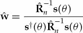
Using the method of Lagrange multipliers, the solution that maximizes the output SINR under the above-mentioned conditions is given by the closed-form expression in Eqn. (9.5), which is often referred to as the Capon optimum beamformer (Capon 1969).

(9.5)
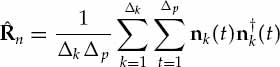
The interference-plus-noise spatial covariance matrix Rn is unknown a priori and needs to be estimated from the received data in practice. A popular method for estimating the optimum weight vector  is the sample matrix inverse (SMI) technique (Reed, Mallet, and Brennan 1974). This involves substitution of Rn in Eqn. (9.5) with the sample covariance matrix (SCM)
  in Eqn. (9.6). The SMI technique assumes the availability of training data nk (t) containing interference-plus-noise only. Ideally, these vectors are extracted from Δk ranges and Δp PRI not containing clutter or useful signals. A sufficient number of independent vectors ΔkΔp ≥ N is required to ensure that
  exists.
(9.6)
Although this may appear to be an ad hoc approach, the SMI technique has a number of very important properties. For a finite number of available training samples, the SMI method converges more rapidly to the optimal solution than gradient-descent estimation techniques such as the LMS algorithm, particularly when Rn is poorly conditioned due to the presence of powerful interference with low spatial rank. Moreover, when nk(t) is zero-mean complex Gaussian distributed, the SCM is the maximum likelihood (ML) estimate of Rn, and by the invariance principle,  in Eqn. (9.7) is the ML estimate of wopt.
(9.7)
Provided is computed using ΔkΔp > 2N statistically independent training vectors nk(t), the average loss in output SINR due to estimation errors in relative to wopt is less than 3 dB irrespective of the form of the interference-plus-noise spatial covariance matrix Rn (Reed, Mallet, and Brennan 1974). The results of Cheremisin (1982) and Abramovich (1981b) show that by appropriate diagonal loading of the sample covariance matrix, the number of independent snapshots required for less than 3 dB average losses in output SINR can under certain circumstances be reduced to 2Ne, where Ne < N is the interference subspace dimension. The introduction of diagonal loading with appropriate loading factor α in Eqn. (9.8) can therefore significantly improve convergence rate when sample support is limited.
(9.8)
9.2.2 Practical Implementation Schemes
Operational considerations affect how adaptive beamforming can be applied in practice. A key issue is that during normal operation an OTH radar system receives powerful clutter in addition to useful signals and interference. The presence of radar echoes in the training data needs to be avoided so as to effectively estimate the interference-plus-noise spatial covariance matrix Rn. One approach is to schedule a brief period of passive data collection prior to each active coherent processing interval (CPI). The clutter-free training data collected during this period is used to train the adaptive beamformer which is then applied to the CPI that follows.
Turning the transmitters off temporarily before each CPI represents a possible option. However, this method may not be advisable in certain practical systems due to the risk of damaging hardware. An alternative is to deliberately assign the transmitter to a different carrier frequency for a brief period, such that clutter returns are temporarily out of band and hence not received by the system during the interference-plus-noise sampling interval. This allows the transmitter to be driven continuously at a constant power.
The interference-plus-noise SCM is computed using array snapshots received during the “passive” training interval. This estimate is used to synthesize the adaptive beam-forming weight vector according to the SMI or diagonally loaded SMI technique. The resulting spatial filter is then used to process the entire CPI of operational data that immediately follows the interference-plus-noise sample train. The adaptive beamformer does not attempt to cancel clutter in the CPI. Clutter and useful signals can be separated into different frequency bins by Doppler processing after adaptive beamforming. The main role of adaptive beamforming is to reject the interference and pass on the useful signals. This procedure is repeated again to process the next CPI and so on in order to adaptively respond to changes in the spatial properties of the external interference-plus-noise environment.
Such a method is referred to as scheme 1 and has been illustrated in the upper left diagram of Figure 9.1. Assuming the spatial statistics of nk(t) are invariant across range over a relatively small number of Δp consecutive PRI, the received snapshots nk(t) for k = 1, …, Δk and t = 1, …, Δp may be regarded as different realizations of a locally stationary random process. These interference-plus-noise realizations may be considered independent, provided the interference bandwidth is larger or equal to the radar bandwidth and the receiver output is sampled at the Nyquist rate. The degree of independence among the different sample vectors in the training set will in general depend on the interference waveform characteristics as well as the window function used for pulse compression, which introduces correlation among neighboring range bins.
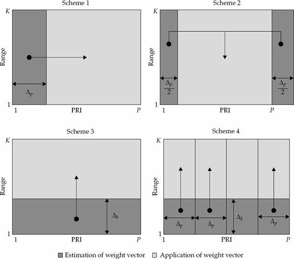
FIGURE 9.1 Conceptual illustration of the four adaptive beamforming schemes. Each diagram shows the range and PRI regions where the array snapshots are used to estimate the adaptive weight vector and the regions where the resulting spatial filter is applied to beamform the radar data. © Commonwealth of Australia 2011.
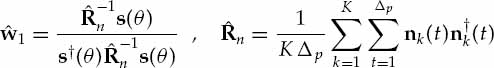
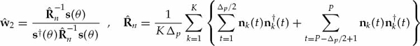
In scheme 1, the sample spatial covariance matrix  is formed using all available training data acquired during the “listening” period between the end of one CPI and the start of another. This training data is also commonly known as secondary data. The weights for adaptive beamforming scheme 1 are denoted by
  in Eqn. (9.9). In this case, the interference-plus-noise sample spatial covariance matrix is estimated using all processed range bins Δk = K over a subset of Δp consecutive PRI. The remaining PRI in the dwell (indexed by t = Δp + 1, Δp + 2, …, P) contain clutter and useful signals in addition to interference-plus-noise.
(9.9)
When the number of available snapshots K Δp is small, the performance of this method may be improved by appropriate diagonal loading of the covariance matrix  = + αI, and substituting for in Eqn. (9.9). The choice of α yielding the best performance is data-dependent. Typically, loading levels above the additive white noise power but well below the interference subspace eigenvalues provide best results. The beamformer output for scheme 1 is given by the scalar signal
  in Eqn. (9.10) for ranges k = 1, …, K and the operational set of PRI t = Δp + 1, Δp + 2, …, P.
(9.10)
When the spatial characteristics of the interference fluctuate over the CPI, a modification to scheme 1 that may improve performance is to average the sample spatial covariance matrices resulting at both ends of the CPI. The rationale behind this method, referred to as adaptive scheme 2 in Figure 9.1, is that variations of the interference-plus-noise within the CPI are better captured by a weight vector derived from the average of the two sample covariance matrices. The weight vector for this adaptive beamforming scheme is denoted as  in Eqn. (9.11), while the scalar output is given by
  for k = 1, …, K and t = Δp/2 + 1, …, P − Δp/2 with Δp assumed to be even.
(9.11)
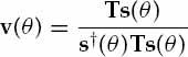
The matched filter beamformer is defined as N−1s(θ), where normalization by N provides unit gain in the beam steer direction, i.e., N−1s†(θ)s(θ) = 1. A real valued window function is often applied to reduce sidelobe levels. In this case, the mismatched conventional beamformer v(θ) may be written in the form of Eqn. (9.12), where the diagonal taper matrix T = diag[w1, …, wN] contains the window values  as its elements. Similar to adaptive schemes 1 and 2, the conventional beamformer in Eqn. (9.12) is also normalized to provide unit gain in the steer direction such that v†(θ)s(θ) = 1. The conventional output is given by yk(t) = v†(θ)xk(t).
(9.12)
As all the above-mentioned beamformers share the unit gain response to an ideal useful signal, the SINR improvements of schemes 1 and 2 relative to the conventional beamformer may be estimated as  and
and  , respectively, in Eqn. (9.13). In the case of passive mode data, we have that xk(t) = nk(t), so the quantities in Eqn. (9.13) represent the interference-plus-noise cancelation ratio. The two adaptive beamforming schemes described so far belong to a class of algorithms that we shall refer to as framing schemes.

(9.13)
An alternative method exploits the property that interference and noise are (normally) incoherent with the radar signal and will appear in all range cells processed, while clutter and useful signals often appear over a finite range extent that may only occupy a subset of the processed range cells. Specifically, clutter and useful signals are mainly present in a band of ranges beyond the skip-zone, where sky-wave signal propagation is supported by the ionosphere. Consequently, the signals received in the nearest range cells within the skip-zone, indexed by k = 1, 2, …, Δk < K, will be dominated by interference and noise. The skip-zone phenomenon allows the interference-plus-noise spatial covariance matrix to be estimated within the CPI, as illustrated in Figure 9.1. This alternative method is referred to as adaptive beamforming scheme 3. The weight vector for scheme 3 is calculated as  in Eqn. (9.14).
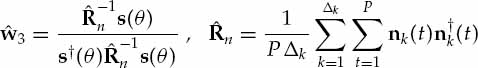
(9.14)
The scalar output and SINR improvement factor for scheme 3 are given in Eqn. (9.15). In this case, the operational data to be processed xk(t) are the set of range cells k = Δk + 1, …, K immediately beyond the skip-zone, which additionally contain clutter and potentially useful signals. The significant advantage of scheme 3 relative to framing schemes is that the adaptive beamforming weights are derived from an estimate of the interference-plus-noise spatial covariance matrix integrated over the CPI. The presence and number of skip-zone range cells depends on ionospheric conditions and the operating frequency. A potential drawback of scheme 3 is that such cells may not always be available in practice.

(9.15)
Experimental analysis of the relative improvement factors  enables the cancelation performance of different adaptive beamforming schemes to be compared. It is also of interest to determine whether the performance observed on real data can be accurately predicted by the HF channel simulator described in the previous chapter. For both these purposes, the statistical distribution of the quantities will be determined as a function of CPI length. In particular, the mean and deciles of these distributions will be calculated to provide an indication of cancelation performance for the different adaptive beamforming schemes.
9.2.3 Alternative Time-Varying Approach
The spatial structure of HF signals reflected by the ionosphere can vary appreciably over time scales commensurate with the duration of typical OTH radar CPI. However, it has been observed that changes in the signal wavefronts received from individual propagation modes are often highly correlated from one PRI to another. Stated another way, the received wavefronts tend to evolve in relatively smooth manner when viewed at a temporal resolution of less than one-tenth of a second.2 An HF signal mode reflected from a relatively stable and localized region of the ionosphere will therefore exhibit an almost steady spatial signature over a sufficiently short time interval comparable to the OTH radar PRI. The spatial covariance matrix of such a signal will therefore have a low rank when integrated over the “quasi-instantaneous” PRI. On the other hand, the spatial covariance matrix averaged over the relatively longer CPI converges to its statistically expected form, which may grow to full rank as the fluctuations of an angularly spread signal decorrelate in time.
It follows that forming the interference-plus-noise sample spatial covariance matrix over short time segments within the CPI provides a means to reduce the interference sub-space dimension and hence improve rejection performance. In other words, readjusting the antenna pattern a number of times within the CPI to adaptively “track” the spatial dynamics of the interference provides greater opportunity to reject such interference effectively. This capability becomes important when: (1) the number of independent interference sources and modes approaches the number of adaptive degrees of freedom, (2) the spatial properties of the interference wavefronts are changing rapidly, and (3) the CPI to be processed is long. In such situations, re-tuning of the adaptive weights a number of times within the CPI is likely to provide more effective interference cancelation.
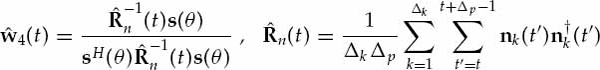
An apparently reasonable way of adapting the antenna pattern to the changing interference characteristics within the CPI is to form the slow-time varying SCM  using the skip-zone range cells integrated over a batch of Δp PRI starting at time t, and to calculate the adaptive weight vector
  in accordance with the well-known rule in Eqn. (9.16). The time-varying weight vector is then used to beamform the operational ranges cells
  for k = Δk + 1, Δk + 2, …, K in the current batch of PRI indexed by t, t + 1, …, t + Δp − 1. This time-varying method, referred to as adaptive scheme 4, is illustrated in Figure 9.1 for the case of non-overlapping batches.
(9.16)
Once the entire CPI of data is beamformed by the slow-time sequence of adaptive weight vectors, the scalar output needs to be Doppler processed to separate useful signals from the more powerful clutter returns. While the interference is expected to be rejected effectively by this approach, a serious problem arises due to the unwanted interaction between the intra-CPI antenna pattern fluctuations and the unrejected clutter returns that are passed onto the beamformer output. Specifically, the adaptive beampattern readjustments within the CPI temporally modulate the unrejected clutter returns in the beam-former output. This has the deleterious effect of broadening the clutter spectrum after Doppler processing. This operational issue, which can cause target echoes to be masked by clutter energy after Doppler processing, will be described in more detail later.
9.3 Instantaneous Performance Analysis
The interference rejection performance of different adaptive beamforming schemes may be quantified as a function of slow-time to observe how the instantaneous performance changes from one PRI to another within the CPI. Analysis of the instantaneous cancelation ratio sheds light on the intra-CPI performance of different adaptive beamforming schemes applied to interference reflected from the ionosphere. The main purpose of this analysis is to expose a number of important characteristics that are not predicted by simulation results based on traditional models.
9.3.1 Real-Data Collection
The collection of experimental data involved the passive reception of a cooperative HF interference source that radiated a bandlimited white signal. A vertically polarized omnidirectional (whip) antenna was used to emit this radio frequency interference (RFI) signal, which propagated via a one-hop mid-latitude ionospheric path to the Jindalee OTH radar receive system. The cooperative RFI source was located near Darwin in the far field of the 2.8-km long Jindalee receive antenna array. Specifically, the RFI source was at a ground range of 1265 km from the receiver site and offset +22 degrees from the ULA boresight direction. A clear 3 kHz bandwidth channel was exclusively allocated for the experiment at a carrier frequency of 16.050 MHz on 1 April 1998 between 06:22 and 06:32 UT.
It is noted that the channel scattering function (CSF) data analyzed in Chapters 6–8 corresponds to the same mid-latitude ionospheric path and was recorded on the same day immediately prior to this experiment (06:17–06:21 UT) on an adjacent frequency channel (16.110 MHz). The HF channel model parameters estimated from the CSF data are therefore relevant to those experienced by the interference in this experiment.
According to the real-time frequency management system (FMS), the operating frequencies used coincided with near optimum propagation conditions at the time of recording. Hence, experimental results based on this interference data are likely to estimate the impact of time-varying interference wavefront distortions on adaptive beam-former performance conservatively with respect to RFI sources propagated via disturbed ionospheric regions.
The bandlimited white noise signal acquired by the 32 receivers of the Jindalee ULA was observed to spread across the entire range-Doppler map in a significant number of beams after conventional processing. Each CPI consisted of P = 256 PRI and K = 42 range cells. Although a low PRF (of say 1 Hz) permits interference rejection to be studied over very long CPI (up to 256 seconds), it limits the shortest time interval over which the interference properties are integrated to a minimum of 1 second. On the other hand, increasing the PRF to say 50 Hz allows performance to be observed at a higher temporal resolution of 0.02 seconds, but limits the maximum CPI length that can be analyzed to around 4 seconds.
In this experiment, the selected PRF of 5 Hz represents a compromise between the two competing objectives, yielding a maximum CPI of 50 seconds and a temporal resolution of 0.2 seconds. Based on the previous CSF data analysis, the ionospheric channel under investigation is not expected to vary significantly within a PRI of 0.2 seconds. The RFI source was also switched off momentarily during the experiment in order to record background noise on the same frequency channel. This data serves as a reference to determine how effectively adaptive beamforming is able to reject the interference.
9.3.2 Intra-CPI Performance Analysis
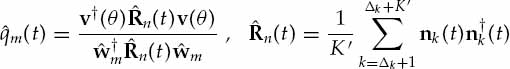
The SINR improvement factor  for m = 1, …, 4 in Eqn. (9.17) measures the relative output SINR improvement (RFI cancelation performance) of adaptive beamforming scheme m as a function of slow-time t. A Hamming taper was used for the conventional beamformer v(θ). Note that the instantaneous improvements are computed in K′ = 16 range cells taken after the first Δk = 16 “training” range cells in each PRI (i.e., cross-rejection as opposed to self-rejection).
(9.17)
The weights are formed using K = 32 and Δp = 6 in Eqn. (9.9). Curve 1 in Figure 9.2 shows  as a function of slow-time t over a 50 second CPI when the beam is steered at a cone angle of θ = 21.6 degrees (near the RFI source direction). This curve shows that the filter has a high initial effectiveness and yields 30 dB improvement relative to conventional beamforming close to the start of the CPI. However, this improvement drops rapidly and falls to below 5 dB in less than 2 seconds. After about 20 seconds, the filter “ages” to the point where conventional beamforming provides superior performance. More than 30 dB variation in performance is not expected under stationary conditions for an adaptive filter trained on K × Δp = 6N samples. In the traditional model, where the interference modes are assumed to have a time-invariant spatial structure, such a filter would be expected to provide near optimum performance over the whole CPI.
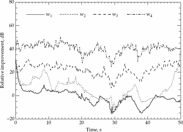
FIGURE 9.2 Relative performance improvements achieved by the four adaptive beamforming schemes as a function of PRI number over the CPI. © Commonwealth of Australia 2011.
The small-scale random variations of , possibly caused by finite sample effects, are superimposed on a relatively smooth large-scale variation that exhibits a physical (wavelike) characteristic between 20 and 50 seconds. These large-scale changes in rejection performance are not predicted by standard models and can only be attributed to variations in the interference spatial structure over the CPI. Based on this experimental result, it is evident that adaptive scheme 1 is quite ineffective for the purpose of sky-wave HF interference mitigation when the required CPI length exceeds approximately half a second.
Curve 2 in Figure 9.2 shows the results for  , where is formed according to Eqn. (9.11) using identical parameters as adaptive scheme 1 {K = 32, Δp = 6}. The same number of training vectors are used to estimate and . The range cells processed by and are also the same, so and can be meaningfully compared. Clearly, scheme 2 is a block processing algorithm that requires memory (data storage), whereas scheme 1 is a streaming technique that may be applied as the data is received. A comparison of curves 1 and 2 shows that scheme 2 performs better than scheme 1 over practically all of the CPI.
In particular, scheme 2 performs 20–30 dB better than scheme 1 in the final second of the CPI. This is expected because scheme 2 is based only on an estimate of the covariance matrix that averages the interference spatial statistics immediately before and after the CPI, whereas scheme 1 is based only on an estimate formed prior to the CPI. The performance of scheme 2 in the middle portion of CPI degrades by about 20 dB relative to that observed near the extremities. This is also expected because adaptive scheme 2 has no “knowledge” of the variations in RFI spatial structure over the middle region of the CPI. In general, the spatial properties of time-varying interference in this region of the CPI cannot be deduced or estimated accurately from data received outside the CPI.
Averaging the sample spatial covariance matrices estimated close to both ends of the CPI seems to provide a better estimate of the interference received within the CPI than using only the matrix formed prior to the CPI. This is evidenced by the 10 dB improvement of scheme 2 relative to scheme 1 in the middle region of the CPI. However, the results demonstrate that scheme 2 is also unsuitable for skywave HF interference mitigation in applications where the CPI length exceeds about 1 second. These observations strongly motivate the use of adaptive schemes that operate on estimates of the interference spatial covariance matrix formed within the CPI, such as adaptive scheme 3.
Curve 3 in Figure 9.2 shows the relative improvement  for adaptive scheme 3. The adaptive weight vector in Eqn. (9.14) is estimated using Δk = 16 training ranges using the sample covariance matrix averaged over the entire CPI, i.e., integrated over all P PRI. The resulting time-invariant spatial filter is then used to process the “operational” range cells k = Δk + 1, …, Δk + K′ in each PRI using K′ = 16 as before. Unlike the framing schemes, adaptive scheme 3 is based on an estimate of the interference spatial covariance matrix averaged during the CPI to be processed.
The performance of scheme 3 is observed to be 15–20 dB better than scheme 2 over almost all of the CPI. This approach may be quite effective for skywave HF interference mitigation, particularly in aircraft detection OTH radar applications that use a relatively short CPI. However, for a long CPI (e.g. ship detection), or when the interference fluctuations are rapid due to disturbed ionospheric propagation, scheme 3 may not be able to reject the interference effectively.
A remaining option to mitigate against interference spatial structure fluctuations is to update the weight vector within the CPI. Curve 4 in Figure 9.2 shows the improvement  corresponding to the slow-time varying weight vector . This sequence of spatial filters is computed using Eqn. (9.16), where Δk = 16 training cells are used in non-overlapping sub-CPIs each containing Δp = 4 PRI. A substantial performance gain in the order of 30–40 dB relative to the conventional beamformer results for scheme 4. A comparison between the time-invariant solution (curve 3) and the time-varying solution (curve 4) demonstrates that re-adapting the weights during the CPI yields an additional 15–20 dB of interference cancelation. It will be shown later that scheme 4 rejects the interference to the background noise floor.
The spatial processors and are clearly of the same dimension N = 16, but the number of adaptive degrees of freedom required for effective HF interference rejection tends to grow as the integration time increases. This is primarily caused by the time-varying wavefront distortions imparted on the received interference modes by the ionospheric reflection process. As these distortions evolve in a correlated manner over time, limiting the integration time serves to reduce the effective dimension of the interference subspace. This often allows an adaptive beamformer to cancel the interference more effectively. Exceptions to this may arise in the special case of main beam interference or when the RFI is propagated by the much more stable surface-wave mode.
Figure 9.3, in the same format as Figure 9.2, shows analogous results for a subsequent CPI of data. In this example, the beam steer cone angle of θ = 20.8 degrees is slightly further away from the direction of the RFI source. Although the corresponding curves differ in detail, the qualitative characteristics of the four curves in Figure 9.3 are similar to those of Figure 9.2. To quantify this variability, the statistical performance of the four schemes needs to be evaluated over different beam steer directions and CPI by extended data processing. An estimate of the average or expected performance can then be provided for the different adaptive beamforming schemes as a function of CPI length.
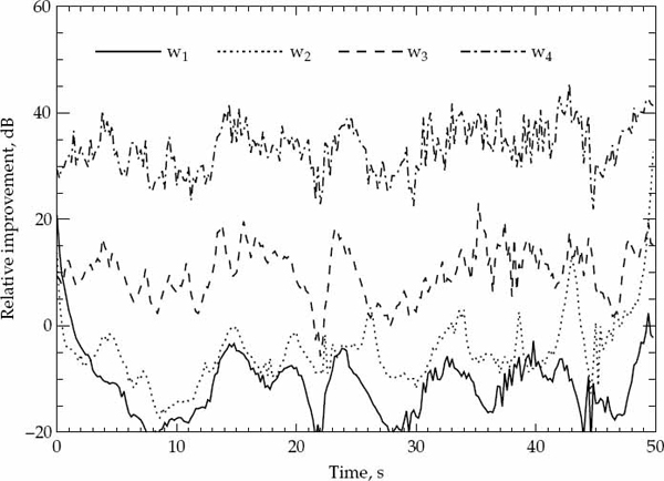
FIGURE 9.3 Relative performance improvements for the same adaptive schemes using a different CPI and beam steer direction. © Commonwealth of Australia 2011.
9.3.3 Output SINR Improvement
Before proceeding to the statistical performance analysis, the question arises as to whether adaptive scheme 4 rejects the interference to the background noise level. To answer this question, consider the Doppler spectra in Figure 9.4. Curves 1 and 3 show the Doppler spectra resulting for the conventional beamformer when the interference is present and absent, respectively. An ideal synthetic target has been injected with a normalized Doppler frequency of 0.5 in both cases. The target is clearly visible when only background noise is present (curve 3). Note that this is actual background noise recorded at the same frequency as the interference source when the latter was switched off during the experiment. When the interference is additionally present (curve 1), the target is submerged and cannot be detected in the conventional beamformer output.

FIGURE 9.4 Conventional Doppler spectra for a simulated target signal in real HF interference (curve 1) and real background noise (curve 3). Curve 2 shows the Doppler spectra resulting when adaptive scheme 4 is applied with interference present. © Commonwealth of Australia 2011.
Curve 2 in Figure 9.4 shows the Doppler spectrum resulting at the output of adaptive scheme 4 when the interference is present. In this case, the adaptive weights w4(t) were updated from one PRI to another over the CPI with diagonal loading to improve convergence. The slow-time varying weight vectors were then applied to beamform the range cell containing the synthetic target, which was not included in the training data. A comparison of curves 1 and 2 in Figure 9.4 demonstrates that re-adapting the antenna pattern within the CPI attenuates the interference by an additional 40 dB relative to the conventional beamformer.
It is evident from curves 2 and 3 in Figure 9.4 that both adaptive and conventional beamformers provide identical response to the target echo. This demonstrates the equivalence between interference cancelation ratio and relative SINR improvement for the considered schemes assuming ideal useful signals. The cancelation ratio translates to an SINR improvement provided the ideal useful signal is not included in the training data. Importantly, curves 2 and 3 also demonstrate that adaptive scheme 4 has practically rejected the interference to the background noise level. Application of scheme 4 therefore has the potential to restore the output SINR to that of the conventional beamformer on a clear frequency channel. From an interference rejection and ideal signal reception viewpoint, the performance of adaptive scheme 4 is as good as can be.
9.4 Statistical Performance Analysis
The previous results illustrated a number of key points in detail, but a more comprehensive performance analysis is required to quantify the relative merits and shortcomings of the different adaptive beamforming schemes. As the relative improvement factors  are random variables, it is of interest to measure the mean and upper/lower deciles of their distributions as a function of CPI length by analyzing more data.
9.4.1 Framing Schemes
Figure 9.5 shows the mean and deciles of the distribution of for a number of different CPI lengths. For each interrogated CPI length, a total of 10 mutually orthogonal beam steer directions were processed in 40 different CPIs such that the distribution for each CPI length is based on 400 samples of the improvement factor. Figure 9.5 demonstrates that the mean relative improvement drops from above 30 dB to below 0 dB as the CPI is increased from a fraction of a second to 40 seconds. The fall in performance of adaptive scheme 1 is observed to be very rapid, as over 20 dB of interference rejection is on average lost in less than 2 seconds. The higher computational load of adaptive scheme 1 relative to conventional beamforming is therefore not warranted for OTH radar applications according to these experimental results.
FIGURE 9.5 Mean and deciles of the improvement in interference rejection performance achieved by adaptive scheme 1 () over the conventional beamformer as a function of CPI length. © Commonwealth of Australia 2011.
Figure 9.6, in the same format as Figure 9.5, shows the mean and deciles of to determine the performance of adaptive scheme 2. The mean relative improvement is above 40 dB for very short CPI, but decays to 25 dB after only two seconds and then down to almost 0 dB when the CPI reaches 30 seconds. Although the performance of scheme 2 decays less rapidly compared to that of scheme 1, the significant performance degradation for CPI lengths greater than about 2 seconds may not be tolerable when powerful interference is present. Based on these experimental results, it is evident that scheme 2 may also not perform sufficiently well in practice to justify operational implementation.

FIGURE 9.6 Mean and deciles of the improvement in interference rejection performance achieved by adaptive scheme 2 () over the conventional beamformer as a function of CPI length. © Commonwealth of Australia 2011.
9.4.2 Batch Schemes
Figure 9.7 shows the mean and deciles of the improvement factor  for scheme 3. The maximum mean value of about 43 dB occurs at a CPI length slightly above 1 second. A degradation of up to 8 dB is observed for shorter CPI due to estimation errors caused by finite sample support. While for longer CPI lengths, the degradation is caused by fluctuations in interference spatial structure. Hence, the best performance for scheme 3 occurs at a CPI length that provides an optimal tradeoff between convergence losses due to finite sample support at very short CPI, and dynamic losses caused by interference fluctuations at longer CPI. Adaptive scheme 3 provides quite acceptable performance for CPI lengths shorter than about 4 seconds in the analyzed data set.
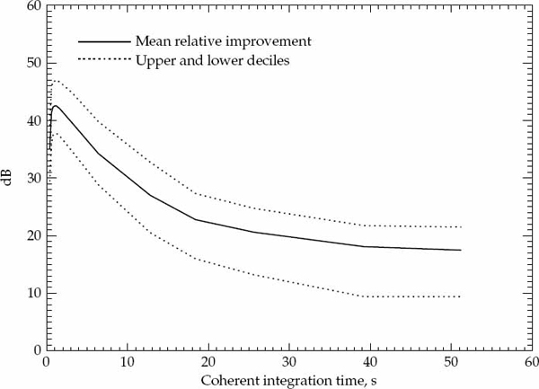
FIGURE 9.7 Mean and deciles of the improvement in interference rejection performance achieved by adaptive scheme 3 () over the conventional beamformer as a function of CPI length. © Commonwealth of Australia 2011.
Moreover, diagonal loading can be applied to reduce losses due to limited training data. This is illustrated in Figure 9.8, where the statistics have been recalculated using a loading factor of −20 dB (α = 0.01). This simple modification increases the mean relative SINR improvement from 35 to 45 dB for CPIs under a second, a remarkable 10 dB increase with respect to the case where no loading is applied. However, the 10 dB performance degradation observed for adaptive scheme 3 as the CPI increases from 1 to 8 seconds cannot be recovered as this is caused by fluctuations of the interference spatial structure. The more significant performance degradation of around 25 dB for CPI approaching 50 seconds also poses a problem in OTH radar applications that require high Doppler resolution.

FIGURE 9.8 Mean and deciles of the improvement in interference rejection performance achieved by adaptive scheme 3 after diagonal loading relative to the conventional beamformer as a function of CPI length. © Commonwealth of Australia 2011.
For this reason it is of interest to determine the potential effectiveness of scheme 4, which adjusts the spatial filter to process the data in batches consisting of relatively few consecutive PRI. The performance of adaptive scheme 4 can also be inferred from Figure 9.7, since every batch of PRI may be considered as a sub-CPI of the total CPI. In other words, if the adaptive weights are updated every second using scheme 4, the mean relative improvement of about 43 dB observed for this update rate in Figure 9.7 can be attained for a CPI that is arbitrarily longer. For example, 43 dB of additional interference cancelation relative to the conventional beamformer could be obtained for a CPI of 50 seconds because the performance of adaptive scheme 4 is determined by the batch length as opposed to the CPI length.
9.4.3 Operational Issues
In relation to adaptive scheme 4, the main operational issue relates to the application of a time-varying array weight vector to a CPI of data that also contains clutter. Due to the relatively broad angular coverage of the OTH radar transmit beam, the clutter has a spatially wideband characteristic as the backscatter is incident from a continuum of directions that occupy a significant portion of the receive antenna radiation pattern. Unconstrained fluctuations of the receive antenna pattern during the CPI imposes a temporal modulation on the output clutter signal that causes it to spread across the target velocity search space after Doppler processing.3 This issue represents the main impediment to the practical application of scheme 4.
Hence, the problem faced is to not only allow adaptive beampattern readjustments within the CPI to enhance interference rejection, but also to simultaneously control these variations so as to preserve the temporal correlation properties of the backscattered clutter at the beamformer output. Alternative approaches that address this problem are described in the next chapter. Other operational issues that can potentially limit performance include the lack of clutter-free training data and mismatches between the useful signal structure and the presumed steering vector model. These issues will also be discussed in the following chapter. Clearly, the computational complexity of scheme 4 is higher than those of schemes 1 to 3. This may limit scope for real-time implementation. Trading off batch length with performance represents an option to reduce the computational complexity of scheme 4.
9.5 Simulated Performance Prediction
The space-time HF channel model described in the previous chapter may be used to simulate the statistical characteristics of the interference received by the Jindalee antenna array. The temporal parameters of the HF channel model cannot be estimated from the interference because this signal is not coherent with the radar waveform. However, the interference was received over the same propagation path at a similar time and frequency to the channel scattering function (CSF) data analyzed in Chapters 6–8. The channel parameters estimated from the CSF data may therefore be used to simulate the interference. The capability of the HF channel model to predict adaptive beamformer performance results observed on experimental data can then be assessed.
9.5.1 Multi-Channel Model Parameters
The model parameters used for the simulation are listed in Table 9.1. The relative power ratios among the different interference modes are assumed to be the same as those of the CSF data modes, but scaled up in absolute power such that the total power of the modeled interference equals the total power measured for the actual interference received by the system. The received interference power was estimated by calculating the mean square value of the data in each receiver over the data collection interval and then averaging these results over the different receivers. The average power of the received interference was 30.2 dB.

TABLE 9.1 Interference simulation parameters assuming five propagation modes and the HF channel model estimated from the channel scattering function data. The constants are k1 = 2π/fp where fp = 5 Hz and k2 = 2πΔd/λ, where Δd = 84 m, λ = c/fc = 18.7 m, and the subarray steer direction θs = 22.0 degrees.
Note that the mode powers listed in Table 9.1 are not equal to the mode interference-to-noise ratios (INR), since the background noise level is at approximately −27 dB when measured in a single receiver prior to Doppler processing. The mode INRs can be therefore be calculated by adding 27 dB to the powers listed in Table 9.1. The noise added to the simulated interference is real background noise recorded on the same frequency channel in the absence of interference. Further aspects that need to be addressed in the simulation are the generation of the interference mode waveforms gk (t − τm) with time delays τm, and the correlation among the different modes.
The interference signal has a bandwidth of fb = 3 kHz with a relatively uniform power spectral density. The temporal auto-correlation sequence of the interference waveform is a sinc function with the first null at time delay τ = 1/fb = 0.33 ms. As the differential mode time-delays are known from the oblique incidence ionogram recorded for the CSF data analysis, each pair of modes can be assigned an inter-mode correlation coefficient according to the interference auto-correlation function. These correlation coefficients ρi, j for all pairs of modes i, j = 1, 2, …, M = 5 are entered into the source covariance matrix Rs in Eqn. (9.18), where the diagonal elements of Rs are unity as the mode waveforms gk(t − τm) are normalized to unit variance by definition in the model.
(9.18)
Once the source covariance matrix has been determined, the interference mode waveforms can be generated simultaneously using Eqn. (9.19), where  is the Hermitian square root of the source covariance matrix. The statistical independence of the zero-mean complex Gaussian vectors nk(t) over range k and slow-time t implies that the interference samples generated for a particular mode are white and hence uncorrelated in both of these data dimensions.
(9.19)
9.5.2 Impact of Wavefront Distortions
In the traditional array-processing model, the interference wavefronts are assumed to remain rigid over the CPI. The absence of time-varying wavefront distortions on the received interference modes implies that the spatial poles of the model lie on the unit circle. It is therefore possible to revert to the traditional model by setting the magnitude of the spatial pole estimated for each interference mode in Table 9.1 to unity. In this case, the interference modes are modeled as plane waves with Doppler shifted and Doppler spread waveforms due to temporal channel fluctuations only. Based on this model, Figure 9.9 shows the mean and deciles of the improvement factor when the simulated data is processed in identical manner to real data results shown in Figure 9.8.

FIGURE 9.9 Relative improvement achieved by adaptive scheme 3 (after diagonal loading) for simulated HF interference with temporal distortions but in the absence of spatial distortions. © Commonwealth of Australia 2011.
As the spatial structure of each interference mode is assumed to be time-invariant in the traditional model, the dimension of the interference subspace cannot increase beyond M = 5 regardless of the CPI length. This explains why the mean relative improvement in Figure 9.9 remains approximately constant with increasing CPI length. Diagonal loading has been applied here as it was for Figure 9.8. Clearly, the traditional plane wave interference model does not provide an acceptable representation of the experimental results in Figure 9.8. The substantial difference between Figures 9.8 and 9.9 illustrate that results based on this model are of limited value for OTH radar systems, as they do not provide an accurate indication of practical performance in the HF environment.
Figure 9.10 shows the recomputed statistics for after the time-varying interference wavefront distortions are introduced using the model parameters in Table 9.1. The simulation results in Figure 9.10 show that the mean relative improvement drops from 46 dB for a CPI length of less than 1 second to 18 dB for a CPI of about 50 seconds. This agrees well with the experimental results in Figure 9.8, which report a drop in mean performance from 45 dB to 17 dB over the same range of CPI lengths. The detailed shapes of the curves in Figure 9.8 and Figure 9.10 are clearly not the same, but the described HF channel model and estimated parameters provide a quite accurate description of adaptive beamformer performance in the HF environment. A similar experiment demonstrating the close agreement between simulated and experimental performance results for adaptive beamforming scheme 1 using different CSF and interference data sets can be found in Fabrizio et al. (1998).

FIGURE 9.10 Relative improvement achieved by adaptive scheme 3 (after diagonal loading) for simulated HF interference with the inclusion of space-time distortions. © Commonwealth of Australia 2011.
9.5.3 Summary and Discussion
The presence and characteristics of wavefront distortions imparted on HF signal modes reflected by the ionosphere were confirmed, analyzed, and modeled in Chapters 6–8. This case study quantified the operational impact of such phenomena on the performance of four standard adaptive beamforming schemes applied to the problem of interference rejection in OTH radar systems. As opposed to useful signals, which are received in the relatively broad main lobe of the beam pattern, interference is typically received near the deep “nulls” of an adaptive antenna pattern, where the array response is much more sensitive to time-varying wavefront distortions. The first important observation is that dynamic wavefront distortions imparted on interference signal modes have the potential to dramatically degrade the rejection performance of HF systems when time-invariant adaptive beamforming schemes are used to process each CPI.
Second, it has been shown that traditional array signal-processing models poorly represent adaptive beamformer performance in the HF environment. Such models are therefore not suitable for guiding algorithm design or predicting practical performance in OTH radar systems. For applications that require high fidelity, it was also shown that the previously validated HF channel model could be used to simulate HF interference signals received by a very wide aperture antenna array and accurately predict the statistical performance of an adaptive beamformer as a function of CPI length.
The final observation is that the presence of time-varying interference wavefront distortions needs to be accounted for in order to develop effective adaptive beamforming algorithms for operational OTH radar systems. In particular, methods that can stabilize the Doppler spectrum characteristics of the backscattered clutter signals when the adaptive beamforming weights change several times during the CPI to ensure effective interference rejection are required. Without such methods, the potential benefits of updating the spatial filter within the CPI cannot be realized in practice. This motivates the search for alternative adaptive beamforming techniques suitable for real-time implementation in OTH radar.
____________________
1 Methods for allocation of adaptive degrees of freedom are suggested in Steinhardt and Van Veen (1989).
2 This applies for single-hop propagation over a relatively quiet mid-latitude ionospheric path.
3 Recall that the response of the adaptive antenna pattern is only constrained in the beam steer direction, where the array provides fixed unity gain response to ideal useful signals. In other directions, the response of the receive antenna pattern is unconstrained for the adaptive schemes considered.
..................Content has been hidden....................
You can't read the all page of ebook, please click here login for view all page.