
CHAPTER |
|
19 |
Animating Items on the Map |
If you have read the book so far, you’re ready to tackle all types of mapping projects. You can annotate maps with markers and shapes and enable users to edit these items interactively. You can also publish your finished maps and save the annotations to KML files. In the last two chapters of this book, you will learn about another exciting feature of mapping applications: namely, how to animate items on the map. This chapter isn’t about bouncing a few happy faces on your map, or making a label drop in place. I’m talking about real animation of map items, such as moving the symbol of a train on its track in real time, or the symbol of an airplane along its flight path.
The techniques for animating items on the map are not part of the Google Maps API. As you will see shortly, it’s a feature of the JavaScript language and it’s implemented with a few functions. The sample applications you’re going to build in this chapter demonstrate the use of JavaScript’s animation functions and apply them to Google Maps objects, mostly for animating symbols along fixed paths, but also for animating attributes such as the transparency of a circle, the density of a heatmap, and any quantity that has a temporal component. The preceding chapters focused on the spatial aspect of data, so now we'll combine the spatial and temporal dimensions of data. A list of cities and their populations or their temperature is a dataset with a spatial component and you know how to present this component on the map. The same list with data for several years has a temporal dimension too, and the only way to visualize this dimension is to generate an animation that evolves with time.
Animating Items on a Map
The most interesting samples you’ll examine in this chapter are based on symbol animation, such as moving the symbol of an airplane along its flight path, or the symbol of a train along its track. As you recall from Chapter 8, it is possible to place one or more instances of a symbol along a
Polyline object. You know how to repeat a symbol along the line to indicate the flow of movement or other relevant information. The symbols can be placed at specific intervals along the line and these intervals can be expressed either in pixels or as percentages of the path’s total length. Figure 19-1 shows the geodesic path between two airports that are far away from one another. The symbol of an airplane is repeated along the line to indicate that the line is a flight path. The symbols of this specific figure (which is a repeat of Figure 10-2 from Chapter 10) are repeated every 50 pixels along the underlying path. Note that the path on which the symbols are placed is made transparent, and only the airplane symbols are visible on the map. The figure was generated by the Geodesics with Symbols.html sample page, included in the chapter’s support material.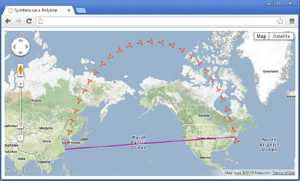
Figure 19-1 Using symbols to create alternative paths on a map
The idea behind animating a symbol is to place a single symbol at the beginning of a path and change its relative position every so often. For example, you can animate an airplane symbol along its flight path by setting its initial position to 0 percent of the path’s length and increasing the percentage by 100/60, or 1.66 percent, every second. The symbol will move from the departure airport to the destination airport in 60 seconds. If that’s too slow for your animation’s purposes, shorten the animation cycle (move the symbol every half a second, or less) or double the increment (advance its position by 3.3 percent of the total length at a time). In general, you should use a shorter animation cycle to speed up the animation. If things move by leaps, then the animation becomes “bumpy” and “jerky.”
There are other types of items you can animate on a map. It’s also common to animate object attributes, such as the size, color, or transparency of a Circle object. You can make a filled circle appear gradually on a map by changing its opacity in small steps. You will see an example of attribute animation in the following chapter.
Basic Animation Concepts
The two basic components of the animation are (a) a function that implements the animation, known as the animation function, by changing the position of an item, or one of its attributes and (b) the interval between successive invocations of the animation function. The animation function contains a block of statements that update the contents of the web page to produce the animation. The interval between successive invocations of the animation function is known as the animation cycle. It goes without saying that the animation function should complete in a single animation cycle. Otherwise, some animation steps will be skipped and the animation will not be as smooth as you’d expect.
The statements that are executed in every cycle handle the animation itself: They redraw the items on the map at their new locations. To produce any type of animation, you redraw the same image with small changes many times per second. When the changes are played back in rapid succession, the human eye can’t distinguish the various frames, and animation appears to evolve smoothly.
Animating in JavaScript is performed in real time: The animation function does all the calculations in real time and redraws the animated items on the map in rapid succession. You don’t have the luxury to create animation frames offline and play them back later. Instead, you must produce optimized code that can be executed many times per second. Today’s fast processors and GPUs (Graphics Processing Unit) support are a big help, but it’s of the utmost importance that your code is very efficient.
JavaScript Animation
To animate items on a Google Map, you need a single and surprisingly simple method, the
setInterval() method. This method, which belongs to the window object, accepts two arguments: the name of the animation function and the animation cycle in milliseconds. Every time this interval elapses, the animation function is executed. The following call to the setInterval() function call will cause whatever function you specify with the first argument to repeat every 500 milliseconds.The
setInterval() function returns an integer, which identifies the specific animation. You use this integer for a single purpose: namely, to end the animation with the clearInterval() method, which accepts as argument the identifier of an animation started with a call to the setInterval() function. animation_function is the name of the animation function. You can also define this function inline, in which case the call to the setInterval() method looks like this:
The
setInterval() method is called once, but the function you specify as its argument will be executed indefinitely, unless you stop it with a call to the clearInterval() method. The two functions are not used exclusively for animation; in fact, they weren’t even included in the language for this purpose. The setInterval() method enables a script running at the client to repeat a task every so often, and this task is usually to contact a remote server to retrieve data such as stock prices, real-time measurements, and other timely information. The web page can be updated automatically from within the script when changes in the remote data occur, without any user interaction.Figure 19-2 shows a very simple fiddle that demonstrates how the
setInterval() function is used. The page’s script displays the value of a variable, count, which is increased every 1.5 seconds. When the variable reaches its maximum value, 10, the script stops calling the function specified in the call to the setInterval() function. The script shown in Figure 19-1 is shown next: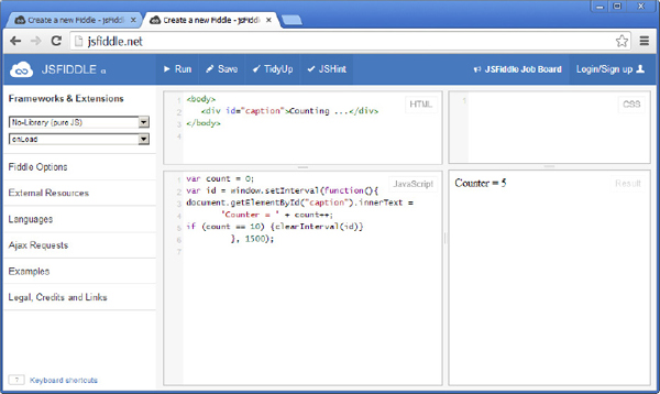
Figure 19-2 A simple script that demonstrates the use of the
setInterval() and clearInterval() methods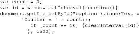
Using the
setInterval() method to perform animation is practically just as simple: Instead of updating the contents of a <div> element, you change the position (or the shape) of an item on the page. You can change the location of a marker or label on the map, the radius of a circle, and so on. In the examples of this chapter, you will change the position of a symbol along a path on the map.The Paris Metro Animated
In the remainder of this chapter, and in the following one, you will build some interesting animation applications. This section’s sample application involves one of the largest subway systems in the world, the Paris Metro. You’re going to develop a web page that displays the lines of the Paris Metro, along with their stations, and animates a train on each track. You will actually see a number of trains (depicted with small discs) move back and forth on their tracks.
The
Paris Metro.html web page is shown in Figure 19-3. The colored discs along each line are the line’s stations and the white discs (only one per line) are the moving trains. Each line in the Paris metro map has its own color, in addition to a name, and the actual colors were used for the lines and their stations—the saturation may be wrong, but you get the idea. Open the application and click the Animate Trains buttons to see the animation in action. The map is a bit dark because I’ve overlaid a semitransparent layer to smooth out the sharper features of the map and help the viewer focus on the metro lines, instead of the map elements, street names, and so on. You can remove this layer, if you wish, or experiment with custom map styles to simplify the background and bring forth the items of interest, which are the metro lines and their stations. For information on styling your maps, see Appendix C available online.
Figure 19-3 Each line of the Paris Metro is represented by a colored line. The metro stations are shown as solid circles, while the moving trains are shown as white circles.
The trains start all at once and travel at the same speed toward their destinations. As each train reaches its terminal station, it reverses its direction and starts traveling toward the terminal station at the other end of the line, and so on. The application uses an average speed, which includes the time at the stations. You can experiment with different train speeds, and you can even include a stop time at each station. This last feature, however, requires a bit of extra code and, although far from trivial, it would make a very interesting project.
Figure 19-4 is a detail of the Paris Metro web application and it shows the names of the stations along the blue line. To view the stations along a line, just pick the line on the map with the mouse. The selected line is rendered in white color to stand out and the names of the stations are shown as labels on the map. As you have probably recognized, the labels are implemented with RichMarker objects, an object that was discussed in detail in Chapter 7. Another useful feature you can add to the application is the ability to display the name of the next station of the selected line on a separate element of the page. Each time the train of the selected line reaches a station, you could display the name of the next station on the form. Short of zooming and dragging the map, the selection of a line is the only custom user interaction feature of the application. No action takes place when the user clicks a metro station, or the station’s label.

Figure 19-4 When you select a Metro line, the application displays the names of the stations along the selected line.
The image was captured 27 minutes and 45 seconds after the animation was started. This time interval corresponds to 1 hour and 59 minutes of actual travel time. In other words, 7,140 seconds of actual travel time (1 × 3600 + 59 × 60) were scaled down to 1665 seconds, which is equivalent to a scaling factor of approximately 4.3. In other words, 1 minute of real time is condensed into 14 seconds of animation time (scaled time), which is a reasonable scaling factor for this type of application. As you will see, an important aspect of any practical animation is to scale the speed of moving objects and keep track of the elapsed time. In the following sections, you learn how to design animations that simulate real-world scenarios, like the movement of trains and airplanes.
The Application’s Data
Before you explore the application’s code, you should take a look at the structure of the data used for the metro lines and how the data was obtained. Because I didn’t have access to the actual coordinates of the Paris Metro's tracks, I used the Map Traces application of Chapter 9 to generate a list of named locations (the stations) and their coordinates. If you live in Paris, you will probably spot some errors in the data; even so, bear with us through the code’s explanation. If you come up with a more accurate or more elegant application, please share it. The names of each line’s stations came from Wikipedia; then the stations were located on the map by their names and used as guides to trace the metro lines. As you can see, the tracks take very sharp turns at the stations, making it rather obvious that each path was constructed with consecutive line segments.
As you recall from Chapter 9, the Map Traces application is a map-driven Windows application. Its interface is repeated in Figure 19-5 for your convenience. This application allows you to trace any route on the map and saves the coordinates and names of its vertices to a KML file. The KML file generated by the Map Traces application was then converted manually into an array of JSON objects and embedded into the application’s script. If you’re interested in this or any other metro system, you can use this application and other sources of information, such as Wikipedia, to trace any path based on map features.
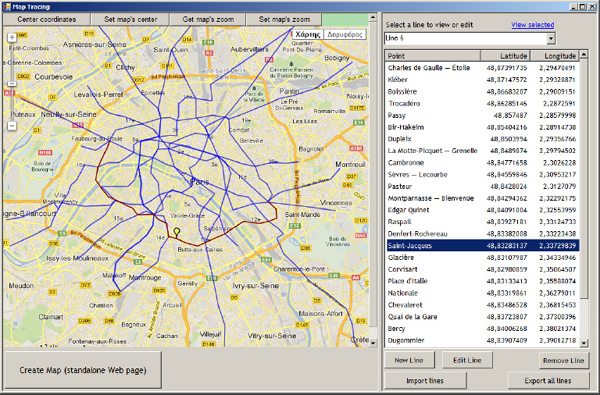
Figure 19-5 Tracing the routes of the metro line on the map with the map tracing application. The figure shows the trace of Line 6 with the Saint-Jacques station selected both in the list and on the map.
The “Floating” Stations
Some rather unexpected problems were encountered during the tracing of the paths of the Paris Metro lines, as demonstrated in Figure 19-6. I mention it here because it can totally confuse you and make you think you’re not using the application correctly, or that the application behaves strangely. The problem is demonstrated with Google Maps and not by the application itself. Both maps shown in the figure are centered near the Mabillon metro station. The map on the left was captured at a zoom level of 16 and the station is shown between Rue du Four and Boulevard Saint-Germain. The map on the right was captured at zoom level 17, and this time the same station is south of Rue du Four! This is a side effect of the tile mechanism used by Google to serve sections of the map. The titles are different at different zoom levels, as they contain different levels of detail. This is an extreme example of things that can go wrong. You should trace the features you’re interested in at the deepest possible zoom level, even if they are not in total agreement with the map at other zoom levels. If you examine the image carefully, or if you look up this part of the world in Google Maps, you will also notice that the other metro station (Saint-Germain-des-Pres) is not at the same location at all zoom levels. The metro lines that stop at these stations will not always appear to go through the station; at some zoom levels, the lines will appear to go near the stations, but not right over the stations.
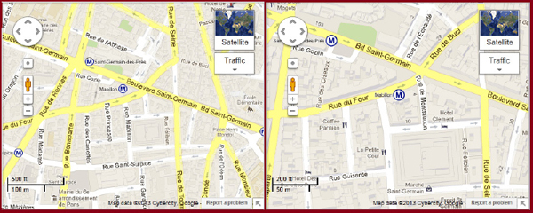
Figure 19-6 The location of the Mabillon metro station on Google Maps is slightly different at different zoom levels.
The Array with the Metro Data The application’s data are the locations of the stations that make up the paths of the metro lines; this data must be downloaded to the client as part of the script. You can request the data from a remote server as needed with a web service, but this specific application needs the data at the client at the same time. Because the script requires all data at the client, and because the paths of the metro lines aren’t likely to change, you can include the data in your script or store it to a JavaScript file at the server and include this file in your script. The application uses an array of custom objects to embed the metro lines and their stations into the script. The metro lines and their stations are stored in an array of custom objects with the following structure:
where
line is the name of the metro line, color is the color of the metro line, and stations is an array of custom objects, one for each station. Each station is stored in a custom object with the following structure:where
name is the station’s name and coords is a LatLng object with the station’s geo-coordinates. Here’s an object that represents a station:The data is stored in the
Paris_Metro array, whose contents are shown in Listing 19-1 (just a small section of the lines and their stations; you can open the Paris Metro.html page to examine the entire contents of the Paris_Metro array).Listing 19-1 The structure and contents of the
Paris_Metro array
Embedding the JSON formatted data into your script is straightforward. Just make sure you escape any special characters such as the single quote (see the last station’s name in the preceding listing). The
Paris_Metro array contains custom objects, and each custom object has a property—the stations property—which is also an array of custom objects with a different structure.TIP Some of the stations may end up being stored in multiple arrays. These are the stations where multiple metro lines merge. A more elegant approach would be to store all stations in a single array and associate an
id value with each station. Each metro line then would be a sequence of ids that correspond to the stations along the line. With this technique, you wouldn’t have to store the same station more than once, even if it’s shared by multiple metro lines. This approach would complicate the code and would have made it more difficult to follow.Designing the Metro Map
With the data in place, you can examine the code that draws the metro lines on the map and animates the trains. Each metro line is rendered on the map with a
Polyline object, which is defined by a path. The vertices of the path are the locations of the stations of the corresponding metro line. By the way, the actual subway rails are not straight-line segments between the stations, but unless you have access to more detailed data, there’s not much you can do. If the rails were on the surface of the city, you would be able to trace them more accurately by using many more points along each line. The animation techniques explained in this chapter, however, can be easily applied to any other path.To draw each metro line on the map, you must set up two nested loops: one that iterates through the lines of the
Paris_Metro array and another one that iterates through the current line’s stations. For each line, you must construct an array of coordinates and then use it as the path for a Polyline object that represents the current metro line. In the inner loop, you must also create a Circle object for each station and place it on the map at the station’s location. Listing 19-2 shows the two nested loops.Listing 19-2 Laying out the metro Lines and their stations on the map

The code stores the coordinates of the current line’s stations in the
path array—a local variable—and uses this array to specify the path of the Polyline object that represents the current metro line on the map. The following statement adds to the path array the location of the current station of the current line:The
path array is used later by the statement that creates the Polyline object corresponding to the current metro line: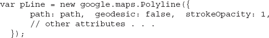
The
Polyline objects that represent the metro lines are stored in the lines array so that they can be reused later during the animation. The last statement in the listing associates each line’s click event with the selectLine() function, which highlights the line that was clicked.Designing the Animation
The trains travel on their paths at a constant speed and the application assumes the same speed for all trains, which is a reasonable assumption, but in a different type of application you could use a different speed for each moving object. Once you know the speed of the train and the length of the line, you can calculate the percentage of the line’s length covered at each animation cycle. Let’s say that the animation cycle specified in the
setInterval() function is 1000 milliseconds, which is 1 second, and the line’s length is 18 kilometers. The position of the train is updated once every second. If the speed is 36 kilometers per hour, it will take 30 minutes for the train to travel the distance. This will result in a very slow animation so you must speed things up by varying the animation time.Let’s do the math. The speed of the train is 36,000 meters per hour, or 36,000/60 = 600 meters per minute, or 600/60 = 10 meters per second. The entire distance is 18,000 meters and it will be covered in 18,000/10 = 1,800 steps. Between successive animation steps, you must advance the train’s symbol by 1/1,800 of the total distance, which is 18,000/1,800 = 10 meters. In real time, the entire length of the line will be covered after 1,800 seconds, or 30 minutes. Initially, the train’s position will be at the starting position, or 0 percent of the total length away from its starting position. After the first animation cycle, the train’s position will be at 10/18,000 or 1/1,800, which is 0.055 percent, of the total length away from its starting position, and so on. After 1,800 animation cycles, the train will be at its destination, which is 100 percent of the length away from the starting position.
Scaling the Animation Time Using an animation cycle of 1 second will result in animation that lasts 30 minutes: a very slow animation. You realize that no one wants to watch this animation in real time. To produce an interesting animation, you could scale the animation time so that the train covers the line’s length in, say, 30 seconds. Going from 30 minutes to 30 seconds is equivalent to scaling the time by a factor of 60. So instead of updating the animation every second, you can update it 60 times per second. To use round numbers, let’s scale the animation time by a factor of 50. Instead of updating the animation once a second, you can update it every 20 milliseconds to scale the animation time by a factor of 50. The relative distances and times will remain proportional, but the entire animation will end in just over 30 seconds, instead of 30 minutes. And this is a reasonable animation length—you will actually see the trains move.
The
Paris Metro.html application updates the animation every 50 milliseconds, or 20 times per second. The animation looks pretty smooth in Google’s Chrome and Firefox browsers. I’m afraid I can’t say the same for Internet Explorer; with IE, it’s rather “jerky.” It seems IE is optimized for Flash-type animation but not for JavaScript animation. I don’t think there are any tricks to make the animation smoother with Internet Explorer, but I may be wrong. Just make sure that you have enabled the GPU rendering option on the Advanced tab of Internet Explorer’s Options dialog box.The code calculates the distance traveled every second given the speed of the train. A train traveling at the speed of 43.2 kilometers per hour covers 12 meters every second. This is 12 × 60 = 720 meters per minute, or 720 × 60 = 43,200 meters per hour. If the animation is updated every second by advancing the train’s position by 12 meters, the train will appear to travel in real time—that is, very slowly on the computer screen.
Because the animation is updated every 50 milliseconds, the train appears to travel 20 times faster. The animation function moves the train at each animation cycle by the same distance, which is the variable
step in the code, not once, but 20 times per second. The blue line of the metro has a length of 12,121.7 meters and a train traveling at 43.2 kilometers/hour covers it in 1,010 seconds of real time. Because the animation is updated 20 times per second, the travel time is scaled by a factor of 20, and the animation lasts 1010/20 = 50.5 seconds. It takes the train just over 50 seconds of animation (scaled) time to travel the total length of the blue line.The animation cycle, the
animationCycle variable in the code, determines the time scaling factor; the step variable is the distance in meters traveled between successive animation updates. The clock that displays the scaled time is updated 20 times per second to show the elapsed time, and it runs very fast. When you scale the speed of a moving item, you are implicitly changing its time scale as well so you need a mechanism to present the real elapsed time, which goes much faster than actual time.The variables
step and animationCycle determine the train’s speed and the scaling of the animation time. The step variable is the distance covered every second when the animationCycle variable is set to 1000 (1 second). In effect, the animationCycle variable determines the scaling factor for the animation: Set it to 500 to make things move twice as fast, to 100 to make things move 10 times as fast, and so on.The values of these two variables in the sample application are 12 (meters) and 50 (milliseconds), respectively. You can set them to 6 and 50 to get a smooth animation of a train traveling at half speed because the scaling factor remains the same, but the distance covered between successive animation cycles is half of the original value. If you set these variables to
step=48 and animationCycle=200, you’ll get a jumpy animation, which will also last 50 seconds since you bumped up both values by a factor of 4. This time the animation is updated only 5 times per second. This value of the step variable corresponds to an actual distance of 48 × 5, or 240 meters per second between successive animation cycles, which explains the jumpy appearance of the animation. If you zoom out far enough, however, even this animation will look smooth because consecutive pixels on the monitor will eventually correspond to distances of a few hundred meters on the surface of the earth! This indicates that a set of values that may result in a smooth train animation is totally inappropriate for a flight animation, where the speeds and distances are drastically different, and vice versa.The Paris Metro Simple Page
The page
Paris Metro Simple.html shows an animated train traveling the blue line of the Paris metro. It’s a simplified version of the Paris Metro.html page that animates a single train and doesn’t display the actual or elapsed time. Use this simple version of the application to understand the animation logic and experiment with the settings discussed in the preceding paragraphs. The complete Paris Metro application contains additional features that are discussed in the following section.Here’s the complete listing of the simple version of the application. The majority of the stations in the
Metro_Line array are not shown in the listing because the exact number of stations isn’t of any importance for the purposes of this tutorial. The Metro_Line array is a reduced version of the Paris_Metro array, since it holds the stations of a single line. The page’s script is shown in its entirety in Listing 19-3 for your convenience and it’s discussed in detail in the following sections.Listing 19-3 The
Paris Metro Simple.html web page

Setting Up the Animation Path
The code starts by parsing the
Metro_Line array to extract the coordinates of the stations along the metro line and use them to create the appropriate markers. The code is fairly easy. Listing 19-4 shows the loop that iterates through the stations of the metro line, creates a new Marker object for each station using the coordinates and the name of the current station, and places the Marker object on the map by setting its map attribute:Listing 19-4 The Loop that generates the markers to identify stations along the metro Line.
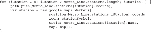
The
stationSymbol variable is a circle, one of the predefined symbols of the API, and it’s declared with the following statement:
The
path array is filled with the coordinates of each station and is used later as the path of the Polyline object that represents the metro line. After that, the code creates a Polyline object, the pLine local variable, which is the line’s path. The pLine variable is defined by the points already stored in the path array. The statement that creates the pLine variable is trivial, except for the icons property, which specifies the symbol of the train that represents the train on the line. This symbol is just a circle in this example, but you can design a nicer SVG graphic for the train’s symbol. Moreover, the symbol is placed initially at the beginning of the path (at 0 percent of its length) with the offset property of the icon object. Note that you can associate multiple symbols with the same line, and the related property is called icons. The icons property is an array of icon objects and in most cases, as in our example, it contains a single symbol. Listing 19-5 shows the statement that creates a Polyline object for the current metro line, based on the locations of the path array.Listing 19-5 Generating a polyline with a symbol at its end

Finally, the length of the path is calculated with the help of the
computeLength() method of Google’s geometry library:The argument to the
computeLength() method is an array of LatLng objects, which is exactly what the path array is: an array with the geo-coordinates of the line’s stations in their proper order. You just finished setting up the scene for the animation, and now you’re ready to explore the code of the animation function, which moves the trains.The Animation Function Instead of creating a function and passing its name as an argument to the
setInterval() function, the script uses an anonymous function definition in the setInterval() method’s code. It’s a very common approach among JavaScript developers, so you should see an example of a lengthy inline function definition. Listing 19-6 shows the call to the setInterval() function.Listing 19-6 The statements that animate the train along its path

The
distance variable is the actual distance covered so far and it’s increased by step meters at every cycle of the animation. The variable lineLength is calculated once outside the animation function because it doesn’t change during the animation. Because the animation function’s code is executed many times per second, it’s imperative that it’s optimized. The step variable is set to 12 meters and the animation cycle to 50 milliseconds with the following statements, which also appear outside the animation function:The train moves 12 meters every 50 milliseconds, or 12 × 20 = 240 meters per second, or 14,400 meters per minute. Assuming that the train moves at 45 kilometers per hour, which corresponds to 750 meters per minute, the animation progresses approximately 14,400/750 or approximately 20 times faster than the actual speed of the train.
Notice the statement that changes the sign of the direction variable:
The statement is executed only when the train’s location is at 0 percent or at 100 percent of its path. In other words, when the train reaches either one of its terminal stations, the
direction variable is toggled. This, in turn, toggles the direction of the train. When the train moves back, the currentPercent variable, which is the percentage of the length traveled so far, is calculated as usual. Then it’s adjusted by the following statement, should the direction variable indicate reverse movement:This statement says simply that the train’s location can be either 3 percent of the total length away from one end, or 97 percent of the same length away from the other end station. The first two
if statements in the code compare the percentage of the total length traveled so far to the values 0 and 1 (the two terminal stations). If the train is less than step meters away from either station, the program considers that the train has reached its destination. Because the trains will never reach the terminal stations exactly, the code toggles the direction of the train when the train is less than step meters away from the terminal station.Another statement that may not be obvious at first glance is the statement that calculates the current percentage of the route traveled:
The % operator is the modulus operator, which returns the remainder of the division. The distance
variable isn’t reset every time the train changes direction. Its value may become 64,500 meters after a while. The % operator in essence subtracts the number of integer lengths of the line and the result is the actual distance covered since the last direction change. The length of the blue line is 12,121.7 meters, and the operationyields the value 3,891.5. The train has traveled the entire line five times, and on its sixth route it has covered the first 3,891.5 meters. This is the value you must divide by
lineLength to figure out the percentage of the current route that has been covered already and place the symbol on the path accordingly. Note that changing the offset attribute of the symbol isn’t enough; you must also set the icon attribute of the polyline to force a redraw of the symbol:Open the
Paris Metro Simple.html page to examine the code and experiment with the various settings. Familiarize yourself with the program’s logic and then open the Paris Metro application, which animates all 14 metro lines. The following section points out the key differences between the two applications and how the animation technique applied to a single line is extended to handle all trains.Animating All Metro Lines
The
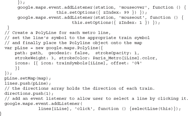
Paris Metro.html page is a web application that animates a train on every line of the Paris metro. The metro lines and their stations are stored in the Paris_Metro array, as discussed in the earlier section “The Application’s Data.” The script draws a different colored line on the map for every metro track and places the stations along each one of them. The stations are small filled circles with the same color as the corresponding line, and they’re placed on the map with the code shown in Listing 19-2. The animation function is a bit more complicated this time, as it must iterate through all the items in the lines array and animate a symbol on each one of them. It must also keep track of the lengths of all lines and reverse the direction of each train when it reaches the end of its line.To animate multiple trains, the script uses the animation function shown in Listing 19-7. It’s a lengthy listing printed here in its entirety to help you understand the animation logic.
Listing 19-7 The statements that animate multiple trains

The code that animates the train symbols is the same as before, but instead of the
lineLength variable (which was the length of the blue line), it uses the lineLengths array, which holds the lengths of the individual metro tracks. The symbols are animated in a loop that goes through each item in the lines array. In addition to the lineLengths array, this time the code uses the lines array. Where as in the simple version of the application you used the pLine object to represent the blue line, you now use the lines array to store a Polyline object for each metro line.Different trains change direction at different times because each line has a different length, and you need to store the direction of each train. Instead of the variable
direction, the script uses the directions array with a separate item for each metro line. The logic of the animation code is the same, only a bit lengthier.A very important aspect of an application that animates real-world entities is the elapsed time: how much actual time corresponds to the animation time. Let’s take a look at the statements that display the two times at the top of the page. To display the actual animation time, the code calculates the difference between the current time (variable
currentTime) and the time when the animation started (variable tStart) and formats it as hours:minutes:seconds. The calculation of the elapsed time involves the variable timeCount, which is increased by one every animation cycle. This time flies faster than real time by the specified scaling factor. The scaling factor of the animation time, in turn, depends on the animation cycle. If the animation cycle is 50, the animation time is scaled by a factor of 20 because the timeCount variable is increased 20 times per second. If the animation cycle is 1000, the scaling factor is 1, and the train appears to travel on the map at its real speed.Summary
This example concludes the first chapter on animating items on Google maps. I discussed in detail the animation of symbols along paths with data that has both a spatial and a temporal component. A moving object changes its position (the spatial component) with time (the temporal component). In the following chapter, I discuss another type of data: data that remains in place, but evolves with time. You’ve learned how to produce heatmaps; it’s now time to produce animated heatmaps that show how the intensity of the quantity they represent changes over time.
You will also see an application that animates an airplane over a geodesic path and the equivalent rhumb line on the map. You will actually “see” why geodesic paths are actually shorter than the equivalent rhumb lines, even though they appear to be longer on the map.
..................Content has been hidden....................
You can't read the all page of ebook, please click here login for view all page.