CHAPTER |
|
8 |
Feature Annotation: Drawing Shapes on Maps |
So far in the book, you have learned how to create map-driven web applications by embedding Google maps in your web pages. You also know how to place markers to identify points of interest on the map and how to write JavaScript functions to react to the basic map events. In this chapter, you learn about a more advanced, and very practical, feature of Google Maps: how to draw basic shapes on top of a map. Using shapes, you can mark features on the map, such as roads, borders of all types (besides administrative borders, which are displayed by default), even networks of lines that represent subway tracks, bus routes, gas pipes, electricity cables, any type of network. In some cases, it even makes sense to maintain the borders of states or countries as polygons. You can use these outlines to calculate the area of a state, or find out the state or county that was clicked, and so on. The borders shown on the map part of the image and you can't select countries or states on Google Maps.
The Google Maps API provides four objects that represent shapes: the
Polyline, Polygon, Rectangle, and Circle objects. Routes are represented by polylines, while property and administrative outlines are represented by polygons.NOTE The word “shapes” refers to closed geometric entities, which are represented on Google Maps as polygons. Strictly speaking, a shape is a polygon. In the context of this book, I use the word “shape” to refer to polylines, rectangles, polygons, and circles. And sometimes I use the term “line” to refer to polylines. Also, the terms “polyline,” “polygon,” and “circle” in the text refer to the usual geometric entities, while the terms “Polyline,” “Polygon,” and “Circle” are the names of the objects that represent the corresponding entities on the map.
Polylines
A polyline is a collection of connected line segments, defined by a series of locations. The locations form the polyline’s path, which is an array of
LatLng objects. These locations are the line’s breakpoints and are known as vertices. Figure 8-1 shows a polyline that corresponds to one of the lines of the Los Angeles metro system, the Golden Line. The figure was generated by the LA Golden Metro Line.html page, included with this chapter’s material. The stations are marked with RichLabel controls, as you recall from the preceding chapter.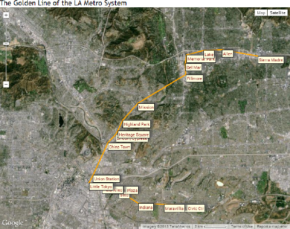
Figure 8-1 The polyline on the map is based on a path formed by the locations of the stations of the Golden Line of the Los Angeles Metro System.
The polyline that represents the metro track is defined by the locations of the stations along the metro line and the tracks between stations are straight line segments. This is an oversimplification, of course, because rail tracks don’t change direction abruptly. If you can specify more points along the line’s path, you’ll be able to display a smoother line on the map that follows more closely the path of the metro line and has the appearance of a smooth curve. Even so, when users zoom deeply, they will be able to see the breaks in the line.
When you trace a map feature such as a freeway, a river, or a rail track with too many points, the resulting polyline can approximate any shape, including smooth curves. Figure 8-2 (see page 166) shows the outline of Italy. The shape is actually a polygon (a closed polyline), but it’s still defined by a path. Italy’s outline is made up of 639 vertices and up to a reasonable zoom factor it approximates the country’s borders nicely.
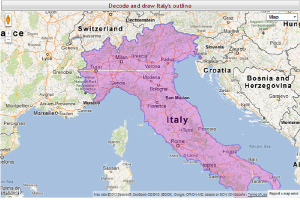
Figure 8-2 A polygon encompassing Italy
The data was generated with a Windows application, the Map Tracing application, which is discussed in Chapter 9. The Map Tracing application allows users to trace any map feature interactively and keeps track of the locations specified by the user on the map.
Polyline Construction
To place a polyline on the map, you must create a
Polyline object and place it on the map by calling its setMap() method. The constructor of the Polyline object expects an array of LatLng objects that define the polyline’s path. This array must be passed to the constructor with the path attribute. Here’s a short segment of the definition of the metro line’s path:
The first two coordinates correspond to the Atlantic and East LA Civic Center stations of the Golden Line; open the sample page to see the entire track. The following statement creates a very basic
Polyline object, which will be rendered on the map with the default color and default width:The
path attribute is the only mandatory attribute of the Polyline object. To specify any of the optional attributes, add more items to the array following the constructor. The other two basic attributes of the Polyline’s constructor are the line’s width, which is specified in pixels, and its color. Because the polyline has a color, it can also have an opacity value.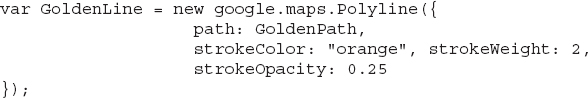
To actually place the
GoldenLine object on the map, you must call its setMap() method, passing the name of a Map object as an argument:You can change any of the properties of the line in your code by calling the
Polyline object’s setOptions() method, which accepts as an argument an array of key-value pairs: The keys are property names and the values are the property values. The following statement changes the color and width of the line on the map:You can also change the path of a polyline with the
setPath() method, which accepts as an argument another path.Polygons
Polygons are very similar to polylines: In effect, polygons are closed polylines. They’re also specified with an array of locations (or vertices) with the
path attribute, and they have a strokecolor and a strokeWeight attribute. In addition, you can specify the polygon’s fillColor attribute. Note that polygons are always closed and you don’t have to repeat the initial point to close the shape because the end point will be connected to the initial point automatically. In effect, you can use the path of a polyline to create a polygon with the exact same shape.You can change any attribute of a polygon at will by calling the
setOptions() method and passing as argument an array with the attributes you want to change and their new values, similar to the array passed to its constructor.To prepare a nontrivial shape, the outline of Italy was traced with the Map Tracing application, which is discussed in detail in Chapter 9. The path of the outline consists of 639
LatLng objects, and the polygon of Figure 8-2 was based on this path. The polygon encloses the continental part of Italy. As you probably know, Italy encompasses two large islands, as well as many smaller ones. Additional shapes can be defined with additional paths, as you will see in the section “Polygon Islands” later in this chapter. The polygon looks quite reasonable at a moderate zoom level. As you increase the zoom level, the differences between the actual borders on the map and the polygon’s shape become noticeable.Polygons with Holes
A polygon may contain a hole, like the one shown in Figure 8-3. To define the shape shown in the figure, you need two polygons: one for the outer shape and another one for the hole. Indeed, the path of a polygon with holes is an array of paths. In JavaScript terms, this is an array of arrays. The first path in the array is the path of the outer polygon and the remaining paths correspond to holes, as long as these paths are fully contained within the outer polygon. Figure 8-3 shows the state of Utah with a hole that corresponds to Utah Lake. If the shape of the lake is hard to see on the printed page, please open the
Polygons.hml page.
Figure 8-3 The outer polygon is the state of Utah and Utah Lake is rendered as a hole within the state’s polygon.
The
Polygon object provides two methods for specifying its shape: setPath()and setPaths(). The difference between the two methods is that setPaths() allows you to specify multiple paths for the polygon. The first shape is the basic polygon and the remaining ones represent holes in the outer shape. The state of Utah with a hole that corresponds to Utah Lake was generated with the drawPolygon() function, which accepts as an argument the path of the shape to draw: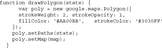
The
state argument is either a path (an array of vertices) or an array or paths, each path being an array of vertices. The statements shown in Listing 8-1 create the path for the state of Utah, and call the drawPolygon() function with the path of Utah as argument. The path of Utah is made up of two paths. The first is the outline of the state and the other one is the outline of Utah Lake, as shown in the following listing. The resulting shape is commonly referred to as “donut-shaped.”Listing 8-1 Constructing a “donut”-shaped path
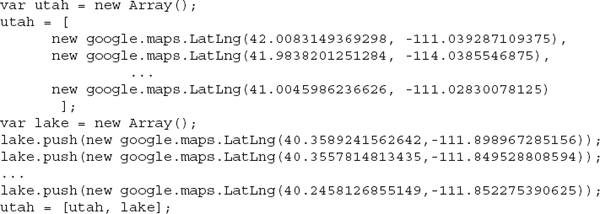
Most of the locations were skipped in the preceding listing, as the number of vertices or the complexity of the shape won’t make any difference. Note the different methods used to specify the two arrays: the
utah array is populated in its initializer, while the lake array was populated by pushing one element at a time. Open the file Polygons.html, which draws the outlines of three states on the map. One of the states is Utah, which includes a polygon that delimits Utah Lake. The other two polygons correspond to Nevada and Wyoming, whose borders are made up of large straight lines.Polygon Islands
Figure 8-4, on the other hand, shows the outline of Los Angeles County, which is made up of three polygons: one for the continental part of the county and two more for the islands outside Los Angeles. Because the two islands are totally outside the polygon that corresponds to Los Angeles County, they’re rendered on the map as regular polygons.

Figure 8-4 The county of Los Angeles includes the Santa Catalina and San Clemente islands, in addition to the continental part of the country.
If you open the
Islands Polygons.html file, you will see that the script creates a single Polygon object with a path that contains three arrays. Listing 8-2 shows just the basic statements of the script.Listing 8-2 Creating a path with “islands”

The ellipses indicate missing definitions of
LatLng objects. The three individual paths are combined into an array of paths, the LosAngelesPath variable, which is then passed to the Polygon object’s setPaths() method. Note that you must use the setPaths() method, even if you're passing a single array as an argument, because the argument is an array of arrays.Displaying a Crosshair on the Map
Another interesting use of the line drawing feature of the API is the implementation of a crosshair at the center of the map. Typical mapping applications allow users to precisely locate the desired features on the map. You can program the map’s
click event and expect that users will identify a location with the mouse and click on it. This approach is neither precise nor user friendly. A better approach is to display a crosshair cursor at the center of the map, like the one shown in Figure 8-5, and allow users to scroll the map until they bring the location they’re interested in exactly under the crosshair.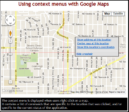
Figure 8-5 The
Context Menu.html web page allows users to show and hide a crosshair cursor on the map.The crosshair is a pair of vertical lines that meet at the center of the map. To draw them, you need to know the horizontal and vertical extents of the map’s viewport and then draw two lines through the middle of each axis and extend from the minimum to the maximum latitude or longitude. The drawing of the lines takes a few statements, but it’s straightforward; you will use the map’s
getBounds() method to retrieve the horizontal and vertical extents of the current viewport.However, you must redraw the two lines every time the user drags the map around, as well as when the user zooms out. The code that draws the two lines of the crosshair on the map must be executed from within the map’s
bounds_changed event. Otherwise, the crosshair will scroll with the map because it was drawn at a specific location on the map. Moreover, users may not wish to keep the crosshair visible at all times, so you must give them the option to show or hide the crosshair. In Chapter 5, you saw how to add to the context menu a command that shows/hides the crosshair. Now that you know how to draw lines on the map, let’s look at the statements that actually draw the crosshair of the Context Menu.html sample page of Chapter 5.First, you must declare three variables: two variables that represent the two lines and the
crosshair variable that indicates the visibility of the crosshair. Set the crosshair variable to true or false to control whether the crosshair will be displayed initially.
The
drawCrosshair() function does all the work. It extracts the coordinates of the minimum and maximum latitude and longitude values, calculates the coordinates of the endpoints of the two lines, and then draws them on top of the map. The code of the drawCrosshair() function is shown in Listing 8-3, which is a bit condensed to fit on the printed page.Listing 8-3 Drawing the two lines that form a crosshair cursor at the map’s center

The variables
centerHLine and centerVLine are two Polyline objects that represent the two lines that make up the crosshair. The horizontal line’s latitude is the latitude of the map’s center point, and it extends from the minimum to the maximum visible longitude. Similarly, the vertical line’s longitude is the longitude of the center point, and it extends from minimum to the maximum visible latitude. The script relies on the crosshair variable, declared at the script’s level, which indicates whether the crosshair cursor is visible at the time. If the cursor is not currently visible, the script draws two perpendicular lines that meet at the center of the map. If the crosshair is visible, then the script removes the cursor from the map by setting the map attribute of the centerHLine and centerVLine variables to null.Rectangles
Rectangles are, in effect, polygons with four vertices, but they’re defined without a path. Instead, they’re based on a
LatLngBounds object, which describes both the location and size of the rectangle. Other than that, they have the same properties as polygons. In fact, you can create rectangular polygons and ignore the Rectangle object. Use the StrokeColor and FillColor to specify their appearance, the StrokeOpacity and FillOpacity properties to set the rectangle’s opacity, and the StrokeWeight to set the width of the rectangle’s outline.To create a new
Rectangle object, use a constructor like the following:
Only the
bounds property is mandatory; all other properties are optional. The LatLngBounds object’s constructor accepts two arguments, which are the coordinates of the lower-right (south-west) and upper-left (north-east) corners of the rectangle. While polylines and polygons are used extensively in mapping applications, there aren’t many features that can be approximated by rectangles and circles. These two shapes are too perfect for the shapes you usually mark on the map.Circles
Circles are defined by a center point and a radius. The center is a
LatLng object as usual (a location on the map), and the radius is specified always in meters. Here’s the constructor of the Circle object:
The circle is located at the center of Liberty Island in New York and its radius is 1 kilometer. You can set the circle’s center and radius from within your code at any time by calling the
setOptions() method as usual, or the setCenter() and setRadius() methods, passing the appropriate value as argument. As far as events go, you can detect the usual mouse on the circle as well as the center_changed and radius_changed events, which aren’t very common in coding mapping applications. You can fill the circle with a solid color to create a disk with the strokeColor and strokeOpacity properties.Unlike polygons, you can’t place holes in circles or use circular holes in polygons. However, you can create a polygon that approximates a circle with a function that generates points along the circle’s circumference and then uses these points as a path. If you generate 100 or 200 points along the circumference, the polygon will be a good approximation of the corresponding circle. This approximation isn’t recommended because the more points you add to your polygon to better approximate the circle, the slower your script will get. On the other hand, it’s the only way to create circles with holes, or circular holes, in another polygon.
Listing 8-4 show the
drawGeodesicCircle() function, which approximates a circle by creating a polygon with 500 vertices, all on the circumference of the underlying circle. The function performs simple trigonometric calculations. Okay, they aren’t simple because the circle is drawn on a sphere, but it’s not much different from calculating points along the circumference of a circle on a flat surface. Most readers who need this function will simply paste it in their script, so I won’t get into advanced trigonometric topics here.Listing 8-4 Approximating a circle with a polygon
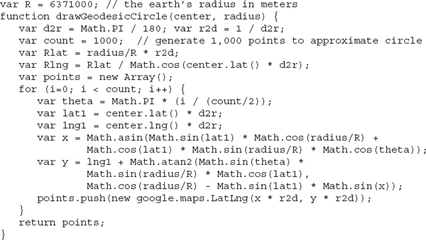
The
drawGeodesicCircle() function accepts two arguments, the circle’s center and its radius, and returns an array of LatLng objects, the points array, which you can use to draw a polygon that approximates the equivalent circle. You may have noticed that the name of the function is drawGeodesicCircle() and not drawCircle(). A geodesic circle is a perfect circle on the sphere, not on the flat map. At smaller scales, the two circles are identical because small sections of the earth’s surface are practically flat. At large scales, when the circle’s radius exceeds 1,000 kilometers, for example, the perfect circle on the sphere is not nearly as perfect when projected onto the flat map. The topic of geodesics, along with the distortion introduced by projecting large earth features on a flat map, is discussed in detail in Chapter 10. In the same chapter, you will find more interesting examples of circles drawn on a Google map.Fixed-Size Circles
There’s no option to specify the
Circle object’s radius in pixels; this will cause you problems if you’re trying to use a circle as a marker on the map. Because the circle’s radius is defined in meters, its actual size will follow the zoom level. If you zoom out far enough, the circle will practically disappear, and if you zoom too deeply, the circle may fill the entire map.What if you want to display a circle that retains its size at all zoom levels? The solution is to specify the radius not in absolute units, but as a percentage of the map’s width. Moreover, you must redraw the circle with its new radius every time the user changes the zoom level. In Figure 8-6, you see a web page created to demonstrate animation techniques for Chapter 20. When the user clicks somewhere on the map, a “vanishing” circle is displayed for a few moments at the location of the click. The circle’s opacity goes from 1 to 0 in a second or so, and the circle disappears. This simple animation effect, however, is a very effective way of highlighting the point that was clicked.
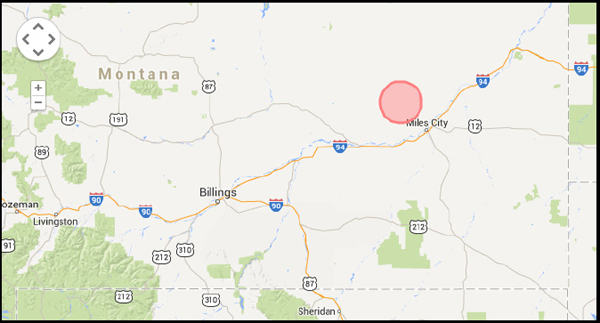
Figure 8-6 The
Highlight Points.html page uses animated circles to highlight locations on the map.You will see the complete code of this technique in Chapter 21, but let me show here quickly the code that calculates the radius of the circle. When the user clicks on the map, the following statement calculates the horizontal extent of the map in degrees:
To convert this value to meters, you multiply it by 111,320 because each degree corresponds to 113.32 kilometers on the surface of the earth (near the equator, of course). Then, you can set the circle’s radius to 2 percent or 5 percent of the viewport’s width. The following statement sets the radius to 2 percent of the map’s viewport:
The actual size of the circle will be different at different latitude values; this technique draws a consistently small disc that may not have the exact same size at all locations, but it changes size as you zoom in or out so that it appears to have a more or less constant size at any zoom level.
Another approach to drawing circles the same size at all zoom levels it to use icons instead of circles. In the section “Placing Symbols Along Polylines” later in this chapter, you will see how to use the built-in symbol of a filled circle to identify a feature on the map.
Storing Paths in MVCArrays
The
path property of the polylines and polygons is an array of geo-locations; you can manipulate the shape’s outline by manipulating the elements of the path. However, changing an element’s value won’t have an immediate effect on the shape that has been rendered on the map. You must create a new object based on the revised path and place it on the map, in place of the previous version of the same shape.Google provides a special object, the
MVCArray, which can be bound to another entity. As you recall from Chapter 4, MVC stands for Model-View-Controller. It’s a design pattern that allows the same data to be presented in different manners. As soon as the data is updated, the view of the data is also updated. The MVCArray object can be bound to a path or other object and update the object it’s linked to. If you use a MVCArray to store the shape’s path and then assign this object to the shape’s path property, the path property will remain bound to the MVCArray. This means that every time you change an element in the MVCArray, or add a new vertex to the path, the shape will be updated automatically. MVCArrays are extremely useful in programming with the Google Maps API because they allow you to focus in your code, and not the plumb work required to keep the map up-to-date. If you stored the vertices of a path to a regular array and then assigned this array to the path property of a polygon, the polygon would assume the shape of the path the moment of the assignment. After that, you could change the array without affecting the shape; you would have to reassign the array to the path property to change the polygon’s shape.Figure 8-7 shows a Google map with a polyline on it. The vertices of the polyline are identified by markers and you can edit the shape by moving the markers around with the mouse. Figure 8-7 was created by the
Editable PolyLine.html application; the script that drives the functionality of this page is discussed in the following section.
Figure 8-7 Editing a line on the map by dragging the markers on its vertices with the mouse
The core of the script is an
MVCArray object with the path’s vertices. This array is used as the shape’s path so that when a vertex is moved and the code updates the selected vertex’s location, the shape changes instantly.An Editable Polyline
Specifying a polyline and placing it on the map is straightforward, and you can create complex overlays on top of the map using the
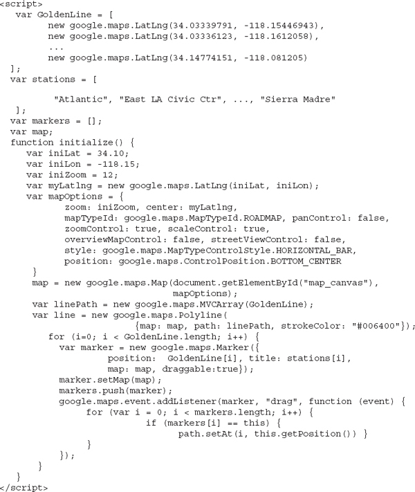
Polyline and Polygon objects. What if you want to create a new shape by tracing a feature on the map, such as a train track, a delivery route, a network of cables, and so on? Wouldn’t it be useful to be able to edit the polyline right on the map? Indeed, this is one of the most basic features of a GIS system, and you’re going to build an application for tracing maps in Chapter 9. In this chapter, you will find all the information you need for designing editable polylines and polygons. The Editable PolyLine.html page shown in Figure 8-7 demonstrates a technique for editing a polyline interactively. Each vertex of the polyline is identified by a marker and users can edit the polyline by dragging the markers with the mouse. This isn’t exactly an editable polyline because this technique doesn’t allow users to delete vertices or insert new ones, but it’s the first step in designing truly editable polylines.The polyline shown in the figure represents a metro line, and its vertices are the stations along the line (which happens to be the Golden line of the Los Angeles Metro). The data is stored in two arrays in the script: the first array,
GoldenLine, contains the coordinates of the metro stations, which are also the polyline’s vertices, and the other one, the stations array, contains the names of the stations. Here are the constructors of the two arrays:
The script starts by creating a variable for storing the polyline’s vertices, the
linePath variable. The linePath variable holds the coordinates that define the polyline based on the GoldenLine array. However, the script generates an MVCArray object based on the GoldenLine array. It does so by passing the GoldenLine array as an argument to the constructor of an MVCArray object. The linePath array is then used to specify the polyline’s path in the Polyline object’s constructor. The following two statements place on the map a polyline that represents the Golden line of the Los Angeles Metro:The script iterates the
GoldenLine array and generates a marker for each station. The statement that generates the markers is straightforward; just note that the draggable property is set to true so that the users of the application can edit the polyline by dragging around the markers that correspond to the polyline’s vertices:
Note that each new marker is added to the
markers array so that the script can access the markers later. If you don't store the individual markers to an array, you won't be able to manipulate them after they have been placed on the map.So far, you have displayed a polyline on the map and placed a marker at each vertex. The markers are draggable, but they can’t be used yet to edit the shape of the polyline. For this to happen, you must change the location of the corresponding vertex in the path as the user moves the marker. This action must clearly take place in each marker’s
drag event listener. In the listener’s code, you must find out the index of the marker being dragged in the markers array and use this index to access the corresponding vertex in the path to change its coordinates. Here’s the statement that adds the appropriate listener to each marker’s drag event: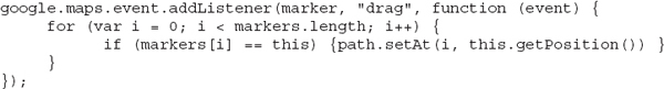
The loop iterates through the
markers array and compares each marker to the marker that fired the event (identified by the keyword this). When the marker being dragged is located, the code changes the value of the corresponding item in the path array and sets it to the marker’s current location, which is given by the expression this.getPosition(). The code is short and simple, but thanks to the ability of the elements of the MVCArray object to remain bound to the polyline’s vertices, the polyline’s shape is changed as soon as you change the location of any vertex. Listing 8-5 shows the complete script of the Editable PolyLine.html page (the ellipses in the two array initializers stand for additional elements omitted from the listing).Listing 8-5 Displaying a polyline with markers at its vertices on the map
Open the
Editable Polyline.html page and test-drive it. You have a truly interactive map that allows you to position markers very precisely with the mouse. To create an editable polygon, you need only change the definition of the Polyline object to a Polygon object. The polygon you specify with the same path will remain closed at all times as you edit its path, without any additional code.As soon as an element of the
path array changes, the polygon is redrawn on the map and its new shape is dictated by the current locations of its path’s vertices. The short application you created in this section is the beginning of an interactive map drawing application. This is the topic of the next chapter, where you will implement an application that allows users to edit shapes interactively on top of the map.Placing Symbols Along Polylines
An interesting feature added to version 3.0 of the Google Maps API is the capability to place symbols along polylines, as shown in Figure 8-8. The highway was drawn with the
Highway 5.html page, included in this chapter’s support material.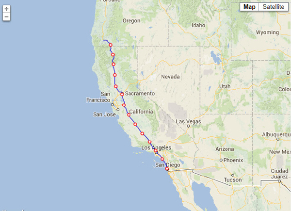
Figure 8-8 Repeating a symbol along a polyline path. The line shown here corresponds to the US 5 highway in California.
The symbols may be placed at fixed positions, or they can be repeated along the polyline, and they usually indicate direction. If you make the underlying polyline invisible and place the symbols close to one another, then the symbols are no longer “decorations”; they become the line. This is how you can create dotted and dashed lines on top of a map.
Consider the following path definition:

These are the first few vertices of a path that correspond to a large segment of the US 5 Highway from San Diego to Portland. It’s a plain polyline that was traced manually with the Map Traces application, which will be discussed in the following chapter.
Let’s add a few marks along the highway. First, you must create a new symbol with a statement like the following:

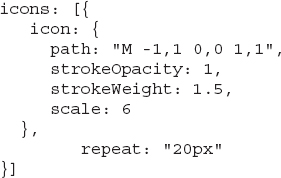
The symbol is defined as an array of property values. The symbol’s shape, specified with the
path property, is one of the predefined symbols that come with the API, and it’s a circle. The predefined symbols are members of the google.maps.SymbolPath enumeration, which includes the following: CIRCLE, BACKWARD_CLOSED_ARROW, FORWARD_CLOSED_ARROW, BACKWARD_OPEN_ARROW, and FORWARD_OPEN_ARROW. In addition to the API’s predefined symbols, you can create your own symbols using the SVG (Scalable Vector Graphics) notation, which is discussed briefly in Chapter 20 and Appendix A. The symbol created with the preceding statements is a white circle with a medium-width red outline. The scale attribute is very important: It’s the scaling factor of the symbol in pixels. The default size of the symbol (when scale is 1) is the same as the polyline’s stroke width. Because their sizes are specified in pixels, symbols are not affected by the zoom level: They have the same size at all zoom levels.To place instances of the selected symbol along the path of the polyline, you must set the
Polyline object’s icons property. This property is an array of symbols, and it usually contains a single item. In addition to the symbol, you must also specify one of the offset or repeat properties. The offset property is the distance from the beginning of the line, where the symbol will appear; it can be expressed either in pixels or as a percentage. This property’s default value is “100%” (it’s a string). The repeat property is used when you want to repeat the symbol along the line’s path; its value is the distance between successive symbols on the line and it can be expressed either in pixels or a percentage. The following is a typical icons property definition: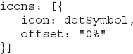
If you use this definition in a
Polyline object’s constructor, the specified symbol will appear at the beginning of the line. A more interesting example is the following, which repeats the symbol every 25 pixels along the path, as shown in Figure 8-8.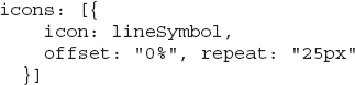
The complete statement that produced the path shown in Figure 8-8 follows. The array
US5 holds the vertices of the path, and the icons property determines the symbol and how it will be repeated along the path. The symbol is a circle icon, identified by the dotSymbol variable created earlier, and it’s repeated every 25 pixels. All these settings are combined in the constructor of the US5Route object, which is a Polyline object.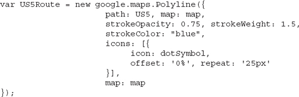
The most important aspect of symbols is that they can be animated. In Chapter 20, you will see applications that animate a symbol along a line to simulate an object, such as a train or airplane, traveling between any two locations.
Another interesting application of symbols is to create dashed and dotted lines. To create dashed lines, you must use the SVG notation, which is discussed in detail in Appendix A. In the same appendix, you will find examples of different line types. There’s also a short demo page by Google that demonstrates various types of dotted lines. The page animates the symbols too, but you can ignore the animation for the time being. Just copy the SVG definitions of the various line shapes and re-use them in your code. The URL of this page is http://gmaps-samples-v3.googlecode.com/svn/trunk/symbols/polyline-symbols.html.
The definition of the chevron symbol on this page, for example, is as follows:
The highway was traced with over 1,000 vertices, and you can see that it doesn’t quite follow the freeway’s path when you zoom in too closely. Figure 8-9 shows two details of the same highway. Note that the symbols do not get closer or further apart as you zoom in and out because the icon’s
repeat attribute is specified in pixels, not as a percentage. The distance between consecutive symbols in Figure 8-9 is the same, even though the second map of Figure 8-9 covers a tiny segment of the highway.
Figure 8-9 When the symbols are placed apart by a number of pixels, their density is the same regardless of the zoom factor.
Handling Large Paths
In this chapter’s examples, all the coordinates required to generate paths were embedded in the corresponding scripts. This is convenient for sample applications, but it’s not very practical for real-world applications. The main drawback with this approach is the size of the script. There are two techniques for transferring the definitions of large paths to the client, both of which are discussed later in this book. Here's an overview of these two techniques.
The first technique uses compressed paths. Google provides the tools necessary to encode long paths as text in a compressed format. This format isn’t readable; it looks like this:
Just a segment of an encoded path is shown here. It’s a binary value encoded as text using the Base64 format, but you need not understand anything about Base64 encoded values. You can encode your paths into similar strings, transmit the strings to the client, and then decode the path in your script to generate the original path. The topic of encoding and decoding paths is discussed in Chapter 10 and in the file “The Encoding Library.pdf” included in this chapter’s support material. The advantage of embedding the data into the script, using either encoded format or the plain-text format, is that after the page has been loaded, the data is instantly available to the script and no more trips to the server are required.
The second approach is to request the necessary paths on demand from the web server where your application is hosted. The script contains just code (and a few data items to initialize the map, perhaps) and is short. The data that defines the shapes on the map is fetched as needed from the server. On the server, you may store the data in files, or write a web service that retrieves the requested data from a database (or a local XML file, or even another remote web service) and returns it to the client script in any format you see fit. XML is a format for data exchange discussed in Chapter 10, along with an XML variation specific to geographic data known as KML (Keyhole Markup Language). XML is the universal standard for data exchange between systems today, and it’s also easy to understand.
You can also push the data to the client in JSON format (the format used to describe custom objects in JavaScript, as you recall from Chapter 4). The web service may also accept arguments that determine specific datasets. For example, you can write a web service that returns the path of a metro line and expects the number or the name of the metro line as an argument. The advantage of requesting data through a web service is that the client application gets up-to-date data every time it calls the web service, and it retrieves just the data needed at the time. The topic of accessing remote web services from within a script is discussed in detail in Chapter 15.
Summary
In this chapter, you learned how to place simple drawings on a map. The shapes you read about in this chapter are all the shapes supported by Google Maps, and they’re the same shapes you would use with most GIS systems.
The three geometric entities you can place on a map are lines, polygons, and circles. Lines are one-dimensional objects and have a length. Polygons are two dimensional objects and have a perimeter (which is basically their length) and area. In Chapter 10, you will learn how to calculate these attributes. It should be mentioned here that these shapes are “plastered” on a sphere and the calculation of length and area are not trivial. Fortunately, the geometry library of the API provides methods for these calculations. The geometry library of the Google Maps API is covered in detail in Chapter 10, where you will also learn how to compress paths by encoding their vertices. The geometry library also exposes methods for calculating polyline lengths and polygon areas.
You also saw the basics of editing simple shapes interactively on top of the map. The following chapter elaborates on this technique, and then you can proceed to build a highly interactive GIS application.
..................Content has been hidden....................
You can't read the all page of ebook, please click here login for view all page.