CHAPTER 2

Shortwave and Allwave Listening

The frequency range from 3 MHz to 30 MHz (wavelengths of 100 meters to 10 meters) is sometimes called the shortwave band. You can build or buy a shortwave radio receiver, install an outdoor wire antenna, and listen to signals from all around the world in an activity called shortwave listening (SWL). If you extend the receiving range below 3 MHz down to the lowest frequencies you can get a radio to bring in, and if you can also extend the range above 30 MHz up to the highest frequencies you can manage, you can think of the hobby as allwave listening (AWL). In the United States, you don’t need any sort of license to engage in radio listening at any frequency. In some countries, however, you will have to get a license to receive radio signals (believe it or not). If you don’t live in the United States, check with your government authorities before you get involved with SWL or AWL.

 

How I Got into SWL

My SWL experience dates back to elementary school in the 1960s, when my dad bought me a radio project kit for my birthday. I was in the third grade, and even as I write this chapter, I have a note that I wrote to myself that year (1963), stating that I intended to become an Amateur Radio operator by the time I turned 10 years old. (Actually it took me until the sixth grade, at age 12.) I don’t know how I would have heard about ham radio, were it not for SWL in those days of stuffing pieces of wire into spring contacts on a circuit board with capacitors, coils, resistors, and a 1T4 vacuum tube about the size of my thumb that ran off of a 45-volt battery and a 1.5-volt flashlight cell.

The first few projects involved simple broadcast receivers, such as a “crystal set” that worked without a battery, progressing to a battery-powered radio with an audio amplifier after the detector, and then adding other components to increase the selectivity and sensitivity. I recall hearing WLS in Chicago on that radio at night, and marveling at the vast distances over which radio waves could travel over free space to reach me, in my bedroom with that earphone clamped against my head in Rochester, Minnesota! My fascination with radio began back then.

Later projects with that kit included substitution of a different antenna coil, one that looked smaller than the original. It supposedly provided shortwave reception, but it didn’t bring in much of anything until I got to the project called the “Regenerative Grid Leak Detector with Pentode Amplifier.” Then I heard signals from all over the world: strange languages, bizarre buzzing and swishing and whining noises, and a time-standard station that claimed to come out of some observatory in Canada. I could tune through all of this cool stuff with a variable capacitor no larger than a golf ball.

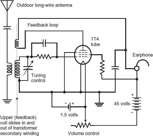
FIGURE 2-1 Generic diagram of the circuit for my first shortwave radio project, according to my best recollection. I don’t remember the component values.

My dad introduced me to other hobbies aside from radio; he was the sort of father every kid should have, encouraging me to find and chase my own interests. He never told me where to “sail,” but he made sure that I had good “boats.” He bought me a small refracting telescope to complement his own big Newtonian reflector; I got a pretty good microscope one year too. But it was that radio kit that pointed me toward my final career: to work for companies that dealt with Amateur Radio issues and equipment, and later to write about hobby electronics in books like the one you’re reading right now.

In the fifth grade, I got a more sophisticated, commercially manufactured shortwave radio receiver, the Hallicrafters model SX-130. I recall its appearance in every detail. It used a single-conversion, superhet design of the sort shown back in Chap. 1 (Fig. 1-16), along with extra audio amplifiers so that the sound could drive a loudspeaker. Like nearly all shortwave radios in the mid-1960s, the SX-130 worked with vacuum tubes. It covered frequencies from the bottom of the standard AM broadcast band at 535 kHz up to the top of that band at 1.605 MHz, had a little gap where it didn’t receive anything, and then allowed reception over a continuous range of frequencies from 1.725 MHz to 31.500 MHz.

The SX-130, like most state-of-the-art shortwave radios of its day, employed two tuning dials, one called main tuning and the other called bandspread. The bandspread scale had a “slide-rule” geometry with multiple scales, but it gave accurate readings only when the main tuning dial was set at specific points. The SX-130 did not have an internal calibrator, so I had to guess at the exact frequency to which the radio was set. I learned how to “tweak” the main tuning dial to get reasonable bandspread scale accuracy by taking advantage of the National Bureau of Standards (now called the National Institute of Standards and Technology) time-and-frequency standard broadcasts. The station had the call sign WWV back then, as it does today. I would set the bandspread to a known WWV frequency and then carefully manipulate the main tuning dial to make the signal come in just right.

I sat for hours in front of that radio, fascinated, listening to the beeps and buzzes and tones and ticks that WWV produced (one of which I recognized as a sound effect in an episode of the original Star Trek television series). I learned that the Canadian station I had heard with the regenerative radio receiver kit had the call sign CHU, transmitting at 7.335 MHz. I discovered cryptic conversations taking place among individuals in frequency bands around 3.5 MHz, 7 MHz, and 14 MHz. I heard Morse code and other unidentifiable signals that sounded as if they could just as well have come from extraterrestrial civilizations. Before very long, I realized that these emissions came from hobby radio operators using transmitters in their own homes: radio hams!

When I entered the sixth grade in the fall of 1965, I started taking a ham radio class in my hometown, offered by the Rochester (Minnesota) Amateur Radio Club. In March of 1966, I got my Novice Class License, which, back in that day, offered severely restricted privileges. I had to learn to send and receive Morse code at five words per minute. I actually had to write down what I heard on the spot, for a solid continuous minute or more, without a single mistake. I had to send a solid minute of code error-free too, at that same five words per minute. But I finished the course somehow, and got my Novice Class License. My exuberance knew no bounds when I made my first contact on 7.185 MHz with a radio ham in Zeeland, Michigan, using Morse code that I pounded out with a simple telegraph key. I still have that key in my “ham shack” today, although I don’t use it anymore.

 

Shortwave Broadcast Bands

International shortwave broadcasting takes place in several bands covering well-defined frequency intervals, with the lowest frequency (longest wavelength) at 2.300 MHz. Table 2-1 shows the shortwave broadcast bands designated at the World Radio Conference in 1997. The complete span of frequencies covers more than an order of magnitude (factor of 10), that is, the top frequency on 11 meters is a little more than 10 times the lowest frequency on 120 meters. Let’s look at how these bands behave, so you’ll have an idea of what to expect when you tune your radio to them.

TABLE 2-1 International Shortwave Radio Broadcast Bands

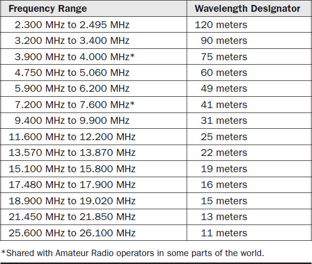
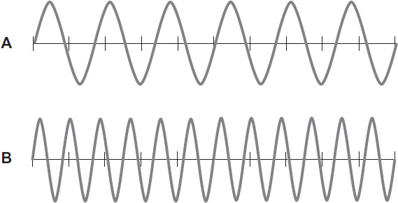
FIGURE 2-2 In free space, wavelength varies inversely with frequency. In this example, the wave at A has half the frequency of the wave at B. A complete wave cycle at A, therefore, measures twice the length of a complete wave cycle at B.

120 Meters

Radio-wave propagation at 2.300 MHz resembles that at the upper end of the standard AM broadcast band. The effective range at night greatly exceeds the range during the day because when the sun is above the horizon, the ionosphere’s D layer absorbs radio waves at this frequency before they can reach the higher layers. At night, the D layer disappears, and you can expect worldwide reception from stations that use high RF output power levels (several kilowatts or more). Conditions peak during the winter months, especially at the higher latitudes where thunderstorms don’t occur often at that time of the year. Thunderstorms produce sferics (sometimes called “static”), a form of radio noise that can impede or ruin signal reception. In addition, during the fall and winter, more of your hemisphere lies in darkness than is the case in the spring and summer, so you can enjoy the advantages of nighttime conditions for a greater portion of the day.

90 Meters

In the range of frequencies from 3.200 MHz to 3.400 MHz, signals propagate better at night than during the day, just as they do on the 120-meter band and the standard AM broadcast band. You might notice improved reception here, compared with 120 meters, from transmitting stations that use modest output power levels. If you have done much operating on the ham radio 80-meter and 75-meter bands (3.500 MHz to 4.000 MHz), you’ll already have a good idea of how things work on the 90-meter shortwave broadcast band, and vice versa. As with 120 meters, conditions tend to peak in the winter (for the same reasons).

75 Meters

The shortwave band at 3.900 MHz to 4.000 MHz lies within the American ham radio 75-meter voice band, so ham radio operators must share the spectrum with these stations. Because shortwave broadcasting transmitters generally use more power than ham radios do, Amateur Radio operators sometimes find communication difficult in the top 100 kHz of their 75-meter band. When you listen to signals in this band, you can tell the difference between ham radio stations and shortwave broadcast stations. Ham radio operators use SSB emission, requiring a receiver with a local internal oscillator, but broadcast stations use AM emission, and you can bring them in with a simple envelope detector. Excellent worldwide shortwave reception can be had at night on this band, especially in the winter at latitudes far from the equator, because there’s not much thunderstorm static and the darkness hours last a long time.

60 Meters

In the range 4.750 MHz to 5.060 MHz, you’ll hear shortwave broadcasts on the so-called 60-meter band. As with 75 meters, worldwide communications and reception take place at night. During the daylight hours, signals can travel a few hundred kilometers, significantly farther than they do on the lower frequencies. As with the lower-frequency bands, conditions peak in the winter when thunderstorms occur less often and the nights last longer. Good conditions can sometimes exist on this band during the spring, summer, and fall months, especially in places such as the West Coast of the United States where thunderstorms rarely occur at any time of year. Ham radio operators have a small frequency allocation near this band. If you hear SSB or CW signals in this part of the radio spectrum, they’re probably coming from ham radio stations, especially if they’re around 5.3 MHz to 5.4 MHz.

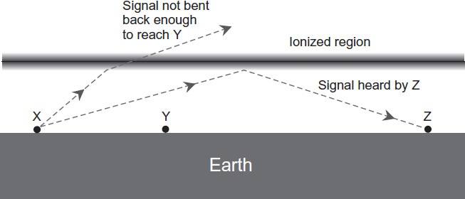
FIGURE 2-3 Station X transmits a signal that reaches the ionosphere, which bends back the waves enough to reach station Z but not enough to reach station Y. Station Y, therefore, lies within the skip zone with respect to station X at the frequency of interest.

49 Meters

In the 49-meter band (5.900 MHz to 6.200 MHz), conditions are much the same as they are at 60 meters, although you’ll occasionally see a skip zone form. Also, atmospheric noise tends to present less of a problem, so you can get good reception during the spring, summer, and fall as well as in the winter. Once in a while, you’ll hear stations as far away as 1000 kilometers during the daytime, but this band really “shines” at night, when you can expect to hear stations from all around the world. On a quiet winter evening, you’ll derive a lot of enjoyment from tuning your radio to this band and “drilling down” to find the most interesting stations.

41 Meters

If you’re a ham radio operator, you have a good idea of what conditions are like on the shortwave broadcast band that goes from 7.200 MHz to 7.600 MHz. If you prefer to use SSB on the 40-meter ham band, you’ve doubtless heard some of those powerful broadcast stations in the span where the bands overlap (7.200 MHz to 7.300 MHz). With your receiver’s product detector switched on, shortwave broadcast stations define themselves as a loud carrier with “gibberish” superimposed. (When I first got my ham radio license in the 1960s, this problem was much worse than it is today, and sometimes 40 meters was practically unusable.) Daytime communication and reception can normally be had over distances up to about 1600 kilometers. At night, you’ll hear signals from all over the world and at all times of the year. This band gets a lot of use; broadcasters like it because it practically guarantees a large listening audience.

31 Meters

Covering the half-megahertz range of 9.400 MHz to 9.900 MHz, the 31-meter shortwave broadcast band lies near the Amateur Radio 30-meter band (10.100 MHz to 10.150 MHz). If you’ve done much “hamming” on 30 meters, you’ll know what to expect on the 31 meters and vice versa. Worldwide propagation can occur 24 hours a day here, although conditions are usually best over paths that lie entirely on the dark side of the planet. This band lies in a sort of “transition zone” as you go up in frequency, where the propagation begins to get better in the daytime than at night. The exact frequency transition point varies depending on the time of year. It also varies because of another phenomenon: the number of sunspots that fleck the face of our parent star. Sunspot numbers, on the average, increase and decrease in a rather well-defined cycle that lasts a little less than 11 years. You’ll read more about this cycle shortly.

25 Meters

The shortwave broadcast band at 11.600 MHz to 12.200 MHz lies roughly half the way, in terms of frequency and wavelength, between the ham radio 30-meter and 20-meter bands. On 25 meters, you’ll notice a big improvement, compared with the lower-frequency bands, in reception over paths that lie entirely on the sunlit side of the earth. You’ll also notice that in the summertime, thunderstorms don’t produce as much “static” at these frequencies as they do on the lower frequencies. Propagation can take place over the dark side of the earth, but sometimes the F layers are not sufficiently ionized at night to return signals. You can think of this effect as the “skip zone expanding to infinity.” It’s most likely to happen during times when the sunspot cycle is at, or near, its minimum.

22 Meters

Those of you familiar with the 20-meter ham band at 14.000 MHz to 14.300 MHz will know what conditions to expect on the shortwave broadcast band at 13.570 MHz to 13.870 MHz. And, for you SWL lovers who have thought about getting a ham radio license but keep putting it off, this band ought to give you a good feeling for what you can expect when you finally do get on the air and operate on 20 meters, the most popular of the ham bands! Worldwide reception occurs on the daylight side of the planet almost all the time, and when the sunspot cycle reaches its peak, good reception and communication can be had at night, as well. When the pioneers of shortwave communication got “all the way down” to wavelengths in this range, they learned, in full, how amazing the HF range of wavelengths can get. Some radio hams actually talked to each other from opposite sides of the globe using transmitters running only a few watts of RF output, along with modest wire antennas!

19 Meters

Conditions in the frequency range from 15.100 MHz to 15.800 MHz resemble those on the 20-meter ham band and the 22-meter shortwave band. You might notice a slight improvement in daytime propagation, and a slight deterioration at night, compared with those other bands; in addition, conditions in the spring and summer are usually better than those in the fall and winter. This band covers a considerable frequency span, and you can expect to hear a lot of interesting stations. If you’re listening on this band and you tune your radio down to 15.000 MHz, you’ll often hear the time-and-frequency standard stations WWV in Colorado and/or WWVH in Hawaii. When I was a newly licensed ham radio operator in the 1960s, I took advantage of these stations’ broadcasts to calibrate my radio for operation on the 20-meter ham band, and also to set my 24-hour clock, which ran off of standard utility electricity. Nowadays, digital radios offer near-perfect frequency calibration, and you can get a clock that automatically synchronizes itself to another time-and-frequency standard station, WWVL at 60 kHz, or else simply look at your Internet-connected computer’s clock! So you probably won’t need to use these stations to calibrate anything. (They sound cool on big surround-sound speakers, though, of the sort I have in my “shack”!)

16 Meters

The frequency range of 17.480 MHz to 17.900 MHz hosts international shortwave broadcasting in a band known as 16 meters. (Actually the wavelength comes closer to 17 meters.) Conditions here resemble those on the ham band called 17 meters at 18.068 MHz to 18.168 MHz, and vice versa. Worldwide communication and reception take place over paths that lie entirely on the daylight half of the earth nearly every day of every year. During times when the sunspot activity increases, conditions improve on this band, and paths will sometimes work even when they lie mostly or entirely on the dark side of the planet.

15 Meters

Shortwave broadcasters refer to the range of frequencies from 18.900 MHz to 19.020 MHz as the 15-meter band, even though ham radio operators call their band at 21.000 MHz to 21.450 MHz by the same wavelength name. Actually the wavelengths at the middles of the bands are 15.8 and 14.1 meters, respectively. Conditions on these frequencies resemble those on the 16-meter band that lies about 1 MHz lower down in the frequency spectrum. The 15-meter shortwave broadcast band doesn’t get much use. I checked it out on an afternoon with excellent reception taking place on the 16-meter and 13-meter shortwave bands as well as on the 15-meter ham band. I heard nothing between 18.900 MHz and 19.020 MHz.

13 Meters

The shortwave broadcast 13-meter band lies immediately above the ham radio 15-meter band in terms of frequency, covering a range of 21.450 MHz to 21.850 MHz. Conditions here are essentially the same as they are on the ham radio band at 21.000 MHz to 21.450 MHz. When the sun is in a “vibrant mood,” you can expect good reception on this band for any path that exists entirely, or mostly, on the daylight side of the earth. For darkness paths, the situation gets more variable. During times of lackluster solar activity, this band often goes completely dead, with the skip zone in effect “expanding to infinity” 24 hours a day. Nevertheless, this band is worth checking out at any time. You never know what surprises it might bring!

Where’s the Daylight Side?

If you want to know which part of the earth lies in sunlight and which part lies in darkness at any particular time, do an Internet search on the phrase “Grey Line Map” (note the British spelling). Some of the hits will lead you to maps that portray the contour of the grey line where the sun lies on the horizon as seen from the earth’s surface. Along with the discussions in this chapter, any one of these maps can help you find out whether or not you should expect good shortwave propagation from any given transmitting location to any given receiving location. As of this writing, I found a good grey-line map, which refreshes itself every five minutes if you keep your computer connected to the Internet, at

dx.qsl.net/propagation/greyline.html

Remember that shortwave radio signals usually follow the shorter of two geodesic arcs around the planet as they propagate by means of the ionosphere. A geodesic will nearly always show up as a curve on an ordinary map (a good example is the grey line itself, which is always a great circle), and you might have a hard time guessing the geodesic’s position between your location and the place where the transmitted signal originates. If you have access to a globe, you can use a piece of string to find the short and long geodesics between any points of your choice. You can also do an Internet search on the phrase “great circle map” and take it from there. Find a map that’s centered near you. On a great circle map, any geodesic from the location at the center shows up as a straight, radial line that runs out from the center to the location in question.

11 Meters

Evidently this band, which goes from 25.600 MHz to 26.100 MHz, gets little or no use for the purpose of AM shortwave broadcasting. On an afternoon when signals were abundant on the 27-MHz Citizens Band (CB) and also on the ham radio 10-meter band, I heard nothing here other than a few strange-sounding “blips.” If you’ve done much operating on the ham radio 12-meter band at 24.890 MHz to 24.990 MHz, or if you happen to be one of those CB “freebanders” who spends a lot of time on the air around 27 MHz, you have a good idea of what to expect in terms of propagation conditions on the 11-meter shortwave band. If anyone ever cares to take advantage of this band, worldwide coverage will often be possible over daylight paths during times of high solar activity. At night, or during solar minima, this band can go “dead” for weeks or months at a time, except for local communications up to a few kilometers.

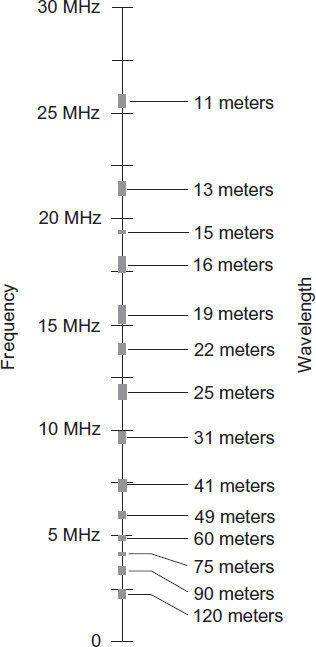
FIGURE 2-4 Nomograph showing the shortwave broadcast bands on a linear scale according to frequency. The frequency increases, and the wavelength gets shorter, as you move upward along the scale.

Other Shortwave Activity

Of course, you’ll find plenty of other activity on the shortwave frequencies besides international broadcasting and ham radio. The NIST broadcasts time and frequency standard signals in the United States from two locations, one in Colorado (WWV) and the other in Hawaii (WWVH). I’ve heard these signals at 5, 10, and 15 MHz quite regularly. Go to the website

www.nist.gov

and do a search on “WWV” as a single word. You’ll find plenty of information about their broadcast format on that site. They do a lot more than provide frequency standards and tell you the time!

As you explore the shortwave realm, you’ll hear strange signals of all sorts: hissing and whining and roaring signals, mostly high-speed digital transmissions along with some jamming signals (yes, that stuff still happens) where one nation doesn’t like what another nation has to say. Many of the signals have a military origin. If you happen to know the Morse code and can “copy” it at a reasonable speed, you might make sense out of some of these signals. My advice here is simple: Get a good general coverage receiver, set up a good antenna as described later in this chapter, and start listening!

A Simple Antenna for SWL

If you buy a commercially manufactured shortwave radio, especially the portable type that seems to prevail these days, it will likely have its own antenna attached: a whip that extends to about one meter in length. That antenna will work okay for receiving strong signals, but your best option for serious SWL is an outdoor random wire at least 20 meters long, and much longer if you can manage it.

Use insulated wire. Plain old lamp cord, also called “zip cord,” works great. So-called “bell wire” also works. String the wire up as high above the ground as you can get it. Connect the far end of the wire to a good ground rod driven into the soil to keep electrostatic charges from building up on the wire. (If you use a copper ground rod, the best kind, make sure it isn’t too close to the roots of any trees or shrubs. Copper can kill plants.)

You can bring the near end of the wire in through a window sash and connect it to the back of your radio (after stripping off the insulation for an inch or so), where you should find a terminal specifically meant for external antennas. If your radio lacks an external antenna terminal and uses an attached collapsible whip antenna instead, strip 3 or 4 inches of insulation off the end of the antenna wire, collapse the whip all the way down except for an inch or two, and wrap the bare conductor around the end of the whip.

You can get enhanced performance if you use a small antenna tuner (also called a transmatch) intended for low-power HF ham radio use. A good source for these devices is a company called MFJ Enterprises. I recommend the model MFJ-16010 or a similar model. It’ll ensure that you get the best possible impedance match between your random wire and your radio. Visit MFJ on the Web at

www.mfjenterprises.com

Never forget to disconnect your outdoor antenna from your radio when you aren’t using the radio. Remove the end of the antenna entirely from the house, and lay it on the ground where nobody can trip over it or otherwise get in trouble with it.

 

Sunspots and Shortwave Radio

The sun’s surface hosts violent storm-like phenomena that we see as sunspots because they radiate less visible light than the rest of the solar disk. You can view sunspots through a telescope equipped with a projection system or a dark filter over the objective lens or opening (never in the eyepiece). A typical sunspot measures farther across than the diameter of the earth! The biggest ones can grow to several earth diameters from one edge to the other. The darkest part of the spot lies at, or near, the center, a region called the umbra. The brighter zone around the umbra constitutes the penumbra, as shown in Fig. 2-5.

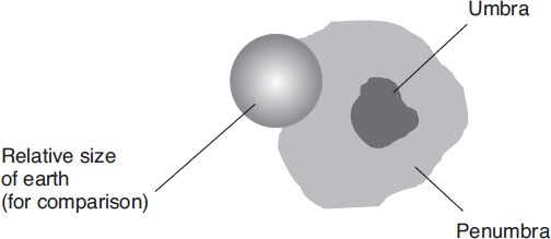
FIGURE 2-5 A typical sunspot has a diameter greater than that of the earth.

Warning! Never view the sun directly through dark film negatives, thinking that the unexposed film will protect your eyes. Ultraviolet rays can penetrate the “celluloid” and do permanent damage to your vision. If you must use a “sun filter,” use one that blocks ultraviolet rays. Don’t use filters that fit in telescope eyepieces; the focused sunlight can heat the filter glass to the point where it breaks, giving your retina a horrific jolt. (As a child, I experienced that mishap and practically fell over backwards! Luckily, I did not suffer permanent eye damage.) Ideally, you should avoid direct sun viewing in any form, and use a telescope projection system that casts an image of the sun on a flat screen.

The Sunspot Cycle

For centuries, astronomers have known that the number of sunspots changes from year to year, month to month, and day to day. Short-term variations can be sporadic, but the long-term fluctuation has a regular and dramatic up-and-down rhythm known as the sunspot cycle. It has a period of approximately 11 years from peak to peak. The actual maxima and minima vary from cycle to cycle. Figure 2-6 shows the sunspot cycles since the year 1920 as a very approximate graph of relative activity versus time. At the time of this writing (2014), the sunspot cycle had passed a peak that was less intense than the several peaks that preceded it.

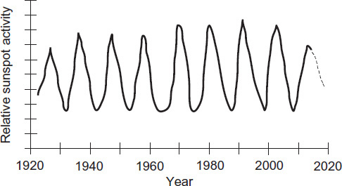
FIGURE 2-6 Approximate graph showing the sunspot cycles that have taken place since 1920.

The amount of radio noise emitted by the sun is called the solar radio-noise flux, or simply the solar flux. Astronomers and communications engineers monitor the solar flux at a wavelength of 10.7 centimeters, corresponding to a frequency of 2800 MHz. At this frequency, the troposphere and ionosphere have minimal effect on radio waves, making observation of extraterrestrial RF phenomena easy. The 2800-MHz solar flux correlates with the sunspot cycle. On the average, the solar flux rises highest near the peak of the sunspot cycle, and dips lowest near sunspot minima.

Maximum Usable Frequency

Imagine some arbitrary medium or high frequency at which communication is possible between two specific points. Now suppose that you increase the frequency gradually until communication fails. This cutoff point is called the maximum usable frequency, or MUF, for the two locations in question.

The MUF depends on the locations and separation distance of the transmitter and receiver. The MUF also varies with the time of day, the season of the year, and the sunspot activity. All of these factors affect the ionosphere. For a given signal path, the propagation usually improves as the frequency rises toward the MUF; at frequencies above the MUF, the “connection” deteriorates.

When you operate a communications circuit slightly below the MUF and then the MUF suddenly drops, a rapid and complete signal fadeout occurs. Long-time users of the HF radio spectrum know all about this effect. If you’ve been a ham radio operator for more than a couple of years, you’ve doubtless witnessed events of this sort. Hams will say that “the band is going out,” or they’ll talk about “QSB” (fading).

Solar Flares

A solar flare is a particularly dramatic eruption on the sun. When viewed through a telescope equipped with the appropriate filters, a solar flare appears as a bright fleck or streamer on the solar disk, thousands of kilometers across and thousands of kilometers high. At any given radio frequency, the solar flux increases abruptly when a solar flare occurs. This effect makes the solar flux useful for propagation forecasting: A sudden increase in the solar flux indicates that ionospheric propagation conditions will likely deteriorate within a few hours. Solar flares can occur at any time, but they take place most often near sunspot cycle peaks.

Solar flares emit countless high-speed atomic particles that hurtle through space at a small fraction of the speed of light, usually reaching the earth several hours after the occurrence of the flare. Because the particles carry an electric charge, they converge toward the earth’s magnetic poles, causing a disturbance in the earth’s magnetic field known as a geomagnetic storm. When that happens, you can see the aurora (northern and southern lights) on clear nights at high latitudes, and shortwave radio reception can fail completely within seconds at all frequencies. Even wire communications circuits sometimes suffer ill effects. In the extreme, the electric utility grid and the Internet can malfunction as well. Scientists don’t know the exact mechanism that causes solar flares, but they can use these events to predict geomagnetic storms.

 

Longwave Radio

Communications specialists call the range of radio frequencies extending from 30 kHz to 300 kHz the low-frequency (LF) or longwave band. Informally, you can think of it as extending from the lowest allocated frequency in the United States at 9 kHz up to the low-frequency end of the standard AM broadcast band at 535 kHz. The wavelengths decrease from 10 kilometers down to 1 kilometer as you go up in frequency from 30 kHz to 300 kHz range. For this reason, some people call LF radio signals kilometric waves.

Waveguide Propagation

The ionosphere’s E and F layers return all LF signals to the earth, even those waves that emanate straight up from the transmitting antenna. Likewise, LF signals of extraterrestrial origin can’t reach us at the earth’s surface because the ionosphere reflects them back into space. In effect, the ionosphere acts as a “radio wave mirror” at these wavelengths.

If you go down low enough in frequency, say to 100 kHz or below, the wavelength gets so long that the earth and the ionosphere combine to act like the surfaces of a transmission line known as a waveguide. Communications engineers and radio hams use waveguides at ultra high and microwave frequencies (300 MHz and above) to carry signals from transmitters to antennas, and/or from antennas to receivers. Physically, a transmission-line waveguide comprises a hollow metal duct or pipe, usually with a rectangular cross section. These transmission lines work with signals whose wavelengths measure millimeters or centimeters. Ionospheric waveguide propagation works with signals whose wavelengths measure kilometers.

In the waveguide mode of propagation, the transmitting antenna, which must produce a vertically polarized EM wave, delivers energy into the space between the earth and ionized layers of the upper atmosphere. The receiving antenna picks up the energy in a manner similar to an RF probe in an electronics lab. The earth-ionosphere waveguide has a minimum-frequency cutoff (lower limit) of around 9 kHz. At lower frequencies, signals don’t propagate well because the wavelength is too long to let the earth and the ionosphere function properly as a waveguide. In fact, the earth-ionosphere waveguide effectively shorts out EM fields at frequencies below about 9 kHz, and that’s why those frequencies remain largely ignored for use on this planet. (At the time of this writing, frequencies below 9 kHz were not legally allocated for any purpose in the United States.)

Waveguide propagation occurs along with surface-wave propagation, which you learned about in Chap. 1.

Maximum Usable Low Frequency

For any two points separated by more than a few kilometers, radio communication works well only at certain frequencies. At the longest wavelengths in the LF band, and also in the very-low-frequency (VLF) band below 30 kHz, communications circuits will almost always function worldwide, as long as the transmitter puts out enough RF power and the receiver has optimum selectivity and noise rejection capability.

Imagine a working communications circuit at a frequency of a few kilohertz between two specific points on the earth’s surface. Suppose that you gradually raise the frequency. If the transmitter and the receiver are more than a few kilometers apart, the path loss (the difficulty with which signals propagate by means of surface-waves or waveguide mode) increases as the frequency goes up. This effect occurs because the lowest layer of the ionosphere becomes less reflective and more absorptive as the frequency rises, and also because the ground becomes less conductive so that the surface wave can’t propagate as well. Under some conditions, you’ll encounter a frequency at which communication deteriorates to the point of uselessness. This frequency will lie far below the useful shortwave communications range between the same two points. Engineers call this point in the LF band the maximum usable low frequency (MULF).

The MULF differs from the shortwave MUF. If you raise the frequency above the MULF, communication will not take place for a while, but if you keep going, you’ll establish a working circuit once again (between the same two points) at a frequency called the lowest usable high frequency (LUHF). As the frequency increases still more, as you’ve learned, the circuit will fail again at the shortwave MUF.

How to Get Down There

If you want to listen to signals at frequencies below the standard AM broadcast band (535 kHz in the United States), you’ll need a receiver that can tune through that range. Most older shortwave radios can’t do it. For example, my 1960s Hallicrafters radio would only go down to the bottom of the AM broadcast band. However, many modern radios can “hear” almost all the way down to the audio frequency (AF) zone, which tops out around 20 kHz. A typical lower limit for such receivers is 30 kHz, the bottom of the LF band, corresponding to a free-space wavelength of 10 kilometers.

My own ham radio transceiver (Fig. 2-7) can receive signals down to 30 kHz and also up to 174 MHz, a frequency that lies well into the VHF part of the radio spectrum. (It can transmit only within the Amateur Radio bands that existed in the United States at the time of its manufacture around 2001.) Most other good HF ham “rigs” can do the same thing. It’s a great feature, because you don’t have to buy a separate shortwave radio. The versatility and signal-refining capabilities of a good HF ham radio compare favorably with the best dedicated allwave receivers.

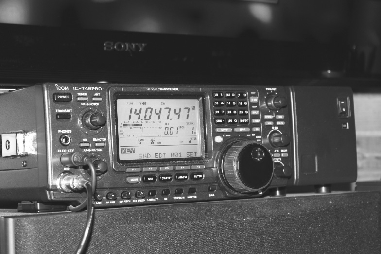
FIGURE 2-7 Most Amateur Radio HF transceivers cover a wide range of frequencies for reception with precision and flair! Here’s an example: My own fixed-station ham radio set, which can tune continuously from 30 kHz to 174 MHz.

Whatever type of radio you use, you’ll need a good antenna in order to effectively receive signals at long wavelengths. In general, as the wavelength gets longer, efficient transmitting antennas grow larger in commercial applications. There’s no way around that conundrum: a decent radiating element for LF use must be large, indeed, and high up off the ground to boot. For receiving, things are a lot simpler. You’ll find two types of receiving antennas in common use at LF and also at VLF:

   1. A random wire, of indeterminate length (but as long as possible), strung up outdoors as high above the ground as you can place it; or

   2. A small loop antenna with a tuning capacitor or preamplifier to boost the signal level, used indoors next to the radio.

The first type of LF and VLF listening antenna, the outdoor long wire, pretty much explains itself in terms of design. If you have a lot of real estate available (for example, if you live on a farm or ranch), consider yourself blessed! Put the antenna up between the tallest supports you can find, such as big trees. If you don’t have any big trees on your property, you can put up masts or towers to serve as antenna supports. You can string the wire up between more than two supports, and it doesn’t have to go in a straight line. The most important consideration is that your wire sit up in the clear, away from obstructions, and that you avoid placing it in such a way that it can fall or blow down on an electric utility line, or that an electric utility line can fall or blow down on it. You can run the wire down into your house through an open window, slam the window shut on the wire, and then connect the end of the wire to the antenna terminal on the back of the radio.

Warning! Any outdoor antenna presents a danger when thunderstorms occur in your vicinity. As you make your wire antenna longer, the danger increases because it will readily accumulate massive electrostatic charges. A storm doesn’t have to be overhead in order to put your radio, your home, and your life at risk. Even when a thunderstorm is several kilometers away, it can “charge up the atmosphere” enough to electrify a long wire antenna to an astonishing extent. You must connect your antenna to a good ground, preferably a long copper rod (2 meters or more) driven into good soil and placed at least 10 or 15 meters from your house, whenever you aren’t using the radio. When you do use it, make sure that no thunderstorms exist anywhere nearby. You might want to keep a computer on one of the Internet radar sites so that if a storm approaches or rapidly develops, you can “see” it coming.

The second type of LF and VLF listening antenna in common use, the small loop, works according to the principle of “grabbing the magnetic component” of the EM field. Figure 2-8 shows the basic configuration. It should have an overall circumference of less than 0.1 wavelength (that’s right, less!) at the highest operating frequency. It can be circular or square in shape. Such an antenna exhibits a sharp null (zone of minimum sensitivity) along the loop axis. At LF and VLF, a small loop must contain numerous turns of wire; as the frequency goes down, the number of required turns goes up. A variable capacitor, in conjunction with the coil, forms an RF tuned circuit. You set the loop’s optimum receiving frequency by adjusting the capacitor.

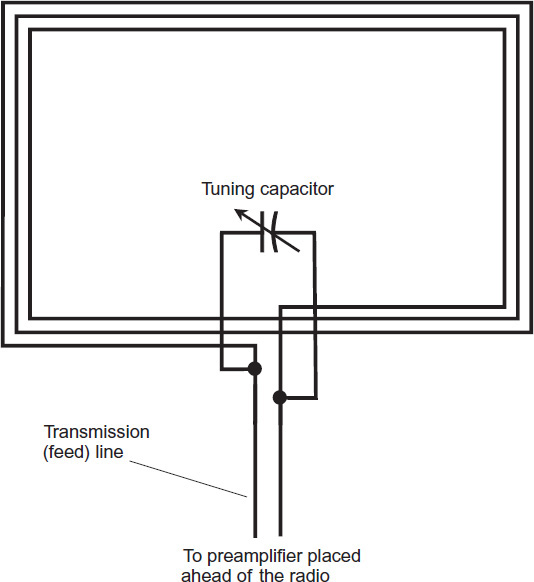
FIGURE 2-8 A small loop antenna for receiving LF signals. The loop contains several turns and can have a diameter of about 1 meter. The variable capacitor allows you to tune the system to resonance (optimum signal conditions) at the desired frequency.

For compactness and convenience, and also to increase the loop inductance, a length of insulated or enameled wire can be wound around a rod-shaped inductor core made of powdered iron. This type of antenna, called a loopstick, has directional characteristics similar to the ordinary small loop. The sensitivity is maximum off the sides of the coil, and a sharp null occurs off the ends. Instead of (or in addition to) using a tuning capacitor, you can insert a tunable RF preamplifier between the loop and the receiver’s front end or antenna input. That device will give you some extra sensitivity and selectivity for bringing in the weakest signals and reducing interference from the strongest ones.

LowFERs

If you have a lot of patience, a sensitive LF receiver, and a well-engineered receiving antenna in a good location, you might hear signals from people who engage in a hobby called LowFER (an acronym that stands for low frequency experimental radio) in the longwave frequency range between 160 kHz and 190 kHz. The actual wavelengths go from 1875 meters down to 1579 meters, and you’ll hear enthusiasts refer to this slot of the spectrum in general terms as the 1750-meter band. In addition to checking out the experimenters on 1750 meters, you might tune down in frequency a little ways and hear ham radio experimenters testing low-power transmitters on 136 kHz (2206 meters).

You don’t need a license in the United States in order to conduct LowFER activities that involve transmitting between 160 kHz and 190 kHz, as long as you adhere to certain restrictions. (You must have a ham radio license to conduct experiments that involve transmitting on 136 kHz.) For LowFER operation, you can’t use a transmitting antenna with an overall length that exceeds 15.24 meters, including the transmission line between the radio and the radiating element itself. In addition, your transmitter can’t have an RF power output that exceeds 1 watt. On account of these severe restrictions, most LowFERs use Morse code or digital modes for communication in order to ensure that people listening for them get to take advantage of the best possible signal-to-noise (S/N) ratio.

If you get lucky, you might hear a LowFER or two sending experimental signals from a few hundred kilometers away. Maybe you’ll want to get on the air as a LowFER and see if you can make two-way contacts with other LowFERs! For more information about this hobby, visit the website of the Longwave Club of America (LWCA) at

www.lwca.org

Converters for VLF

If you want to listen to signals at frequencies below 30 kHz and your receiver can’t do it, you can build a converter that will let you listen all the way down to DC (0 Hz), at least in theory. (In practice, noise and the converter’s own oscillator make reception difficult below about 3 kHz.) Figure 2-9 is a generic diagram of a VLF converter that mixes incoming VLF signals with an unmodulated carrier from a local oscillator at some frequency in the shortwave band, such as 3500 kHz. The circuit produces, in effect, a wideband AM signal with sidebands that extend several tens of kilohertz above and below that frequency. You can use a shortwave radio receiver to tune through those sidebands and hear VLF signals at the sum and difference frequencies. For example, a VLF signal coming in at 17 kHz would show up in the receiver at 3517 kHz (3500 + 17) and also at 3483 kHz (3500 − 17).

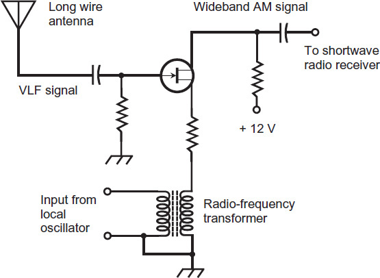
FIGURE 2-9 Generic diagram of a VLF converter. Exact component values must be determined by experimentation.

 

Dirty Electricity

As you learned in Chap. 1, electric and magnetic flux lines surround all current-carrying wires. Around a straight wire, the electric or E flux lines run parallel to the wire, and the magnetic or M flux lines encircle the wire, as shown in Fig. 2-10A. If the wire carries constant DC, the E and M fields remain constant and steady. If the wire carries AC or pulsating DC, the fields fluctuate, producing an EM field that emanates from the wire. At great distances from the wire, the E and M lines of flux are perpendicular to each other in a nearly flat plane, forming an EM field that travels through space at the speed of light, as shown in Fig. 2-10B. This field induces AC in any nearby object that conducts electricity, such as your radio antenna. Unfortunately, any nearby AC utility line or house wiring produces EM energy not only at 60 Hz, but also at harmonics (whole-number multiples) of 60 Hz, as well as at other unrelated frequencies. The spectrum below a few kilohertz suffers from “EM pollution” on account of this dirty electricity in any area served by an electric utility. At LF and especially at VLF, you’ll notice the effects as soon as you tune a radio down there. The EM waves that you want to hear, and the ones that you don’t want to hear, both originate and propagate in the same way, as Figs. 10A and 10B show. In a city, dirty electricity can render VLF reception impossible. Not only can you hear this stuff, but also, with the appropriate equipment, you can see it too! Here’s how you can put together a device that will detect dirty electricity and produce a graphic display of its characteristics (although it won’t help you get rid of it).

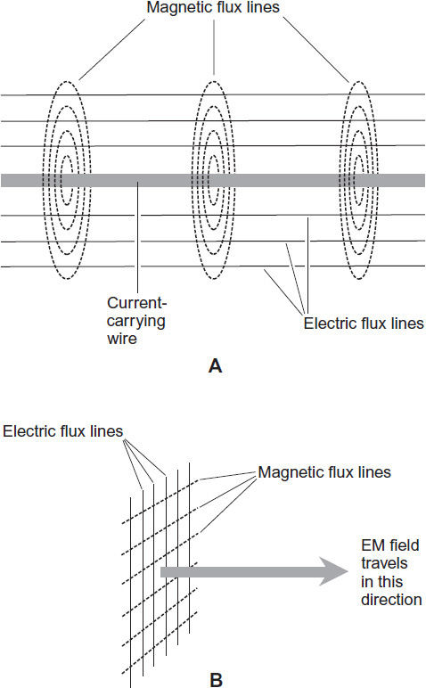
FIGURE 2-10 At A, the electric (E) and magnetic (M) lines of flux around a straight, current-carrying wire. At B, the flux lines far away from a current-carrying wire.

A Cool Little Program

A simple freeware program called DigiPan, available on the Internet, can provide a real-time, moving graphical display of EM field components at frequencies ranging from 0 Hz (that is, DC) up to around 5500 Hz. Here’s the website:

www.digipan.net

DigiPan shows the frequency along a horizontal axis, while time is portrayed as downward movement all across the whole display. Figure 2-11 shows this scheme. The relative intensity at each frequency appears as a color. You can adjust the colors to suit your taste. If no energy exists at any frequency in the program’s range, the display will appear completely black. If there’s a little bit of energy at a particular frequency, you’ll see a thin, vertical blue line creeping straight downward (if you leave the program set for its default color scheme). If there’s a moderate amount of energy, the line turns yellow. If there’s a lot of energy, the line becomes orange or red. The developers and users of DigiPan and similar programs have coined the term waterfall for the display, because of its appearance when signals exist at numerous frequencies.

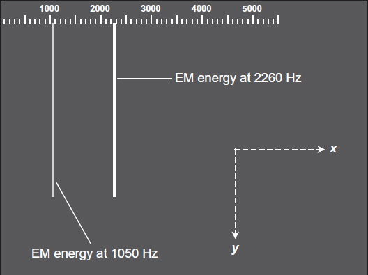
FIGURE 2-11 Basic geometrical scheme for the DigiPan display. The horizontal axis portrays frequency. Time “flows” downward across the whole screen. Signals show up as vertical lines. This drawing shows two hypothetical examples.

The Hardware

To observe dirty electricity on your computer, you’ll need an “antenna” that can “pick up the trash.” Get an audio cord at least 3 meters long with a mini two-wire (monaural) phone plug on one end and spade lugs on the other. Cut off the U-shaped spade lugs from the audio cord with a scissors or diagonal cutter. Separate the wires by pulling them apart along the entire length of the cord so that you get a phone plug with two wires attached, forming a little dipole antenna.

Insert the phone plug into the microphone input of your computer. Arrange the two wires so that they run in different directions from the phone plug. You can let the wires lie anywhere, as long as you don’t trip over them! This arrangement will make the audio cord pick up EM energy.

Open the audio control program on your computer. If you see a microphone input volume or sensitivity control, set it to maximum. Set your computer to work with an external microphone, not the internal one. If your audio program has a “noise reduction” feature, turn it off. Set the microphone gain (or input sensitivity) to maximum. Then launch DigiPan and follow these steps, in order.

     • Click on “Options” in the menu bar and uncheck everything except “Rx.”

     • Click on “Mode” in the menu bar and select “BPSK31.”

     • Click on “View” in the menu bar and uncheck everything.

Once you’ve carried out these steps, the upper part of your computer display should show a jumble of text characters on a white background. The lower part of the screen should be black with a graduated scale at the top, showing the numerals 1000, 2000, 3000, and so on. Using your mouse, place the pointer on the upper border of the black region and drag that border upward until the white region with the distracting text vanishes.

If things work correctly, you should have a real-time panoramic display of EM energy from zero to several thousand hertz. Unless you’re in a remote location far away from the utility grid, you should see vertical lines of various colors. These lines represent EM energy components at specific frequencies. You can read the frequencies from the graduated scale at the top of the screen. Do you notice a pattern?

Harmonics

A pure AC sine wave appears as a single pip or vertical line on the display of a spectrum monitor (Fig. 2-12A). This pip means that all of the energy in the wave is concentrated at one frequency, known as the fundamental frequency. But many, if not most, AC utility waves contain harmonic energy along with the energy at the fundamental frequency.

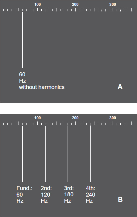
FIGURE 2-12 At A, a spectral diagram of pure, 60-Hz EM energy. At B, a spectral diagram of 60-Hz energy with significant components at the second, third, and fourth harmonic frequencies.

A harmonic is a whole-number multiple of the fundamental frequency. For example, if 60 Hz is the fundamental frequency, then harmonics can exist at 120 Hz, 180 Hz, 240 Hz, and so on. The 120-Hz wave is at the second harmonic, the 180-Hz wave is at the third harmonic, the 240-Hz wave is at the fourth harmonic, and so on. In general, if a wave has a frequency equal to n times the fundamental frequency where n is some whole number, then that wave is called the nth harmonic. (The fundamental frequency is the first harmonic by definition). In Fig. 2-12B, a wave is shown along with its second, third, and fourth harmonics, as the entire “signal” would appear on a spectrum monitor.

When you look at the EM spectrum display from zero to several thousand hertz using DigiPan, you’ll see that utility AC energy contains not only the 60-Hz fundamental, but also many harmonics. When I saw how much energy exists at the harmonic frequencies in and around my house, my astonishment knew no bounds. I had suspected “dirt in the ether,” but not that much! Figure 2-13 shows my own DigiPan display of dirty electricity from 60 Hz to more than 4000 Hz in the workspace where I wrote this book. Each vertical trace represents an EM signal at a specific frequency. If the electricity were “perfectly clean,” you’d see only one bright vertical trace at the extreme left end of the display.

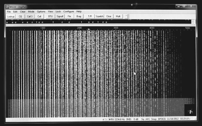
FIGURE 2-13 Dirty electricity in my work space, as viewed on DigiPan.

Try This Circuit for Relief!

You might be able to reduce the noise from dirty electricity at frequencies below about 100 kHz by using two antennas that receive the noise at equal amplitudes but receive the desired signals at different amplitudes. You must connect the two antennas together so the noise signals cancel each other out. Figure 2-14 shows an example of a circuit that I have used to accomplish this feat. With a little testing and tweaking, maybe you can make it work too.

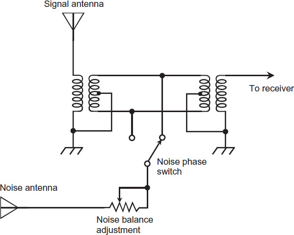
FIGURE 2-14 A noise-canceling antenna scheme that works especially well at VLF.

In order for a circuit of this sort to function at its best, the signal antenna and the noise antenna must lie reasonably near each other, so they pick up local humanmade noise whose characteristics are as nearly identical as possible. But they should not be too close together, or the desired signals will get canceled along with the noise. Place the signal antenna in a location favorable for the reception of the stuff you want to hear, and locate the noise antenna so that it will receive as much dirty electricity as possible (and relatively little of the desired signals). For example, the signal antenna might be a tall vertical element operating against an earth ground; the noise antenna can comprise a short, random length of wire run on the floor inside your house.

The potentiometer lets you adjust the level of signals and noise from the noise antenna, while having a minimal effect on the overall signal level from the two antennas combined. The phase switch allows for injection of the noise from the noise antenna either “right side up” or “upside down,” so that you can make sure that it enters the rest of the circuit in phase opposition with the noise from the signal antenna. At frequencies below approximately 30 kHz, where wavelengths are measured in kilometers, the noise from the two antennas will be either coincident in phase or opposite in phase. After you have found the correct switch position by trial and error, adjust the potentiometer until you get minimum “trash” in your receiver.

When I first put this circuit together, I didn’t know how well it would work. I was astonished when I saw the noise go from over S-9 on my receiver signal meter down to only about S-3! That’s a reduction of six S units, where each S unit (on most receivers) represents about 5 dB. If you take it as 5 dB, then you can see that I got a 30-dB improvement with the noise-canceling antenna system, which means that the noise power at my receiver’s “antenna terminals” (T-4X microphone jack) went down to only 1/1000 of its previous level. The desired signals, however, remained as strong as ever.

I have used this scheme for receiving signals at VLF, in conjunction with a VLF converter and a shortwave receiver, with excellent results. The signal antenna was a 16-foot, ground-mounted vertical antenna fed with coaxial cable, intended mainly for operation on the 14-MHz ham radio band. The noise antenna was wire a few feet long, running under a rug on the hallway floor.

As you increase the frequency above the VLF band, this scheme gets less effective because the noise impulses at the two antennas are no longer exactly in phase coincidence or phase opposition unless the antennas are so close together that the circuit cancels the desired signals as well as the noise. In addition, I have found that this circuit does not work against sferics (thunderstorm “static”).

 

Which Radio’s for You?

If you want to get into SWL or AWL, you can buy a ready-made receiver, buy a kit that you can assemble into a receiver, or build your own radio from scratch. The best commercially manufactured radios can run you upwards of a thousand dollars; the cheapest kits or “mini radios” might cost you only $30 or $40.

I won’t attempt to make any product comparisons or recommendations here. Shortwave and allwave receiver designs and features keep changing, almost from day to day. By the time you read anything specific that I might quote, you’d have good reason to suspect that the information had already grown obsolete!

If you want to get into SWL or AWL with a reasonably good radio right away, I recommend that you go to your local Radio Shack store and shop around. If they don’t have physical units right on their shelves, go to the Radio Shack website and you’ll find a wide range of models, one of which will surely suit your desires! Their home page is at

www.radioshack.com

May I also suggest that you attend a meeting of a local ham radio club, or stop by one of the hundreds of ham radio conventions that take place nationwide? They’ll provide all sorts of advice and insights— and they’ll probably try to get you interested in their hobby as well. If you get interested in ham radio and decide to go for a license so that you can create signals as well as merely listen to them, trust me: You’ll be glad you did.