FEM for 3D Solid Elements
9.1 Introduction
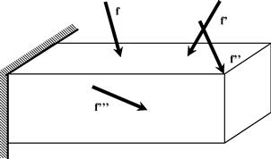
A three-dimensional (3D) solid element can be considered to be the most general of all solid finite elements because the field variables are described fully in terms of all three physical coordinates: x, y, and z. An example of a 3D solid structure under loading is shown in Figure 9.1, where the force vectors are described arbitrarily in any spatial direction. A 3D solid can also have any arbitrary shape, material properties, and boundary conditions in space. As such, there are a total of six possible stress components, three normal and three shear, that need to be taken into consideration. Typically, a 3D solid element can be tetrahedron or hexahedron in shape with either flat or curved surfaces. Each node of the element will have three translational degrees of freedom (DOFs). The element can thus deform in all three directions in space.
Since the 3D element is considered the most general solid element, the truss, beam, plate, 2D solid and shell elements can all be considered to be special cases of the 3D element. So, why is there a need to develop all the other elements covered in previous chapters? Why not just use the 3D elements to model everything? Theoretically, yes, the 3D element can actually be used to model all kinds of structural components including trusses, beams, plates, shells, and so on. However, it can be very tedious in geometry creation and meshing. Furthermore, it is also the most demanding on computer resources. Hence, the general rule of thumb is, when a structure can be assumed within acceptable tolerances to be simplified into a 1D (trusses, beams, and frames) or 2D (2D solids and plates) structure, we shall always do so. The creation of 1D or 2D FEM models is very much easier and more efficient. We use 3D solid elements only when we have no other choices. The formulation of 3D solid elements is straightforward, because it is basically an extension of 2D solid elements. All the techniques used in 2D solids can be utilized, except that all the variables are now functions of x, y, and z. The basic concepts, procedures, and formulations for 3D solid elements may be found in many existing books (see, for example, Washizu, 1981; Rao, 1999; Zienkiewicz and Taylor, 2000).
9.2 Tetrahedron element
9.2.1 Strain matrix
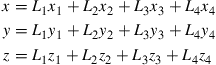
Consider the same 3D solid structure as Figure 9.1, whose domain is divided in a proper manner into a number of tetrahedron elements with four nodes and four surfaces, as shown in Figure 9.2. A tetrahedron element has four nodes and each node has three DOFs (u, v, and w), which makes the total DOFs in a tetrahedron element twelve, as shown in Figure 9.3. The nodes are numbered 1, 2, 3, and 4 by the right- hand rule. The local Cartesian coordinate system for a tetrahedron element can usually be the same as the global coordinate system, as there are no advantages in having a separate local Cartesian coordinate system. In an element, the displacement vector U is a function of the coordinate x, y, and z, and is interpolated by shape functions in the following form, which should be, by now, part and parcel of the finite element method.
![]() (9.1)
(9.1)
where the nodal displacement vector, de, is given as and the matrix of shape functions has the form To develop the shape functions, we make use of what are known as the volume coordinates, which are a natural extension from the area coordinates for 2D solids. The use of the volume coordinates makes it more convenient for shape function construction and element matrix integration. The volume coordinates for node 1 are defined as
 (9.2)
(9.2)
 (9.3)
(9.3)
![]() (9.4)
(9.4)
where VP234 and V1234 denote, respectively, the volumes of the tetrahedrons P234 and 1234, as shown in Figure 9.4. The volume coordinate for node 2–4 can also be defined in the same manner.
![]() (9.5)
(9.5)
The volume coordinate can also be viewed as the ratio between the distance of the point P and point 1 to the plane 234.
![]() (9.6)
(9.6)
It can easily be confirmed that
![]() (9.7)
(9.7)
since
![]() (9.8)
(9.8)
It can also easily be confirmed that
 (9.9)
(9.9)
Using Eq. (9.9) above, the relationship between the volume coordinates and the Cartesian coordinates can be easily derived.
 (9.10)
Equations (9.7) and (9.10) can then be expressed as a single matrix equation as follows:
 (9.11)
The inversion of Eq. (9.11) above will give
 (9.12)
where
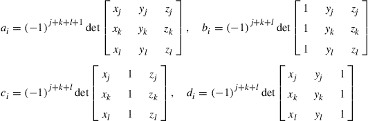 (9.13)
in which the subscript i varies from 1 to 4, and j, k, and l are determined by a cyclic permutation in the order of i, j, k, l. For example, if i = 1, then j = 2, k = 3, l = 4. When i = 2, then j = 3, k = 4, l = 1. The volume of the tetrahedron element V can be obtained by
 (9.14)
The properties of Li as depicted in Eqs. (9.6) to (9.9) show that Li can be used as the shape function of a 4-nodal tetrahedron element.
![]() (9.15)
(9.15)
It can be seen from above that the shape function is a linear function of x, y, and z, hence, the 4-nodal tetrahedron element is a linear element. Note that from Eq. (9.14), the moment matrix of the linear basis functions will never be singular, unless the volume of the element is zero (or the four nodes of the element are in a plane). Based on Lemma 2 and 3 in Chapter 3, we can ensure that the shape functions given by Eq. (9.15) satisfy sufficiently the requirement of FEM shape functions.


It was mentioned that there are a total of six stress components in a 3D element. The stress components can be written in a vector form as
![]()
To get the corresponding vector of strain components,
![]()
we can substitute Eq. (9.1) into Eq. (2.5) from Chapter 2.
![]() (9.16)
(9.16)
where the strain matrix B is given by
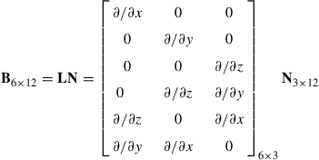 (9.17)
Substituting Eq. (9.3) into the above, the strain matrix B can be obtained as
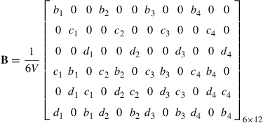 (9.18)
It can be seen that the strain matrix for a linear tetrahedron element is a constant matrix. This implies that the strain within a linear tetrahedron element is constant, and thus the stress is also constant. Therefore, the linear tetrahedron elements are also often referred to as a constant strain element or constant stress element, similar to the case of 2D linear triangular elements.
9.2.2 Element matrices
Once the strain matrix is obtained, the stiffness matrix ke for 3D solid elements can be obtained by substituting Eq. (9.18) into Eq. (3.71) from Chapter 3. Since the strain is constant, the element stiffness matrix is obtained as
![]() (9.19)
(9.19)
Note that the material constant matrix c is given generally by Eq. (2.9) in Chapter 2.
The mass matrix can similarly be obtained using Eq. (3.75) from Chapter 3.
 (9.20)
where
 (9.21)
Using the following formula (Eisenberg and Malvern, 1973) for volume coordinates,
![]() (9.22)
(9.22)
we can conveniently evaluate the integral in Eq. (9.20) to give
 (9.23)
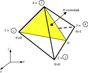
An alternative way to calculate the mass matrix for 3D solid elements is to use a special natural coordinate system, which is defined as shown in Figures 9.5, 9.6 and 9.7. In Figure 9.5, the plane of ξ = constant is defined in such a way that the edge P-Q stays parallel to the edge 2–3 of the element, and the point 4 coincides with point 4 of the element. When P moves to point 1, ξ = 0, and when P moves to point 2, ξ = 1. In Figure 9.6, the plane of η = constant is defined in such a way that the edge 1–4 on the triangle coincides with the edge 1–4 of the element, and point P stays on the edge 2–3 of the element. When P moves to point 2, η = 0, and when P moves to point 3, η = 1. The plane of ζ = constant is defined in Figure 9.7, in such a way that the plane P-Q-R stays parallel to the plane 1–2–3 of the element, and when P moves to point 4, ζ = 0, and when P moves to point 2, ζ = 1. In addition, the plane 1–2–3 on the element sits on the x–y plane. Therefore, the relationship between xyz and ξηζ can be obtained in the following steps:


In Figure 9.8, the coordinates at point P are first interpolated using the x, y, and z coordinates at points 2 and 3:
 (9.24)
The coordinates at point B are then interpolated using the x, y, and z coordinates at points 1 and P:
 (9.25)
The coordinates at point O are finally interpolated using the x, y, and z coordinates at points 4 and B:
 (9.26)
With this special natural coordinate system, the shape functions in the matrix of Eq. (9.3) can be written by inspection as
 (9.27)
The Jacobian matrix between xyz and ξηζ is required and is given as
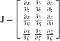 (9.28)
Using Eqs. (9.26) and (9.27), the determinate of the Jacobian can be found to be
![]() (9.29)
(9.29)
The mass matrix can now be obtained as
![]() (9.30)
(9.30)
which gives
 (9.31)
where Nij is given by Eq. (9.21), but in which the shape functions should be defined by Eq. (9.27). Evaluating the integrals in Eq. (9.31) would give the same mass matrix as in Eq. (9.23).

The nodal force vector for 3D solid elements can be obtained using Eqs. (3.78), (3.79) and (3.81). Suppose the element is loaded by a distributed force fs on the edge 2–3 of the element as shown in Figure 9.3, the nodal force vector becomes
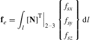 (9.32)
If the load is uniformly distributed, fsx, fsy, and fsz are constants and the above equation becomes
 (9.33)
where l2–3 is the length of the edge 2–3. Eq. (9.33) implies that the distributed forces are equally divided and applied at the two nodes. This conclusion applies also to evenly distribute surface forces applied on any face of the element, and to evenly distribute body force applied on the entire body of the element. Finally, the stiffness matrix, ke, the mass matrix, me, and the nodal force vector, fe, can be used directly to assemble the global FE equation, Eq. (3.96), without going through a coordinate transformation.
9.3 Hexahedron element
9.3.1 Strain matrix
Consider now a 3D domain, which is divided in a proper manner into a number of hexahedron elements with eight nodes and six surfaces, as shown in Figure 9.9. Each hexahedron element has nodes numbered 1, 2, 3, 4 and 5, 6, 7, 8 in a counter-clockwise manner, as shown in Figure 9.10.


As there are three DOFs at one node, there are now a total of twenty-four DOFs in a hexahedron element. It is again useful to define a natural coordinate system (ξ, η, ζ) with its origin at the center of the transformed cube, as this makes it easier to construct the shape functions and to evaluate the matrix integration. The coordinate mapping is performed in a similar manner to that of quadrilateral elements in Chapter 7. Like the quadrilateral element, shape functions are also used to interpolate the coordinates from the nodal coordinates:
 (9.34)
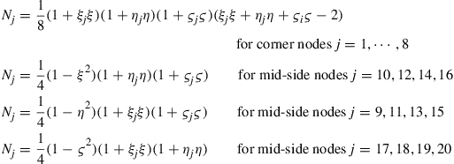
The shape functions are given in the local natural coordinate system as
 (9.35)
![]() (9.36)
(9.36)
where (ξi, ηi, ζi) denotes the natural coordinates of node i.
From Eq. (9.36), it can be seen that the shape functions vary linearly in each of the ξ, η, and ζ directions. Therefore, these shape functions are sometimes called trilinear functions. The shape function Ni is a three-dimensional analogy of that given in Eq. (7.54). It can be shown through direct observation that the trilinear elements possess delta function property. In addition, since all these shape functions can be formed using the common set of 8 basis functions of
![]() (9.37)
(9.37)
which contain both constant and linear basis functions, these shape functions can expect to possess both partitions of unity property as well as the linear reproduction property (see Lemma 2 and 3 described in Chapter 3).
In a hexahedron element, the displacement vector U is a function of the coordinates x, y, and z, and like before, it is interpolated using the shape functions:
![]() (9.38)
(9.38)
where the nodal displacement vector, de, is given by
 (9.39)
in which,
 (9.40)
is the displacement at node i. The matrix of shape functions is given by
![]() (9.41)
(9.41)
in which each sub-matrix, Ni, is given as
 (9.42)
In this case, the strain matrix defined by Eq. (9.17) can be expressed as
![]() (9.43)
(9.43)
whereby
 (9.44)
As the shape functions are defined in terms of the natural coordinates, ξ, η, and ζ, to obtain the derivatives with respect to x, y, and z in the strain matrix, the chain rule of partial differentiation needs to be used:
 (9.45)
which can be expressed in the matrix form of
 (9.46)
where J is the Jacobian matrix defined by
 (9.47)
Recall that the coordinates, x, y, and z are interpolated by the shape functions from the nodal coordinates. Hence, substituting the interpolation of the coordinates, Eq. (9.34) into Eq. (9.47) above gives
 (9.48)
or
 (9.49)
Equation (9.46) can be re-written as
 (9.50)
which is then used to compute the strain matrix, B, in Eqs. (9.43) and (9.44), by replacing all the derivatives of the shape functions with respect to x, y, and z to those with respect to ξ, η, and ζ.
9.3.2 Element matrices
Once the strain matrix, B, is computed, the stiffness matrix, ke, for 3D solid elements can be obtained by substituting B into Eq. (3.71) from Chapter 3.
![]() (9.51)
(9.51)
Note that the matrix of material constant, c, is given by Eq. (2.9) from Chapter 2. As the strain matrix, B, is a function of ξ, η, and ζ, evaluating the integrations in Eq. (9.51) can be tedious. Therefore, the integrals are performed using a numerical integration scheme. The Gauss integration scheme discussed in Section 7.3.4 of Chapter 7 is often used to carry out the integral. For three-dimensional integrations, the Gauss integration is sampled in three directions as follows:
 (9.52)
To obtain the mass (inertia) matrix for the hexahedron element, substitute the shape function matrix, Eq. (9.41), into Eq. (3.75) from Chapter 3.
![]() (9.53)
(9.53)
The above integral is also usually carried out using the Gauss integration. If the hexahedron is rectangular with dimensions of 2a × 2b × 2c, the determinate of the Jacobian matrix is simply given by
![]() (9.54)
(9.54)
and the mass matrix can be explicitly obtained as
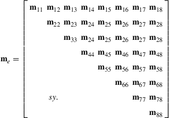 (9.55)
 (9.56)
or
 (9.57)
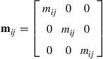
in which,
 (9.58)
As an example, m33 is calculated as follows:
![]() (9.59)
(9.59)
The other components of the mass matrix for a rectangular hexahedron element are thus
 (9.60)
Note that the equalities in the above equation can be easily figured out by observing the relative geometric positions of the nodes in the cube element. For example the relative geometric positions of nodes 1–2 are equivalent to the relative geometric positions of nodes 2–3, and the relative geometric positions of nodes 1–7 are equivalent to the relative geometric positions of nodes 2–8. If we write the portion of the mass matrix corresponding to only one translational direction, say the x direction, we have
 (9.61)
The mass matrices corresponding to only the y and z directions are exactly the same as me.
The nodal force vector for a rectangular hexahedron element can be obtained using Eqs. (3.78), (3.79), and (3.81). Suppose the element is loaded by a distributed force fs on the edge 3–4 of the element, as shown in Figure 9.10, the nodal force vector becomes
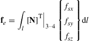 (9.62)
If the load is uniformly distributed and fsx, fsy, and fsz are constants, then the above equation becomes:
 (9.63)
where l3–4 is the length of the edge 3–4. Eq. (9.63) implies that the distributed forces are equally divided and applied at the two nodes. This conclusion also applies to evenly distributed surface forces applied on any face of the element, and to evenly distributed body force applied on the entire body of the element.
9.3.3 Using tetrahedrons to form hexahedrons
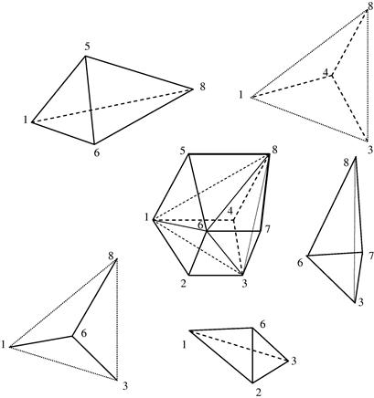
An alternative method of formulating hexahedron elements is to make use of tetrahedron elements. This is built upon the fact that a hexahedron can be said to be made up of numerous tetrahedrons. Figure 9.11 shows how a hexahedron can be made up of five tetrahedrons. Of course, the way a hexahedron can be made up of five tetrahedrons is not unique and, in fact, it can also be made up of six tetrahedrons as shown in Figure 9.12. Similarly, there is more than one way of dividing a hexahedron into six tetrahedrons. In this way, the element matrices for a hexahedron can be formed by assembling all the matrices for the tetrahedron elements, each of which is developed in Section 9.2. The assembly is done in a similar way as the assembly between elements.

9.4 Higher order elements
9.4.1 Tetrahedron elements
Two higher order tetrahedron elements with 10 nodes and 20 nodes are shown in Figure 9.13a and b, respectively. The 10-node tetrahedron element is a quadratic element. Compared with the linear tetrahedron element (4-nodal) developed earlier, six additional nodes are added at the middle of the edges of the element. In developing the 10-nodal tetrahedron element, a complete polynomial up to second order can be used. The shape functions for this quadratic tetrahedron element in the volume coordinates are given as follows:
 (9.64)
where Li is the volume coordinate, which is the same as the shape function for the linear tetrahedron elements given by Eq. (9.15).

Figure 9.13 Higher order 3D tetrahedron elements. (a) 10-node tetrahedron element; (b) 20-node tetrahedron element.
The 20-node tetrahedron element is a cubic element. Compared with the linear tetrahedron element (4-nodal) developed earlier, two additional nodes are added evenly on each edge of the element, and 4 central-face nodes are added at the geometry center of each triangular surface of the element. In developing the 20-nodal tetrahedron element, a complete polynomial up to third order can be used. The shape functions for this cubic tetrahedron element in the volume coordinates are given as follows:
 (9.65)
where Li is the volume coordinate, which is the same as the shape function for the linear tetrahedron elements given by Eq. (9.15).
9.4.2 Brick elements
9.4.2.1 Lagrange type elements
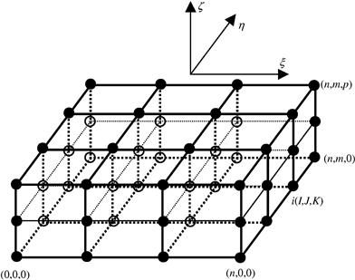
The Lagrange type brick elements can be developed in precisely the same manner as the 2D rectangular elements described in Chapter 7. A brick element with nd= (n+1)(m+1)(p+1) nodes is shown in Figure 9.14. The element is defined in the domain of (−1 ≤ξ ≤1, −1 ≤ η ≤1, −1 ≤ζ ≤1) in the natural coordinates ξ, η, and ζ. Due to the regularity of the nodal distribution along ξ, η, and ζ directions, the shape function of the element can be simply obtained by multiplying one-dimensional shape functions with respect to ξ, η, and ζ directions using the Lagrange interpolants defined in Eq. (4.73) (Zienkiewicz et al., 2000).
![]() (9.66)
(9.66)
Due to the delta function proper of the 1D shape functions given in Eq. (4.74), it is easy to confirm that Ni given by Eq. (9.66) also possesses the delta function property.
9.4.2.2 Serendipity type elements
The method used in constructing the Lagrange type of elements is very systematic. However, the Lagrange type of elements is not very widely used, due the presence of the interior nodes. Serendipity types of brick elements without interior nodes are created by inspective construction methods as described in Chapter 7 for 2D rectangular elements.
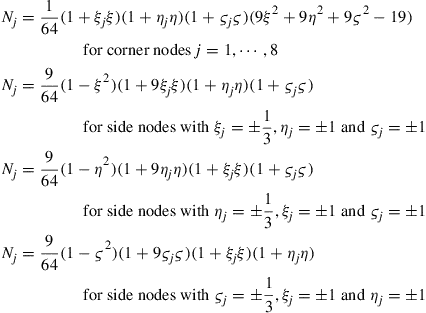
Figure 9.15a shows a 20-nodal tri-quadratic element. The element has eight corner nodes and twelve mid-side nodes. The shape functions in terms of natural coordinates for the quadratic rectangular element are given as follows:
 (9.67)
where (ξj, ηj) are the natural coordinates of node j. It is very easy to observe that the shape functions possess the delta function property. The shape function is constructed by simple inspections, making use of the shape function properties. For example, for the corner node 2 (where ξ2 = 1, η2 = −1, ζ2 = −1), the shape function N2 has to pass the following four planes as shown in Figure 9.16 to ensure it vanishes (i.e. N2 = 0) at remote nodes.
 (9.68)
The shape N2 can immediately be written as
![]() (9.69)
(9.69)
where C is a constant to be determined using the condition that it has to be unity at node 2 (ξ2 = 1, η2 = −1, ζ2 = −1), which gives
![]() (9.70)
(9.70)
We finally have
![]() (9.71)
(9.71)
which is the first equation in Eq. (9.67) for j = 2. Shape functions at all the other corner nodes can be constructed in the same manner. As for the mid-side nodes, say node 9, we enforce the shape function passing through the following three planes as shown in Figure 9.17.
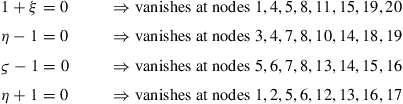 (9.72)
The shape function, N9, can then immediately be written as
![]() (9.73)
(9.73)
where C is a constant to be determined using the condition that it has to be unity at node 9 (ξ9 = ,1, η9 = 0, ζ9 = −1), which gives
![]() (9.74)
(9.74)
![]() (9.75)
(9.75)
which is the third equation in Eq. (9.67) for j = 9.

Figure 9.15 High order 3D serendipity elements. (a) 20-node quadratic element; (b) 32-node cubic element.
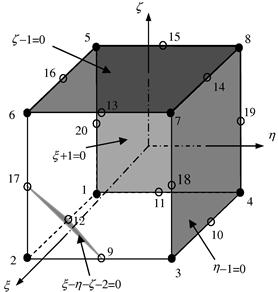
Figure 9.16 Construction of a 20-node serendipity element. Four flat planes passing through the remote nodes of node 9 are used.
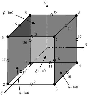
Figure 9.17 Construction of a 20-node serendipity element. Four flat planes passing through the remote nodes of node 9 are used.
Because the delta function property is used for the construction of shape functions given in Eq. (9.67), they naturally possess the delta function property. It can be easily seen that all the shape functions can be formed using the following common set of basis functions.
![]() (9.76)
(9.76)
![]()
that are linearly-independent and contains all the linear terms. From Lemma 2 and 3, we confirm that the shape functions are partitions of unity, and at least linear field reproduction. Hence, they satisfy the sufficient requirements for FEM shape functions.
Following a similar procedure, the shape functions for the 32-node tri-cubic element shown in Figure 9.15b can be written as
 (9.77)
The reader is encouraged to identify the planes that are used to form these shape functions listed in Eq. (9.77). When ζ = ζI = 1, the above equations reduce to the two dimensional serendipity quadratic and cubic element defined by Eqs. (7.113) and (7.123) respectively.
9.5 Elements with curved surfaces
Using high order elements, elements with curved surfaces can be used in the modeling. Two frequently used higher order elements of curved edges are shown in Figure 9.18a. In formulating these types of elements, the same mapping technique used for the linear quadrilateral elements (Section 9.3) can be used. In the physical coordinate system, elements with curved edges are first formed in the problem domain as shown in Figure 9.18a. These elements are then mapped to the natural coordinate system using Eq. (9.34). The elements mapped in the natural coordinate system will have straight edges as shown in Figure 9.18b.

Figure 9.18 3D solid elements with curved surfaces. (a) Elements with curved surfaces in the physical coordinate system; (b) Brick elements obtained by mapping.
Higher order elements of curved surfaces are often used for modeling curved boundaries. Note that elements with excessively curved edges may cause problems in the numerical integration. Therefore, more elements should be used where the curvature of the boundary is large. In addition, it is recommended that in the internal portion of the domain, elements with straight edges should be used whenever possible.
9.6 Case study: Stress and strain analysis of a quantum dot heterostructure
Quantum dots are clusters of atoms nanometers in size, usually made from semiconducting materials like silicon, cadmium selenide or gallium arsenide. What makes quantum dots interesting is that they have unusual electrical and optical properties, hence they have the potential for use in a wide variety of novel electronic devices, including light emitting diodes, photovoltaic cells, and quantum semiconductor lasers. An interesting way of fabricating such quantum dot structures is to actually grow the dots directly by depositing a thin film layer of material on a substrate under appropriate growth conditions. Usually, the thin film layer is of a different material with the substrate material and, thus, such structures are also known generally as heterostructures. This growth mode is due to the mismatch in the lattice parameters of the different materials and is known as the Stranski-Krastanow (SK) growth mode.
The growth of the quantum dot structures is partly driven by the strain energy in the thin film, which makes studying the stress distribution in the film a crucial part of understanding the growth mechanism. In this case study, an example of modeling a 3D finite element model to analyze the stress distribution in and around such structures will be shown. The stress distribution also affects the electrical and optical properties of the quantum dot structure.
Figure 9.19 shows a schematic representation of a quantum dot grown on top of the substrate and embedded in a cap layer. This is just a single quantum dot and can probably be considered as a single basic unit of the heterostructure. In reality, there could be many of such quantum dots distributed on top of a layer of substrate. It can also be seen from Figure 9.19 that the quantum dot is usually pyramidal or trapezoidal in shape. The pyramidal shape of the quantum dot is often approximated by many analysts by using a 2D axisymmetric model of a cone. However, it should be noted that using a 2D axisymmetric model is not fully representative of the pyramidal shape. For the purposes of this chapter, this case study will use the 3D solid element to model the structure.

9.6.1 Modeling
Meshing
As mentioned, the modeling of any 3D structure is generally more complex and tedious. In this case, 8-nodal, hexahedron elements are being used for the meshing of the 3D geometry. It can be seen from Figure 9.19 that the problem domain is very much symmetrical. Therefore, in order to work on a more manageable problem, a quarter of the model is being modeled using mirror symmetry. Note that it is also possible to use a one-eighth model, which then requires the use of multiple point constraints (MPC) equations (see Chapter 11).
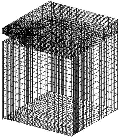
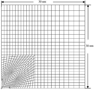
Proper meshing in this case is very important as it has been found that a poor mesh usually yields bad results. The 3D mesh of the heterostructure is shown in Figures 9.20 and 9.21. The model is generally divided into two main parts geometrically for the analysts to distinguish them more conveniently. The parts of the heterostructure comprising the substrate and the cap layer, as shown in Figure 9.19, are grouped together as the matrix; and the parts of the heterostructure comprising the wetting layer and the quantum dot itself are grouped together as the island. Figure 9.22 also shows the plan view of the mesh of the island (or matrix). It can be seen from this figure how smaller elements are concentrated at and around the pyramidal quantum dot. To generate the mesh here, the analyst has employed the aid of automatic mesh generators that can still mesh the relatively complex shape of the pyramid with hexahedron elements. Some mesh generators may not be able to achieve this and one may end up with either tetrahedron elements or a mixture of both hexahedron and tetrahedron elements.

Material properties
In this case study, the heterostructure system of indium arsenide (InAs) quantum dots embedded in gallium arsenide (GaAs) substrate and cap layer is being analyzed. Therefore, the matrix part of the model will be of the material GaAs and the island part of the model will be of the material InAs. This is an example of the convenience of dividing the model into these two parts. It is assumed here that the materials have isotropic properties and they are listed in Table 9.1.
Constraints and boundary conditions
As the model is a symmetric quarter model, symmetrical boundary conditions must be applied. Here it means that the nodes on the planes corresponding to x = 0 nm, y = 0 nm, x = 30 nm, and y = 30 nm have their displacement components normal to their respective planes constrained. Another displacement boundary condition would be the base of the matrix, whereby all the displacement components of the nodes are constrained.
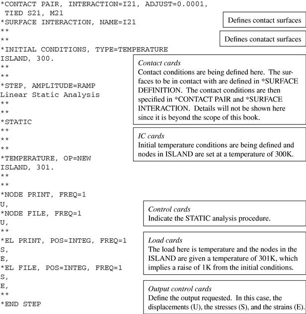
There is also a contact constraint condition imposed between the outer surfaces of the island and the surfaces of the cap layer and the substrate in the matrix. Contact modeling is a relatively advanced technique and will not be covered in this book. Basically contact modeling is used to model the sliding or the movement between two surfaces. ABAQUS offers a “tied” contact condition whereby the two surfaces in contact are actually tied to one another. This “tied” contact condition is used here to model the bonding between the island (InAs) and the matrix (GaAs).
There is actually no load acting on this model. Rather, thermal expansion is being made use of to simulate the strain induced due to the lattice mismatch between GaAs and InAs. The strain induced due to the lattice mismatch can be calculated from the lattice parameters to be −0.067. To represent this lattice mismatch, a corresponding thermal expansion coefficient of αT = 0.067 is applied to the elements in the island and the temperature is raised by 1 K. This would effectively result in an expansion of the island and because it is constrained by the matrix, thermal strain corresponding to the lattice mismatch strain is induced. Note that this thermal expansion does not take place in the physical case, but is just used to produce the mismatch strain. This thermal strain actually contributes to the force vector in the finite element equations.
9.6.2 ABAQUS input file
Parts of the ABAQUS input file for the problem defined above are shown below. As the problem is a rather large one, the full input file would consist of a large amount of data defining the nodes, elements, and so on. As such, the full data will not be included here and some parts of the input file that have been explained in previous case studies will not be explained again here.
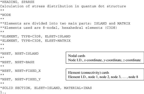

The input file would provide the information ABAQUS would need to perform tasks like forming the stiffness matrix and the force vector (no mass matrix since this is a static analysis). The full input file may consist of many pages, which is common for large problems.
9.6.3 Solution process
The information provided in the input file is very similar to previous case studies. The nodal and element connectivity information is read for the formulation of the element matrices. The element type used here is C3D8, which represents a 3D, hexahedral element with 8 nodes. More 3D element types are also available in the ABAQUS element library. The material properties provided in the input file will be used to formulate the element stiffness matrix (Eq. (9.51)) as well. Recall that the integration in the stiffness matrix is usually carried out using the Gauss integration scheme sampled in three directions and in ABAQUS, the default number of integration points per face of the hexahedral element is 4, making the total number of integration points per element 24. All the element matrices will be assembled together using the connectivity information provided. The application of the boundary conditions and the thermal strain induced by the thermal expansion is carried out by the specifications in the boundary cards and the load card. Finally, the finite element equation will be solved using the algorithm for static analysis as discussed in Chapter 6.
9.6.4 Results and discussion
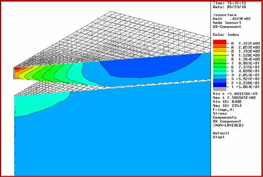
Running the problem in ABAQUS, we are able to get the stress distribution and the strain distribution as requested in the input file. Figures 9.23 and 9.24 shows the stress distribution obtained in the matrix and island, respectively, of a particular plane of θ = 45°, where θ is measured from the x–z plane counter-clockwise. Despite the extra effort in the meshing of a 3D model, the advantage of it is that it enables the analyst to view, in this case, the stress distribution in any arbitrary plane in the entire model. This would be difficult to achieve if a 2D, axisymmetric approximation was carried out instead. From the stress distribution, one would observe that there are compressive stresses in the island and tensile stresses in the matrix area above the island. In the island, there is also stress relaxation in the quantum dot with the maximum stress relaxation at the tip of the pyramidal quantum dot. This actually verifies the thermodynamics aspect of quantum dot formation, since the formation of a quantum dot results in a lower energy level (lower elastic strain energy). The tensile stress in the matrix area above the quantum dot is also important as this stress actually causes subsequent quantum dots to be formed directly above the buried quantum dot when a subsequent InAs layer is deposited.

9.7 Review questions
1. Can 3D solid elements be used for solving 2D plane stress and plane strain problems? Give a justification for your answer.
2. What is the difference between using tetrahedron elements and hexahedron elements derived using assemblage of tetrahedron elements? Can they give the same results for the same problem? Give a justification for your answer.
3. Give shape functions N1, N2, N3, and N4 for the element given in Figure 9.25.
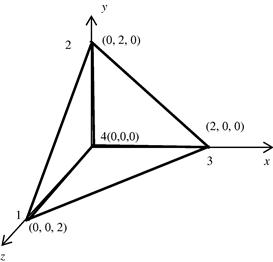
4. Evaluate the strain matrix B for the tetrahedral solid element shown in Figure 9.25.
5. For the element shown in Figure 9.25, assume the nodal displacements have been found as (in cm):

Determine the strains and then the stresses in the element. Let E = 210 GPa and ν = 0.3.
6. Can one develop pentahedron elements? How?
7. How many Gauss points should be used for evaluating mass and stiffness matrices for 4-node tetrahedron elements? Give a justification for your answer.
8. How many Gauss points should be used for evaluating mass and stiffness matrices for 8-node hexahedron elements? Give a justification for your answer.
9. If a higher order shape function is used, do Eqs. (9.30) and (9.63) still hold? Give a justification for your answer.
10. Consider a uniform, isotropic square “plate” with an in-plane dimension of 1 m by 1 m. The plate is clamped on all edges (CCCC), made of a material with Young’s modulus E = 70 GPa and Poisson ratio υ = 0.3. Using 3D block element with a density of 16 × 16 in the plate-plane to perform the analysis; compare the 3D FEM solution with the FEM solution using plate elements with a density of 16 × 16, and the analytical solution (based on thin plate theory) in terms of the deflection at the center of the plate. You are requested to perform the following studies:
a. The plate is of thickness 0.01 m;
b. The plate is of thickness 0.1 m;
c. The plate is of thickness 0.2 m;
d. The plate is of thickness 0.5 m.
References
1. Eisenberg MA, Malvern LE. On finite element integration in natural coordinates. Int J Num Meth Eng. 1973;7:574–575.
2. Rao SS. The Finite Element in Engineering. 3rd edition Butterworth-Heinemann 1999.
3. Washizu K, et al. Finite Elements Handbook. vols. 1 and 2 Japan: Baitukan; 1981; in Japanese.
4. Zienkiewicz OC, Taylor RL. The Finite Element Method. 5th edition Butterworth-Heinemann 2000.