Special Purpose Elements
10.1 Introduction
This chapter introduces some special purpose elements and methods that are designed for specific circumstances. They are used to either simplify meshing and calculation or to obtain better accuracy, which the usual elements cannot obtain. These include crack tip elements, infinite elements, finite strip elements, and strip elements. In addition, a brief introduction is provided on the recent meshfree and the smoothed finite element methods (S-FEMs). The characteristics of these elements and recent advanced models are summarized in Table 10.1.
Table 10.1
Special elements and recent advanced methods.
| Elements | Application | Approach/Features |
| Crack tip elements | Simulation of problem domain with the cracks | Use of mapping techniques to create singular stress field; reduce element density near crack tips |
| Infinite elements | Simulation problems with an infinite or semi-infinite domain | Use of mapping techniques to create fields that decay with distance; very few elements are needed for model infinite boundary |
| Finite strip elements | Model structures with a regular geometric domain | Shape function with series expansion in one direction; very few elements needed; simple boundary conditions |
| Strip elements | Model structures with a regular geometric domain | Semi-analytical approach; very few elements needed; arbitrary boundary conditions including infinite boundaries |
| Meshfree methods (GR Liu, 2009) | Adaptive analyses, highly non-linear problems, crack propagation, high velocity impact, penetration, and explosion | Numerical operations (interpolation, integration, etc.) can be beyond the elements, based on nodes and/or particles. They may use T-meshes (triangles for 2D, tetrahedra and triangular-prisms for 3D), but can be generated automatically for complicated geometries |
| Smoothed finite element methods or S-FEM (Liu and Trung, 2010) | Adaptive analyses, highly non-linear problems for solids and structures, crack propagation, fluid-structural interaction. Existing models are: ES-FEM; NS-FEM; CS-FEM; FS-FEM; and αFEM | Interpolation based on elements; use of smoothing operations that can be node-based, edge-based, cell-based, face-based smoothing cells or their combination. No integration is needed for the weakform. It works very well for T-meshes that can be generated automatically for complicated geometries |
10.2 Crack tip elements
In fracture mechanics, the region around the tip of the crack is usually of much interest to analysts since the tip is a singularity point where the stress level becomes mathematically infinite. When modeled with the conventional, polynomial-based finite elements discussed in previous chapters, the finite element approximations are usually not accurate around the crack tip. Refinement is a simple way to improve the solution near the crack tip, but this may not prove feasible at times and is highly inefficient when computational resources are limited. Even if the elements are refined around the crack tip, it is not possible to capture the singularity at the crack tip, by polynomial approximation. It will be a better option to model such a problem with what is known as crack tip elements, sometimes also known as singularity elements. Such an element was introduced at almost the same time by Henshell and Shaw (1975) and Barsoum (1976, 1977).
From the theory of linear elastic fracture mechanics, the stresses near the crack tip are characterized by the stress intensity factor, KI, in Mode I fracture as
 (10.1)
and the displacements near the crack tip are expressed as
 (10.2)
where G is the shear modulus, and κ = 3 − 4υ (plane strain) or (3 − υ)/(1 + υ) (plane stress). Mode I fracture is considered to be the opening of the crack as shown in Figure 10.1 with r being the radial axis originated at the crack tip and θ the polar axis. From Eqs. (10.1) and (10.2), it can be noted that the stress varies with ![]() and the displacements vary proportionally with
and the displacements vary proportionally with ![]() . Note the presence of singularity of the stresses at the crack tip when r approaches zero.
. Note the presence of singularity of the stresses at the crack tip when r approaches zero.

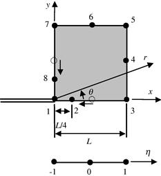
To approximate the behavior of the singular stresses and ![]() displacements near the crack tip predicated by the theory of fracture mechanics, a special 8-nodal, quadratic, isoparametric element can be formulated, as shown in Figure 10.2. This element is exactly the same as the usual 8-nodal isoparametric quadratic element, except that the middle nodes on the edges to the crack tip are moved by a quarter of the edge-length towards the crack tip. The following explains how the stress singularity is created by this simple modification.
displacements near the crack tip predicated by the theory of fracture mechanics, a special 8-nodal, quadratic, isoparametric element can be formulated, as shown in Figure 10.2. This element is exactly the same as the usual 8-nodal isoparametric quadratic element, except that the middle nodes on the edges to the crack tip are moved by a quarter of the edge-length towards the crack tip. The following explains how the stress singularity is created by this simple modification.

Consider the element edge joining nodes 1, 2, and 3 of the isoparametric quadratic element shown in Figure 10.3, with node 1 at the crack tip. Following the formulation of the conventional isoparametric 8-nodal element, the coordinate x and the displacement u are both interpolated by shape functions as follows:
![]() (10.3)
(10.3)
![]() (10.4)
(10.4)
Let both x and u be measured from node 1, and let the mid-edge node 2 be moved to the quarter-point node 2. For an edge of length L, we have
![]() (10.5)
(10.5)
Substitution of Eq. (10.5) into Eqs. (10.3) and (10.4) leads to
![]() (10.6)
(10.6)
![]() (10.7)
(10.7)
Simplifying the above equations will give us
![]() (10.8)
(10.8)
![]() (10.9)
(10.9)
Now, we know that along the x axis, x = r. Therefore,
![]() (10.10)
(10.10)
Substitution of Eq. (10.10) into Eq. (10.9) leads to
![]() (10.11)
(10.11)
Notice that by shifting the middle node to the quarter position, the displacement now follows a behavior that is proportional to ![]() . Furthermore, the strain relates directly to derivatives of the displacement:
. Furthermore, the strain relates directly to derivatives of the displacement:
![]() (10.12)
(10.12)
where from Eqs. (10.8) and (10.10),
![]() (10.13)
(10.13)
Thus, by using Eqs. (10.9), (10.12), and (10.13),
![]() (10.14)
(10.14)
It is noted that the strain will have a behavior given by Eq. (10.14): proportional to ![]() . Since the stress is proportional to the strain, this is also true for the stresses. Therefore it can be seen that by shifting the middle node 2 to the quarter position, we are able to obtain an approximation that follows the behavior of the stresses and displacements near the crack tip as predicted by linear fracture mechanics. Similar procedures can be applied to the other side consisting of nodes 1, 7, and 8.
. Since the stress is proportional to the strain, this is also true for the stresses. Therefore it can be seen that by shifting the middle node 2 to the quarter position, we are able to obtain an approximation that follows the behavior of the stresses and displacements near the crack tip as predicted by linear fracture mechanics. Similar procedures can be applied to the other side consisting of nodes 1, 7, and 8.
By the same argument, other types of crack tip elements with different shapes can also be obtained and some examples are shown in Figure 10.4.

10.3 Methods for infinite domains
There are many problems in real life that actually involve an infinite or semi-infinite domain, for example, the radiation of heat from a point source into space, the propagation of waves on the surface of the ground and under the ocean, and so on. For the above problems, the strength of the heat radiation and the amplitude of the waves vanish at infinity. So far, the finite element methods we have discussed in this book all include finite enclosed boundaries. If these conventional elements are used to model an infinite domain, the boundary will affect the results obtained. For the propagation of waves, any finite boundary will reflect the waves and this will result in the superposition of the transmitted and reflected waves. Similarly for other problems, the approximations using the conventional finite elements will thus be inaccurate. Intuitively, one might think that one solution to modeling the infinite or semi-infinite domain is to place the finite boundary far away from the area of interest. The question of “how far” will be far enough will then arise and, besides, this method would usually require excessively large numbers of elements to model regions that the analyst has little interest in. To overcome such difficulties caused by infinite or semi-infinite domains, many methods have been proposed, one of the most effective and efficient of which is the use of infinite elements.
10.3.1 Infinite elements formulated by mapping
An infinite element is created by using shape functions to approximate a sequence of decaying terms
![]() (10.15)
(10.15)
where Ci are arbitrary constants and r is the radial distance from the origin or pole, which is usually the “central” point of the problem with the infinite domain. Consider the 1D mapping of the line OPQ, which coincides with the x axis, as shown in Figure 10.5. Like the finite element formulation for isoparametric elements, the coordinates are interpolated from the nodal coordinates and thus let us propose that
![]() (10.16)
(10.16)
From Eq. (10.16), it is observed that ξ = 0 corresponds to x = xQ, ξ = 1 corresponds to x = α, and ξ = −1 corresponds to ![]() . As mentioned, r is the distance measured from the origin or pole and we assume that the pole is at O. Therefore,
. As mentioned, r is the distance measured from the origin or pole and we assume that the pole is at O. Therefore,
![]() (10.17)
(10.17)
Solving Eq. (10.16) for ξ would give
![]() (10.18)
(10.18)
If the unknown variable, say the displacement u, is approximated by a polynomial function such as
![]() (10.19)
(10.19)
Then, substituting Eq. (10.18) into (10.19) would give us a series of decaying terms in the form of Eq. (10.15) with the linear shape function in ξ corresponding to 1/r terms, quadratic to 1/r2, and so on.
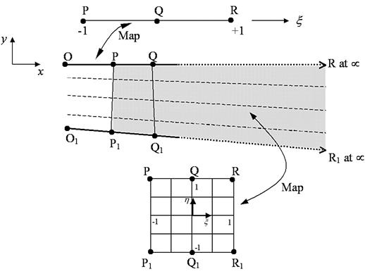
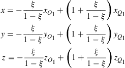
A generalization to 2D or 3D can be achieved by simple products of the 1D, infinite, mapping shown above with a standard type of shape function in η (and ζ for 3D) direction in the manner shown in Figure 10.5. First, we generalize the interpolation of Eq. (10.16) for any straight line in the x, y, and z space:
 (10.20)
Then we complete the interpolation and map the whole domain of ξη(ζ) by adding a standard interpolation in the η(ζ) directions. Thus, for element PP1QQ1RR1 in Figure 10.5, we can write
![]() (10.21)
(10.21)
with
![]() (10.22)
(10.22)
and map the points as shown. In a similar manner, quadratic interpolations could be used as well. These infinite elements can be joined to a standard finite element mesh as shown in Figure 10.6.

10.3.2 Gradual damping elements
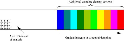
Using elements with gradually increased artificial damping elements attached on the regular finite element mesh is a very efficient way to model vibration and wave propagation problems with infinite boundaries. This method was proposed by Liu (1994) and Liu and Quek (2003) for modeling such problems using discrete numerical methods. One of the applications of this technique is in the study of lamb wave propagation in infinite plates or beams. Lamb waves are dispersive waves that involve multiple characteristic reflections with the top and bottom surface of the plate as it progresses along the plate as shown schematically in Figure 10.7. This method uses the conventional finite elements and the infinite domain is approximated by adding additional elements with a gradual increase in damping to damp down the amplitude of the propagating waves, as shown in Figure 10.8. A detailed analysis of the method was given by Liu (1994) and Liu and Quek (2003).

10.3.3 Coupling of FEM and the boundary element method
Another effective method of dealing with infinite domains is to use the FEM coupled with the boundary element method (BEM). The FEM is used in the interior portions of the problem domain where the problem is very complex (non-linear, inhomogeneous, etc), and BEM is used for exterior portion that can extend to infinity. Much research has been done in this area. An example can be found in a paper by Liu et al. (1992) for wave propagation problems.
10.3.4 Coupling of FEM and the strip element method
Coupling of FEM with the strip element method (SEM; see Section 10.5) can also effectively handle infinite domains. In such a combination, the FEM is used in the interior portions of the problem domain where the problem is very complex (anisotropy, non-linear, inhomogeneous, complex geometry, etc), and SEM is used for exterior portions that can extend to infinity. This combination is applicable for domains of anisotropic materials (see Liu, 2002).
10.4 Finite strip elements
Using finite strip elements, instead of the conventional finite elements, can be a very effective method for solving structural problems involving regular geometry and simple boundary conditions, as shown in Figure 10.9. This method was developed by Y. K. Cheung in 1968. In his method, the structure is divided into 2D strips or 3D prisms or layers of sub-domains. This method usually requires the geometry of the structure to be constant along one or two coordinate axes so that the width of the strip or the cross-section of the prism or layer will not change from one end to the other.

10.5 Strip element method
The strip element method (SEM) was proposed by Kausel and Roësset (1977) and Tassoulas and Kausel (1983) for solids of isotropic materials, and Liu and co-workers (Liu and Achenbach, 1994; Liu and Achenbach, 1995; Liu and Xi, 2001) for solids of anisotropic materials. The SEM is a semi-analytic method for stress analysis of solids and structures. It has been mainly applied for solving wave propagating in composite laminates. The SEM is a semi-exact method that discretizes the problem domain in one or two directions. Polynomial shape functions are then used in these directions together with the weak forms of system equation to produce a set of dimension-reduced spatial differential equations. These differential equations are then solved analytically. The dimension of the final discretized system equations would therefore be reduced by one order. The details can be found in a monograph by Liu and Xi (2001). Due to the semi-analytic nature of the SEM, it is applicable for problems of arbitrary boundary conditions including the infinite boundary conditions.
The coupling of SEM with FEM has also been proposed by Liu (2002). In such a combination, the FEM is used for small domains of complex geometry and SEM is used for bulky domains of regular geometry.
10.6 Meshfree methods
The FEM uses elements, and all the numerical operations are based on elements, strictly following the Galerkin weakform or the standard variational/energy principles. The FEM has dominated the area of numerical methods during the last half a century. However, shortcomings for the FEM are also becoming evident. We have seen that the FEM model is a stiff model, meaning that it behaves stiffer than the actual real solids/structures. We have also found that FEM models using T-meshes (triangles for 2D and tetrahedron for 3D) are particularity stiff, and the stress solutions are often inaccurate. However, we engineers prefer to use such a simple T-mesh, because it can be generated automatically for complicated geometries, which is extremely important for automation in computations. It is believed that automation is the future in computer modeling and simulation. Therefore, efforts have been made in improving the FEM, which led to the development of a class of methods called meshfree methods in the past few decades (Liu, 2009).
In meshfree methods, numerical operations (interpolation, integration, etc.) are conducted beyond the elements and based on nodes and/or particles. Some meshfree methods, such as the smoothed particle hydrodynamics (SPH) (Liu and Liu, 2003), use only particles. The SPH method is powerful enough to simulate highly dynamic problems, including high velocity impact, penetration, and explosions. Some meshfree methods, such as the Smoothed Point Interpolation Methods (S-PIM) and the Element Free Galerkin (EFG) methods can use T-meshes (triangles for 2D and tetrahedra for 3D), and therefore are good candidates for adaptive analyses, highly non-linear problems, and crack propagation problems. The formulation of S-PIM is based on smoothing the weakened weak (W2) form, and that of EFG is still based on the Galerkin weakform. Details on this new development can be found in Meshfree Methods: Moving Beyond the Finite Element Method, by Liu (2009), where major meshfree methods are introduced in great detail.
10.7 S-FEM
The meshfree method can be computationally more expensive compared to the well-established FEM. The idea of combining the meshfree techniques with the FEM therefore seems like an attractive proposition. This has led to the recent development of the S-FEM that combines the existing standard FEM and the existing strain smoothing techniques used in meshfree methods (Liu and Trung, 2010). In S-FEM, the field function interpolation is based on elements (as in the FEM), but it uses smoothed strains to construct numerical models, and hence no integration is needed for the weakform. The formulation of S-FEM can be based either on smoothed weakform or the W2 form. The key to the S-FEM lies in how one performs the strain operations. The currently proven strain smoothing operations are based on node-based, edge-based, cell-based, and face-based smoothing domains, or even their combinations. Therefore, there is a family of models called ES-FEM; NS-FEM; CS-FEM; FS-FEM; and αFEM. Figure 10.10 shows an ES-FEM for 2D problems and an FS-FEM for 3D problems. It works very well for T-meshes that can be generated automatically for complicated geometries.

Figure 10.10 Smoothing domains used in S-FEM for 2D and 3D problems. Left: edge-based smoothing domains in 2D problems; Right: face-based smoothing domains for 3D problems.
The S-FEM has been found to have the following significant features: (1) S-FEM models are always “softer” than the standard FEM, promising to provide more effective numerical solutions; (2) S-FEM models give more freedom and convenience in constructing shape functions for special purposes or enrichments (e.g., various degrees of singular fields near the crack tip, highly oscillating fields, etc.); (3) S-FEM models allow the use of distorted elements and general n-sided polygonal elements; (4) NS-FEM offers a much simpler tool to estimate the quality of the solution (global error, bounds of solutions, etc) for many types of problems; (5) the αFEM, a combination of various S-FEM models, can offer solutions of very high accuracy. Interested readers are referred to the S-FEM book by Liu and Trung (2010).
References
1. Henshell RD, Shaw KG. Crack tip elements are unnecessary. Int J Num Meth Eng. 1975;9:495–509.
2. Barsoum RS. On the use of isoparametric finite elements in linear fracture mechanics. International Journal for Numerical Methods in Engineering. 1976;10:25–38.
3. Barsoum RS. Triangular quarter point elements as elastic and perfectly elastic crack tip elements. International Journal for Numerical Methods in Engineering. 1977;11:85–98.
4. Liu GR. A combined finite element/strip element method for analyzing elastic wave scattering by cracks and inclusions in laminates. Computational Mechanics. 2002;28:76–81.
5. Kausel E, Roësset JM. Semianalytic hyperelement for layered strata. Journal of the Engineering Mechanics Division. 1977;103(4):569.
6. Tassoulas JL, Kausel E. Elements for the numerical analysis of wave motion in layered strata. Int J Numer Methods Eng. 1983;19:1005–1032.
7. Liu GR, Xi ZC. Elastic Waves in Anisotropic Laminates. CRC Press 2001.
8. Liu GR. Meshfree Methods: Moving Beyond the Finite Element ethod. 2nd ed. Boca Raton: CRC Press; 2009.
9. Liu GR, Achenbach JD. A strip element method for stress analysis of anisotropic linearly elastic solids. ASME Journal of Applied Mechanics. 1994;61:270–277.
10. Liu GR, Achenbach JD. A strip element method to analyze wave scattering by cracks in anisotropic laminated plates. ASME Journal of Applied Mechanics. 1995;62:607–613.
11. Liu GR, Quek SS. A non-reflecting boundary for analyzing wave propagation using the finite element method. Finite Elements in Analysis and Design. 2003;39(5):403–417.
12. Liu GR, Liu MB. Smoothed Particle Hydrodynamics: A Meshfree Particle Method. World Scientific Publishing Company 2003.
13. Liu GR, Trung Nguyen Thoi. Smoothed Finite Element Methods. Boca Raton: CRC Press; 2010.
14. Liu GR, Achenbach JD, Kim JO, Li ZL. A combined finite element method/boundary element method for V(z) curves of anisotropic-layer/substrate configurations. Journal of the Acoustical Society of America. 1992;92(5):2734–2740.