FEM for Trusses
4.1 Introduction
A truss is one of the simplest and most widely used structural members. It is a straight bar that is designed to take only axial forces, and therefore deforms only along its axial direction. An example of a structure consisting of an assemblage of trusses can be seen in Figure 2.7. The cross-section of the truss can be arbitrary, but the dimensions of the cross-section should be much smaller than that in the axial direction—a characteristic of a truss or bar structure.
Finite element equations for such truss members will be developed in this chapter. The one-dimensional element developed is commonly known as the truss element or bar element. Such elements are applicable for analysis of skeletal-type truss structural systems both in two-dimensional planes and in three-dimensional space. The basic concepts, procedures, and formulations can also be found in many existing textbooks (see, e.g. Reddy, 1993; Rao, 1999; Zienkiewicz and Taylor, 2000).
In planar trusses there are two components in the x and y directions for the displacements as well as for the forces. For spatial trusses, however, there will be three components in the x, y, and z directions for both displacements and forces. In skeletal structures consisting of truss members, the truss members are joined together by pins or hinges (as opposed to welding), so that only forces (not moments) are transmitted between the bars. For the purpose of explaining the concepts more clearly, this book will assume that the truss elements have a uniform cross-section. The concepts described will apply equally and easily to the formulation of bars with varying cross-sections. Note, however, that there is no reason from a mechanics viewpoint to use bars with a varying cross-section, because the force in a bar is uniform.
4.2 FEM equations
4.2.1 Shape function construction
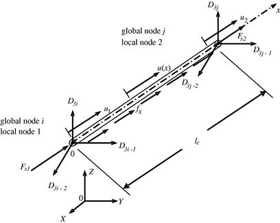
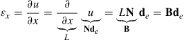
Consider a structure consisting of a number of trusses or bar members. Each of the members can be considered as a truss/bar element of a uniform cross-section bounded by two nodes (nd= 2). Consider a bar element with nodes 1 and 2 at each end of the element, as shown in Figure 4.1. The length of the element is le. The local x axis is taken in the axial direction of the element with the origin at node 1. In the local coordinate system, there is only one DOF at each node of the element, and that is the axial displacement. Therefore, there is a total of two DOFs for the element, i.e. ne = 2. In the FEM discussed in the previous chapter, the displacement in an element should be written in the form
![]() (4.1)
(4.1)
where uh is the approximation of the axial displacement within the element, N is a matrix of shape functions that possess the properties described in Chapter 3, and de should be the vector of the displacements at the two nodes of the element:
 (4.2)
(4.2)
The question now is how we can determine the shape functions for the truss element.
We can follow the standard procedure described in Section 3.4.3 for constructing shape functions, and assume that the axial displacement in the truss element can be given in a general form
 (4.3)
(4.3)
where uh is the approximation of the displacement, α is the vector of two unknown constants, α0 and α1, and p is the vector of polynomial basis functions (or monomials). Since we have two nodes with a total of two DOFs in the element, we choose to have two terms of basis functions as in Eq. (4.3). Notice that we choose to use matrix expression in Eq. (4.3), despite the simplicity of the equation. This is to intentionally help readers get familiar with matrix expression and manipulation, which is essential in FEM formulations. For this particular problem, the polynomial basis functions consist of terms up to the first order. Depending upon the problem, we could use higher order polynomial basis functions. The order of polynomial basis functions up to the nth order can be given by
![]() (4.4)
(4.4)
In this case, vector α shall have n unknown constants, α0, α1, … αn, and Eq. (4.3) can still be written as,
![]() (4.3a)
(4.3a)
The number of terms of basis functions or monomials we should use depends upon the number of nodes and degrees of freedom in the element.
Note that we usually use polynomial basis functions of complete orders, meaning we do not skip any lower terms in constructing Eq. (4.3a). This is to ensure that the shape functions constructed will be able to reproduce complete polynomials up to an order of n. If a polynomial basis of the kth order is skipped, the shape function constructed will only be able to ensure a consistency of (k – 1)th order, regardless of how many higher orders of monomials are included in the basis. This is because of the consistency property of the shape function (Property 1), discussed in Section 3.4.4. From Properties 3, 4, and 5 discussed in Chapter 3, we can expect that the complete linear basis functions used in Eq. (4.3) guarantee that the shape function to be constructed satisfies the sufficient requirements for the FEM shape functions: the delta function property, partition of unity, and linear field reproduction.
In deriving the shape function, we use the fact that
![]() (4.5)
(4.5)
Using Eqs. (4.3) and (4.5), we then have
 (4.6)
(4.6)
For le > 0, the moment matrixP is clearly not singular. Thus, solving the above equation for α, we have
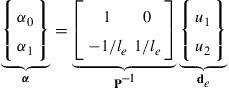 (4.7)
(4.7)
Substituting the above equation back into Eq. (4.3), we obtain
 (4.8)
(4.8)
which is in the form of Eq. (4.1). The matrix of shape functions is then obtained in the form
![]() (4.9)
(4.9)
where the shape functions for a truss element can be finally written as
 (4.10)
Notice that we obtained two shape functions because we have two DOFs in the truss elements.
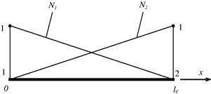
It is easy to verify that these two shape functions satisfy the delta function property defined by Eq. (3.34), and the partitions of unity in Eq. (3.41). We leave this verification to the reader as a simple exercise. The graphical representation of the linear shape functions is shown in Figure 4.2. It is clearly shown that Ni gives the shape of the contribution from nodal displacement at node i, and that is why it is called a shape function. In this case, the shape functions vary linearly across the element, and they are termed linear shape functions. Substituting Eqs. (4.9), (4.10), and (4.2) into Eq. (4.1), we have
![]() (4.11)
(4.11)
which clearly states that the displacement within the element varies linearly for any given nodal displacements u1 and u2. The element is therefore called a linear element.
4.2.2 Strain matrix
As discussed in Chapter 2, there is only one stress component σx in a truss, and the corresponding strain can be obtained by
![]() (4.12)
(4.12)
which is a direct result from differentiating Eq. (4.11) with respect to x. Note that the strain in Eq. (4.12) is a constant value (does not vary with x) in the element for any given nodal displacements u1 and u2.
It was mentioned in the previous chapter that we would need to first obtain the strain matrix, B, after which we can obtain the stiffness and mass matrices. In this two-node element case, this can be easily done. Equation (4.12) can be re-written in a matrix form as
 (4.13)
where the strain matrix B has the following form for the truss element:
![]() (4.14)
(4.14)
4.2.3 Element matrices in the local coordinate system
Once the strain matrix B has been obtained, the stiffness matrix for truss elements can be obtained using Eq. (3.71) from the previous chapter:
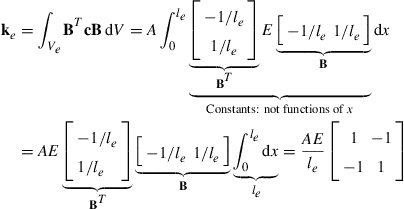 (4.15)
where A is the area of the cross-section of the truss element. Note that the material constant matrix c reduces to the elastic modulus, E, for the one-dimensional truss element (see Eq. (2.39)). It is noted that the element stiffness matrix as shown in Eq. (4.15) is symmetrical. This confirms the proof given in Eq. (3.73). Making use of the symmetry of the stiffness matrix, only half of the terms in the matrix need to be evaluated and stored during computation.
The mass matrix for truss elements can be obtained using Eq. (3.75):
 (4.16)
Similarly, the mass matrix is found to be symmetrical.
The nodal force vector for truss elements comprises contributions from the body force and the surface force and can be obtained using Eqs. (3.78), (3.79), and (3.81). Suppose, as an example, the element is loaded by an evenly distributed force fx (N/m) along the x axis, and two concentrated forces Fs1 (N) and Fs2 (N), respectively, at two nodes, 1 and 2, as shown in Figure 4.1. Note that for a 1D truss element, a force distributed along the length of the truss is considered a body force (like for example, the self weight of the truss if that is to be taken into consideration). On the other hand, surface forces are the forces applied to the end nodes. The total nodal force vector can therefore be written as
 (4.17)
Notice that an evenly distributed force acting along the length of the truss element contributes equally at the two nodes, as shown in Eq. (4.17). Note also that the “surface” force for our 1D problem is just the two concentrated point forces at the endpoints of the bar.
4.2.4 Element matrices in the global coordinate system
Element matrices in Eqs. (4.15), (4.16), and (4.17) were formulated based on the local coordinate system, where the x axis coincides with the mid axis of the bar 1–2, shown in Figure 4.1. In a typical assemblage of trusses, there are many bars of different orientations and at different locations. To assemble all the element matrices to form the global system matrices, a coordinate transformation has to be performed for each element to formulate its element matrix based on the global coordinate system for the entire truss structure. The following performs the transformation for both spatial and planar trusses.
4.2.4.1 Spatial trusses
Assume that the local nodes 1 and 2 of the element correspond to the global nodes i and j, respectively, as shown in Figure 4.1. The displacement at a global node in space should have three components in the X, Y, and Z directions, and numbered sequentially. For example, the three components at the ith node are denoted by D3i–2, D3i–1, and D3i. The coordinate transformation gives the relationship between the displacement vector de based on the local coordinate system and the displacement vector De for the same element, but based on the global coordinate system XYZ:
![]() (4.18)
(4.18)
where
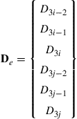 (4.19)
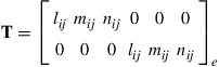
and T is the transformation matrix for the truss element, given by
 (4.20)
in which
 (4.21)
are the direction cosines of the axial axis of the element, which are the projections of the local axial axis onto the global X, Y, and Z axes. It is easy to confirm that
![]() (4.22)
(4.22)
where I is an identity matrix of 2 × 2. Therefore, matrix T is an orthogonal matrix. The length of the element, le, can be calculated using the global coordinates of the two nodes of the element by
![]() (4.23)
(4.23)
Equation (4.18) can be easily verified, as it simply says that at node i, d1 equals the summation of all the projections of D3i–2, D3i–1, and D3i onto the local x axis, and the same can be said for node j. The matrix T for a truss element transforms a 6 × 1 vector in the global coordinate system into a 2 × 1 vector in the local coordinate system.
The transformation matrix also applies to the force vectors between the local and global coordinate systems:
![]() (4.24)
(4.24)
where
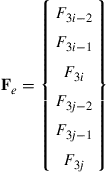 (4.25)
in which F3i−2, F3i−1, and F3i represent the three components of the force vector at node i based on the global coordinate system.
Substitution of Eq. (4.18) into Eq. (3.89) leads to the element equation based on the global coordinate system:
![]() (4.26)
(4.26)
Pre-multiply TT to both sides in the above equation to obtain:
![]() (4.27)
(4.27)
or
![]() (4.28)
(4.28)
where
 (4.29)
and
 (4.30)
Note that the coordinate transformation preserves the symmetrical properties of both stiffness and mass matrices.
For the corresponding transformation of the force vector given in Eq. (4.17), we obtain
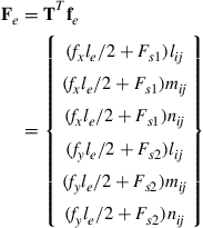 (4.31)
Note that the element stiffness matrix Ke and mass matrix Me have a dimension of 6 × 6 in the three-dimensional global coordinate system, and the displacement De and the force vector Fe have a dimension of 6 × 1.
4.2.4.2 Planar trusses
For a planar truss, the global coordinates X–Y can be employed to represent the plane of the truss. All the formulations of coordinate transformation can be obtained from that for the spatial trusses counterpart by simply removing the rows and/or columns corresponding to the z- (or Z-) axis. The displacement at the global node i should have two components in the X and Y directions only: D2i−1 and D2i. The coordinate transformation, which gives the relationship between the displacement vector de based on the local coordinate system and the displacement vector De, has the same form as Eq. (4.18), except that
 (4.32)
and the transformation matrix T is given by
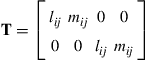 (4.33)
The force vector in the global coordinate system is
 (4.34)
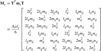
All the other equations for a planar truss have the same form as the corresponding equations for a spatial truss. The Ke and Me for the planar truss have a dimension of 4 × 4 in the global coordinate system. They are listed as follows:
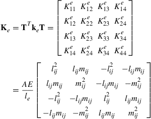 (4.35)
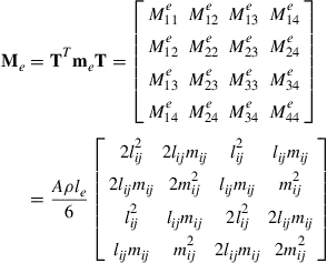 (4.36)
4.2.5 Boundary conditions
The stiffness matrix Ke in Eq. (4.28) is usually singular, because the whole structure can perform rigid body movements. There are two DOFs of rigid movements for planer trusses and three DOFs for space trusses. These rigid body movements are constrained by supports or displacement constraints. In practice, truss structures are fixed somehow to the ground or to a fixed main structure at a number of the nodes. When a node is fixed, the displacement at the node must be zero, while the structure takes external loadings. This fixed displacement boundary condition can be imposed on Eq. (4.28). The imposition leads to a cancelation of the corresponding rows and columns in the stiffness matrix. The reduced stiffness matrix becomes Symmetric Positive Definite (SPD), if sufficient displacements are constrained to remove all the possible rigid movements.
4.2.6 Recovering stress and strain
Equation (4.28) can be solved using standard routines and the displacements at all the nodes can be obtained after imposing sufficient boundary conditions. The displacements at any position other than the nodal positions can also be obtained by interpolation using the shape functions. The stress in a truss element can then be recovered using the following equation:
![]() (4.37)
(4.37)
In deriving the above equation, Hooke’s law in the form of σ = Eε is used, together with Eqs. (4.13) and (4.18).
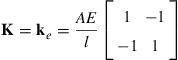
4.3 Worked examples
Exact solution
From Example 2.1, we have the exact solutions for the stress and displacements as,
![]() (4.38)
(4.38)
FEM solution
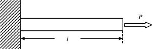
Using one element, the bar is modeled as shown in Figure 4.4. From Eq. (4.15), the stiffness matrix of the bars is given by

In this case, coordinate transformation is not required since both local and global coordinates are the same. There is also no need to perform assembly, because only one element is used. The finite element equation becomes
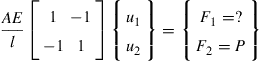 (4.39)
where F1 is the reaction force applied at node 1, which is unknown at this stage. Instead, what we do know is the displacement boundary is condition at node 1:
![]() (4.40)
(4.40)
We can then simply remove the first equation in Eq. (4.39), i.e.
![]() (4.41)
(4.41)
which leads to
![]() (4.42)
(4.42)
This is the finite element solution of the bar, which is exactly the same as the exact solution obtained in Eq. (4.38). The distribution of the displacement in the bar can be obtained by substituting Eqs. (4.40) and (4.42) into Eq. (4.1),
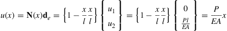 (4.43)
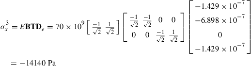
which gives the same solution as the exact solution obtained in Eq. (4.38). Using Eqs. (4.37) and (4.14), we obtain the stress in the bar
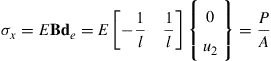 (4.44)
which is again the exact solution given in Eq. (4.38).
4.3.1 Properties of the FEM
4.3.1.1 Reproduction property of the FEM
Using the FEM, one can usually expect only an approximated solution. In Example 4.1, however, we obtained the exact solution. Why? This is because the exact solution of the deformation for the bar is a first order polynomial (see Eq. (4.38)). The shape functions used in our FEM analysis are also first order polynomials that are constructed using complete monomials up to the first order. Therefore, the exact solution of the problem is included in the set of assumed displacements in FEM shape functions. In Chapter 3, we understand that the FEM based on Hamilton’s principle guarantees to choose the best possible solution that can be produced by the shape functions. In Example 4.1, the best possible solution that can be produced by the shape function is the exact solution, due to the reproduction property of the shape functions, and the FEM has indeed reproduced it exactly. We therefore verified the reproduction property of the FEM that if the exact solution can be formed by the basis functions used to construct the FEM shape function, the FEM will always produce the exact solution, provided there is no numerical error involved in computation of the FEM solution.
Making use of this property, one may try to deliberately include additional basis functions that form the exact solution or part of the exact solution, if that is possible, so as to achieve better accuracy in the FEM solution. This technique is known as enrichment and is frequently used in simulating singular stress fields (e.g., Chapter 10 in Liu and Nguyen, 2010).
4.3.1.2 Convergence property of the FEM
For complex problems in general, the exact or analytical solution (if it exists) cannot be written in the form of a combination of monomials. Therefore, the FEM using polynomial shape functions will not be able to produce the exact solution for such a problem. The question now is, how can one ensure that the FEM can produce a good approximation of the solution for a complex problem? The insurance is given by the convergence property of the FEM, which states that the FEM solution will converge to the exact solution that is continuous at arbitrary accuracy when the element size becomes infinitely small, and as long as the complete linear polynomial basis is included in the basis to form the FEM shape functions. The theoretical background for this convergence feature of the FEM is due to the fact that any continuous function can always be approximated by a first order polynomial with a second order refinement error. This fact can be revealed by using the local Taylor expansion, based on which a continuous (displacement) function u(x) can always be approximated using the following equation:
![]() (4.45)
(4.45)
where h is the characteristic size that relates to (x – xi), or the size of the element.
According to Eq. (4.45), one may argue that the use of a constant can also reproduce the function u, but with an accuracy of O(h1). However, the constant displacements produced by the elements will not be continuous in between elements, unless the entire displacement field is constant (rigid movement), which is trivial. Therefore, to guarantee the convergence of a continuous solution, a complete polynomial up to at least the first order is used.
4.3.1.3 Rate of convergence of FEM results
The Taylor expansion up to the order of p can be given as
 (4.46)
If the complete polynomials up to the pth order are used for constructing the shape functions, the first (p + 1) terms in Eq. (4.46) will be reproduced by the FEM shape function. The error is of the order of O(hp+1); the order of the rate of convergence is therefore O(hp+1). For linear elements we have p = 1, and the order of the rate of convergence for the displacement is therefore O(h2). This implies that if the element size is halved, the error of the results in displacement will be reduced to one quarter: known as quadratic convergence.
These properties of the FEM, reproduction and convergence, are key for the FEM to provide reliable numerical results for mechanics problems, because we are assured as to what kind of results we are going to get. For simple problems whose exact solutions are of polynomial types, the FEM is capable of reproducing the exact solution using a minimum number of elements, as long as complete order of basis functions up to the order of the exact solution is used. In Example 4.1, one element of first order is sufficient. For complex problems whose exact solution is of a very high order of polynomial type, or often a non-polynomial type, it is then up to the analyst to use a proper density of the element mesh to obtain FEM results of desired accuracy where the error converges at the rate of hp+1 for the displacements.
As an extension of this discussion, we would like to introduce the concepts of so-called h-adaptivity and p-adaptivity that are intensively used in the recent development of FEM analyses. We conventionally use h to present the characteristic size of the elements, and p to represent the order of the polynomial basis functions. h-adaptive analysis uses finer element meshes (reducing h), and p-adaptivity analysis uses a higher order of shape functions (increasing p) to achieve the desired accuracy of FEM results.
Example 4.2
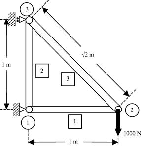
A triangular truss structure subjected to a vertical force
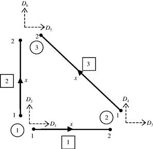
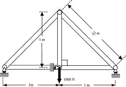
Consider the plane truss structure shown in Figure 4.5. The structure is made of three planar truss members as shown, and a vertical downward force of 1000 N is applied at node 2. The figure also shows the numbering of the elements used (in squared numbers), as well as the numbering of the nodes (in circled numbers).
The local coordinates of the three truss elements are shown in Figure 4.6. The figure also shows the numbering of the global degrees of freedom, D1, D2, …, D6, corresponding to the three nodes in the structure. Note that there are six global degrees of freedom altogether, with each node having two degrees of freedom of displacement in the X and Y directions. However, there is actually only one degree of freedom in each node in the local coordinate system for each element. From the figure, it is shown clearly that the degrees of freedom at each node have contributions from more than one element. For example, at node 1, the global degrees of freedom D1 and D2 have a contribution from elements 1 and 2. These will play an important role in the assembly of the final finite element matrices. Table 4.1 shows the dimensions and material properties of the truss members in the structure. Calculate the displacements at nodes 2 and 3, as well as the axial stresses in the three truss members.

Step 1: Obtaining the direction cosines of the elements
Knowing the coordinates of the nodes in the global coordinate system, the first step would be to take into account the orientation of the elements with respect to the global coordinate system. This can be done by computing the direction cosines using Eq. (4.21). Since this problem is a planar problem, there is no need to compute nij. The coordinates of all the nodes and the direction cosines of lij and mij are shown in Table 4.2.

Step 2: Calculation of element matrices in the global coordinate system
After obtaining the direction cosines, the element matrices in the global coordinate system can be obtained. Note that the problem here is a static one, hence there is no need to compute the element mass matrices. What is required is only the stiffness matrix. Recall that the element stiffness matrix in the local coordinate system is a 2 × 2 matrix, since the degrees of freedom are two for each element. However, in the transformation to the global coordinate system, the degrees of freedom for each element become four, therefore the element stiffness matrix in the global coordinate system is a 4 × 4 matrix. The stiffness matrices can be computed using Eq. (4.35), as is shown below:
 (4.47)
 (4.48)
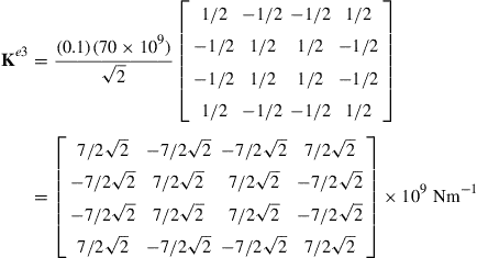 (4.49)
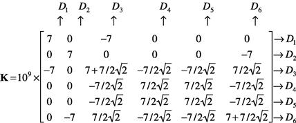
Step 3: Assembly of global FE matrices
The next step after getting the element matrices will be to assemble the element matrices into a global matrix. Since the total global degrees of freedom in the structure are six, the global stiffness matrix will be a 6 × 6 matrix. The assembly is done by adding up the contributions for each node by the elements that share the node. For example, looking at Figure 4.6, element 1 contributes to the degrees of freedom D1 and D2 at node 1, and also to the degrees of freedom D3 and D4 at node 2. On the other hand, element 2 also contributes to degrees of freedom D1 and D2 at node 1, and also to D5 and D6 at node 3. By adding the contributions from the individual element matrices into the respective positions in the global matrix according the contributions to the degrees of freedom, the global matrix can be obtained. This assembly process is termed direct assembly.
At the beginning of the assembly, the entire global stiffness matrix is zeroed initially. By adding the element matrix for element ![]() into the global element, we have
into the global element, we have
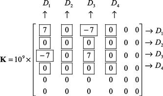 (4.50)
Note that element 1 contributes to DOFs of D1 to D4. By adding the element matrix for element 2 on top of the new global element, it becomes
 (4.51)
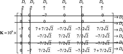
Element ![]() contributes to DOFs of D1, D2, D5, and D6. Finally, by adding the element matrix for element
contributes to DOFs of D1, D2, D5, and D6. Finally, by adding the element matrix for element ![]() on top of the current global element, we obtain
on top of the current global element, we obtain
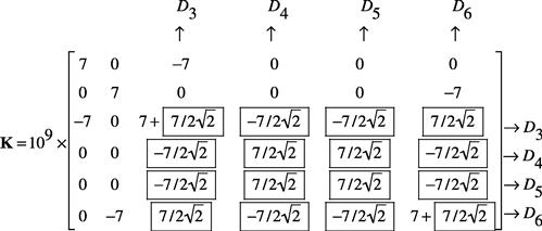 (4.52)
 (4.53)
The direct assembly process shown above is very simple, and can be coded in a computer program very easily. All one needs to do is add entries of the element matrix to the corresponding entries in the global stiffness matrix. The correspondence is usually facilitated using a so-called index that gives the relation between the element number and the global nodal numbers.
One may now ask how one can simply add up element matrices into the global matrix like this, and whether we can prove that this will indeed lead to the global stiffness matrix. The answer is that we can, and the proof can be performed simply using the equilibrium conditions at all of these nodes in the entire problem domain. The following gives such a simple proof.
We choose to prove the assembled result of the entries of the third row in the global stiffness matrix given in Eq. (4.53). The proof process applies exactly to all other rows. For the third row of the equation, we consider the equilibrium of forces in the x-direction at node 2 of elements 1 and 3, which corresponds to the third global DOF of the truss structure that links elements 1 and 3. For static problems, the FE equation for element 1 can be written in the following general form (in the global coordinate system):
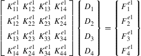 (4.54)
The third equation of Eq. (4.54), which corresponds to the third global DOF, is
![]() (4.55)
(4.55)
The FE equation for element 3 can be written in the following general form:
 (4.56)
The first equation of Eq. (4.54), which corresponds to the third global DOF, is
![]() (4.57)
(4.57)
Forces in the x-direction applied at node 2 consist of element force ![]() from element 1 and
from element 1 and ![]() from element 3, and the possible external force F3. All these forces have to satisfy the following equilibrium equation:
from element 3, and the possible external force F3. All these forces have to satisfy the following equilibrium equation:
![]() (4.58)
(4.58)
Substitution of Eqs. (4.55) and (4.57) into the above equation leads to
![]() (4.59)
(4.59)
This confirms that the coefficients on the left-hand side of the above equations are the entries for the third row of the global stiffness matrix given in Eq. (4.53). The above proof process is also valid for all the other rows of entries in the global stiffness matrix.
Step 4: Applying boundary conditions
The global matrix can normally be reduced in size after applying boundary conditions. In this case, D1, D2, and D5 are constrained, and thus
![]() (4.60)
(4.60)
This implies that the first, second, and fifth rows and columns will actually have no effect on the solving of the matrix equation. Hence, we can simply remove the corresponding rows and columns:
 (4.61)
The condensed global matrix becomes a 3 × 3 matrix, given as follows:
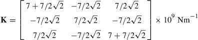 (4.62)
It can easily be confirmed that this condensed stiffness matrix is SPD. The constrained global FE equation is
![]() (4.63)
(4.63)
where
![]() (4.64)
(4.64)
and the force vector F is given as
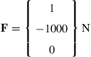 (4.65)
Note that the only force applied is at node 2 in the downward direction of D4. Equation (4.63) is actually equivalent to three simultaneous equations involving the three unknowns D3, D4, and D6, as shown below:
 (4.66)
Step 5: Solving the FE matrix equation
The final step would be to solve the FE equation, Eqs. (4.63), (4.66), to obtain the solution for D3, D4, and D6. Solving this equation manually is possible, since this only involves three unknowns in three equations. To this end, we obtain
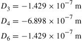 (4.67)
To obtain the stresses in the elements, Eq. (4.37) is used as follows:
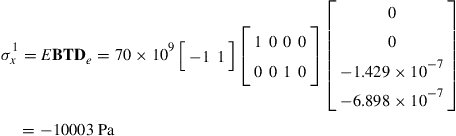 (4.68)
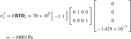 (4.69)
 (4.70)
In engineering practice, the problem can be of a much larger scale, and thus the unknowns or number of DOFs will also be very much more. Therefore, efficient equation solvers for FEM equations have to be used. Typical real-life engineering problems might involve hundreds of thousands, and even millions, of DOFs. Many kinds of such solvers are routinely available in math or numerical libraries in computer systems.
4.4 High order one-dimensional elements
For truss members that are free of body forces, there is no need to use higher order elements, as the linear element can already give the exact solution, as shown in Example 4.1. However, for truss members subjected to body forces arbitrarily distributed in the truss elements along their axial direction, higher order elements can be used for more accurate analysis. The procedure for developing such high order one-dimensional elements is the same as for the linear elements. The only difference is the shape function.
In deriving high order shape functions, we usually use the natural coordinate ξ, instead of the physical coordinate x. The natural coordinate ξ is defined as
![]() (4.71)
(4.71)
where xc is the physical coordinate of the mid-point of the one-dimensional element. In the natural coordinate system, the element is defined in the range of −1 ≤ξ ≤ 1. Figure 4.7 shows a one-dimensional element of nth order with (n + 1) nodes. The shape function of the element can be written in the following form using so-called Lagrange interpolants:
![]() (4.72)
(4.72)
where ![]() is the well-known Lagrange interpolant, defined as
is the well-known Lagrange interpolant, defined as
![]() (4.73)
(4.73)
Note in this definition that the subscript starts from zero. From Eq. (4.73), it is clear that
 (4.74)
Therefore, the high order shape functions defined by Eq. (4.72) are of the delta function property.

Using Eq. (4.73), the quadratic one-dimensional element with three nodes shown in Figure 4.8a can be obtained explicitly as
 (4.75)
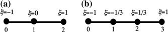
Figure 4.8 One-dimensional quadratic and cubic element with evenly distributed nodes. (a) Quadratic element; (b) cubic element.
The cubic one-dimensional element with four nodes shown in Figure 4.8b can be obtained as
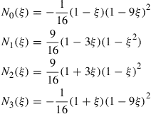 (4.76)
4.5 Review questions
1. What are the characteristics of the joints in a truss structure and what are the effects of this on the deformation and stress properties in a truss element?
2. How many DOFs does a 2-nodal planar truss element have in its local coordinate system, and in the global coordinate system? Why is there a difference in DOFs in these two coordinate systems?
3. How many DOFs does a 2-nodal space truss element have in its local coordinate system, and in the global coordinate system? Why is there such a difference?
4. Derive the expression for all the entries for the expression for the element stiffness matrix, ke, with Young’s modulus, E, length, le, and cross-sectional area, A = 0.02x + 0.01. (Note: non-uniform cross-sectional area.)
5. Derive the expression for all the entries for the expression for the element mass matrix, me, with the same properties as that in question 4 above.
6. Figure 4.9 shows a one-dimensional bar of length L and constant cross-sectional area A. The bar is made of functionally graded material (FGM). The Young’s modulus of the FGM material E(x) varies in the axial direction (x-direction). The bar is subjected to a uniformly distributed axial force F. The governing equation for the static problem of the bar is given by
![]()
where u is the unknown axial displacement, and Young’s modulus of the bar is given by
![]()
where E0 and Eg are given constants.
a. Develop the finite element equations for a two-node linear element of length L.
b. Discuss the results obtained.

7. Figure 4.10 shows a simple truss structure made of 3 members along the horizontal direction. The cross-sectional area, Young’s modulus, and length are denoted as A, E, and L, respectively. Using FEM and 3 linear 1D elements:
a. Give the global stiffness matrix K, in terms of A1, A2, A3, E1, E2, E3, L1, L2, and L3, without considering boundary condition.
b. Consider now nodes 1 and 4 are fixed, and let A1 = A2 = A3 = A, E1 = E2 = E3 = E, and L1 = L2 = L3 = L. A force P acts at node 3 in the horizontal direction. Find expressions for the displacements at nodes 2 and 3 in terms of A, E, L, and P.

8. Work out the displacements and the stresses of the truss structure shown in Figure 4.11. All the truss members are of the same material (E = 69.0 GPa) and with the same cross-sectional area of 0.01 m2.

9. Figure 4.12 shows a truss structure with 5 uniform members made of the same material. The cross-sectional area of all the truss members is 0.01 m2, and the Young’s modulus of the material is 2.1E11 N/m2. Using the finite element method:
a. Calculate all the nodal displacements.
b. Calculate the internal forces of all the truss members.
c. Calculate the reaction forces at all the supports.
10. Figure 4.13 indeed showed a simply supported structure with five uniform members made of the same material. The cross-sectional area of all the truss members is 0.01 m2, and the Young’s modulus of the material is 2.1E11 N/m2. Using the finite element method:
a. Calculate all the nodal displacements.
b. Calculate the internal forces of all the truss members.
c. Calculate the reaction forces at the supports.

11. Figure 4.14 shows a truss structure consisting of 4 truss members of the same dimensions. It is made of the same material with the Young’s modulus E = 210.0 GPa. The cross-sectional area of the truss members is 0.001 m2. Using the finite element method calculate:
a. The nodal displacement at node 2.
b. The reaction forces at all the supports.
c. The internal forces in all the truss members.
12. Figure 4.15 shows a three-node truss element of length L and a constant cross-sectional area A. It is made of a material of Young’s modulus E and density ρ. The truss is subjected to a uniformly distributed force b:
a. Derive the stiffness matrix for the element.
b. Write down the expression for the element mass matrix, and obtain m11 in terms of L, E, ρ, and A.
c. Derive the external force vector.

13. Figure 4.16 shows a truss structure with two uniform members made of the same material. The truss structure is constrained at two ends. The cross-sectional area of all the truss members is 0.01 m2, and the Young’s modulus of the material is 2.0E10 N/m2. Using the finite element method, calculate:
a. All the nodal displacements.
b. The internal forces in all the truss members.
c. The reaction forces at the supports.

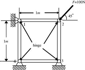
14. Figure 4.17 shows two identical vertical truss members connected by a ridged horizontal bar. These three members are hinged together at nodes 1, 3, and 4. All the members are of length L = 2a, cross-sectional area A, and Young’s modulus E. Two forces are applied vertically at nodes 1 and 4. Using ONE truss element:
a. Calculate the displacements at nodes 1 and 4, if any, in terms of F, L (or a), A, and E.
b. Calculate the reaction forces at nodes 3, 2, and 5, if any, in terms of F, L (or a), A, and E.

References
1. Liu GR, Nguyen Thoi Trung. Smoothed Finite Element Methods. Boca Raton: CRC Press; 2010.
2. Rao SS. The Finite Element in Engineering. third ed. Butterworth-Heinemann 1999.
3. Reddy JN. Finite Element Method. New York: John Wiley & Sons Inc.; 1993.
4. Zienkiewicz OC, Taylor RL. The Finite Element Method. fifth ed. Butterworth-Heinemann 2000.