
Computational Modeling
1.1 Introduction
The Finite Element Method (FEM) has developed into a key indispensable technology in the modeling and simulation of advanced engineering systems in various fields like housing, transportation, communications, and so on. In building an advanced engineering system, engineers and designers go through a sophisticated process of modeling, simulation, visualization, analysis, design, prototyping, testing, and lastly, fabrication. More often than not, much work is involved before the fabrication of the final product or system. This is to ensure the workability of the finished product, as well as for cost effectiveness in the manufacturing process. This process is illustrated as a flowchart in Figure 1.1. It is often iterative in nature, meaning that some of the procedures are repeated based on the results obtained at a current stage, so as to achieve an optimal performance at the lowest cost for the system to be built. Therefore, techniques related to modeling and simulation in a rapid and effective way play an increasingly important role, and the FEM becomes very much a standard tool in any major development of a system or product.

This book deals with topics related mainly to modeling and simulation, which are underscored in Figure 1.1. The focus will be on the techniques of physical, mathematical, and computational modeling, and other aspects of computational simulation. A good understanding of these techniques plays an important role in building an advanced engineering system in a rapid and cost-effective way.
So what is the FEM? The FEM was first used to solve problems of solid and structural analysis, and has since been applied to many problems like thermal analysis, fluid flow analysis, piezoelectric analysis, and many others. Basically, the analyst seeks to determine the distribution of some field variable, for example, the displacement in structural mechanics analysis, the temperature or heat flux in thermal analysis, the electrical charge in electrical analysis, and so on. The FEM is a numerical method that seeks an approximated solution of the distribution of field variables in the problem domain that is often difficult to obtain analytically. It is done by first dividing the problem domain into a number of small pieces called elements, often of simple geometry, as shown in Figures 1.2 and 1.3. Physical principles/laws are then applied to each small element. Figure 1.4 shows a schematic illustration of a distribution of a field, F(x), in one dimension that is approximated using the FEM. In this case, F(x) is a continuous function that is approximated using piecewise linear functions in an element. In this one-dimensional case, the ends of each element are termed nodes. The unknown variables in the FEM are simply the discrete values of the field variable at the nodes. Physical and mathematical principles are then followed to establish governing equations for each element, after which the elements are “tied” to one another to describe the distribution of the field in the entire geometry. This process leads to a set of linear algebraic simultaneous equations for the entire system that can be solved easily to yield the required field variable.
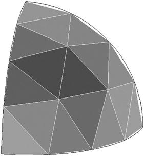

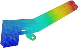
Figure 1.3 Mesh for the design of a scaled model of an aircraft for dynamic testing in the laboratory (Quek 1997–98).
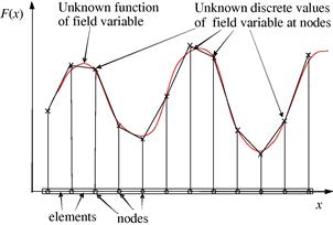
Figure 1.4 Finite element approximation for a one-dimensional case. A continuous function is approximated using piecewise linear functions in each sub-domain/element.
This book aims to bring across the various concepts, methods, and principles used in the formulation of FE equations in a manner that is easy to understand. Worked examples and case studies using the well-known commercial software package ABAQUS and ANSYS will be discussed, and effective techniques and procedures will be highlighted.
1.2 Physical problems in engineering
There are numerous physical problems in an engineering system. As mentioned earlier, although the FEM was initially used for solid and structural analysis, many other physical problems can be solved using the FEM. Mathematical models of the FEM have been formulated for the numerous physical phenomena that occur in engineering systems. Common physical problems solved using the standard FEM include:
This book first focuses on the formulation of finite element equations for the mechanics of solids and structures, since that is what the FEM was initially designed for. FEM formulations for heat transfer problems are then described. Nevertheless, the conceptual understanding of the methodology of the FEM is the most important and will be emphasized in both solid mechanics and heat transfer problems. The application of the FEM to all other physical problems utilizes similar concepts.
Computer modeling using the FEM consists of the major steps discussed in the next section.
1.3 Computational modeling using FEM
The behavior of a physical phenomenon in a system depends upon the geometry or domain of the system, the property of the material or medium, and the boundary, initial, and loading conditions. For an engineering system, the geometry or domain can be very complex. Furthermore, the boundary and initial conditions can also be very complicated. It is therefore, in general, very difficult to solve the governing differential equation via analytical means. In practice, most of the problems are solved using numerical methods. Among these, the methods of domain discretization championed by the FEM are the most popular due to their reliability, practicality, versatility, and robustness.
The procedure of computational modeling using the FEM broadly consists of four steps:
1.3.1 Modeling of the geometry
Most physical structures, components or domains are in general very complicated, and usually made up of multiple components. One can imagine the complexity that goes into making an automobile, an aircraft, an ocean-going vessel, and so on. It is therefore common, and often a good practice, to simplify parts of the geometry so that modeling is more manageable. The geometry and boundary of a structure can be made up of curved surfaces/lines, but as we perform FEM based modeling, it is important to bear in mind that the geometry is eventually represented by a collection of elements, and the curved lines/surfaces may be approximated by piecewise straight lines or flat surfaces, if these elements are assumed to be flat/straight pieces/segments (that is, linearity is assumed). Figure 1.2 shows an example of a curved boundary represented by the straight lines of the edges of triangular elements. The accuracy of the representation of the curved part, as in Figure 1.2, is controlled by the number of elements used. It is obvious that with more elements, the representation of the curved parts by straight edges would be smoother and more accurate. On the other hand, with more elements, longer computational time is required. Unfortunately, modelers often face constraints in terms of available computational resources and it is often necessary to limit the number of elements used in the model. As such, compromises are usually made in order to decide on an optimum number of elements used. These compromises usually result in the omission of fine details of the geometry unless very accurate results are required for those regions. The analysts will then have to interpret the results of the simulation with these geometric approximations in mind.
Depending on the software used, there are many ways to create a proper geometry in the computer for the FE mesh. Points can be created simply by keying in the coordinates. Lines and curves can be created by connecting the points or nodes. Surfaces can be created by connecting, rotating or translating the existing lines or curves. Solids can be created by various operations of connecting, rotating or translating the existing surfaces. Points, lines and curves, surfaces and solids can be translated, rotated or reflected to form new ones.
More often than not, the use of a graphic interface helps in the creation and manipulation of the geometrical objects on computers. There are numerous Computer Aided Design (CAD) software packages used for engineering design. These CAD packages can generate appropriate files containing the geometry of the designed engineering system and these files can then be read by modeling software packages, in which appropriate discretization of the geometry into elements can be carried out. However, in many cases, complex objects read directly from a CAD file may need to be modified and simplified before performing discretization. It may be worth mentioning that there are CAD packages which incorporate modeling and simulation packages, and these are useful for the rapid prototyping of new products.
While most modeling software packages try to make modeling a breeze by developing excellent user interfaces, it is equally important to have knowledge, experience, and good engineering judgment. This is what distinguishes a good modeler from one who is just proficient in using the software. For example, finely detailed geometrical features often only play an aesthetic role, and have negligible effects on the functional performance of the engineering system. These features can sometimes be omitted, ignored or simplified, but it takes good engineering judgment to decide if any geometrical assumptions/simplifications will have a negligible effect on the overall simulation results.
Possessing sufficient knowledge and engineering judgment enables one to recognize a physical component, and possibly simplify that component mathematically, so that modeling can be more effective. For example, a plate has three dimensions geometrically. The plate in the plate theory of mechanics is represented mathematically only in two dimensions (the reason for this will be elaborated in Chapter 2). Therefore the geometry of a “mechanics” plate is a two-dimensional flat surface. Plate elements will be used in meshing these surfaces. A similar situation can be found in shells. A physical beam also has three dimensions. The beam in the beam theory of mechanics is represented mathematically in only one dimension, therefore the geometry of a “mechanics” beam is a one-dimensional straight line. Beam elements have to be used to mesh the lines in models. This is also true for truss structures. In fact, the entire physical world that we visualize in space is in three dimensions, yet there are often components like the plates, shells, beams, and so on that we can approximate with a lower dimension that makes modeling so much easier and still provides acceptable accuracy for engineering design purposes.
1.3.2 Meshing
When we discretize the geometry or domain into small pieces which we have come to call elements or cells, the process is called meshing. Why do we mesh? The rationale behind this is in fact based on a very logical understanding. We can expect the solution for an engineering problem to be very complex, and to vary in a way that is very unpredictable using functions across the whole domain of the problem. However, if the problem domain can be divided (meshed) into small elements or cells using a set of grids or nodes, the variation of the solution within an element can be approximated very easily using simple functions such as polynomials. The collective variations of the solutions for all of the elements thus form the variation of the solution for the whole problem domain.
Proper theories are needed for discretizing the governing equations based on the discretized domains. The theories used are different from problem to problem, and will be covered in detail in this book for various types of problems. But before that, we need to generate a mesh for the problem domain.
Mesh generation is a very important task in pre-processing. It can be a very time consuming task to the analyst, and usually an experienced analyst will produce a more credible mesh for a complex problem. The domain has to be meshed properly into elements of specific shapes such as triangles and quadrilaterals in 2D, and tetrahedrons and hexahedrons in 3D. Information such as element connectivity must be created during the meshing for use later in the formation of the FEM equations. It is ideal to have a fully automated mesh generator, which by itself is a big research field, but at this moment, it is still not commercially available. A semi-automatic mesh generator is available in most pre-processors as part of commercial FEM software packages. There are also packages designed mainly for meshing. Such packages can generate files of a mesh, which can be read by other modeling and simulation packages.
Triangulation is the most flexible and well-established way to create meshes with triangular elements. It can be made almost fully automated for two-dimensional planes and even three-dimensional spaces. Therefore it is commonly available in most pre-processors. The additional advantage of using triangles is the flexibility in adapting complex geometry and its boundaries. One can easily visualize fitting triangles into an acute corner of geometry, but it will be less obvious how one can do it with, say, quadrilateral elements without severely distorting the elements. However, the disadvantage of using triangle elements is that the accuracy of the simulation results based on triangular elements is often significantly lower1 than that obtained using quadrilateral elements. Quadrilateral element meshes are in general more difficult to generate in an automated manner. Some examples of meshed solids and structures are given in Figures 1.3–1.7.


1.3.3 Material or medium properties
Many engineering systems consist of multiple components and each component can be of a different material. In fact, even within a single component, there can be multiple materials, as in the case of a composite material. Properties of materials can therefore be defined for a group of elements or even for individual elements if needed. The FEM can therefore work very conveniently for systems with multiple materials, which is a significant advantage of the FEM. For different phenomena or physics to be simulated, different sets of material properties are required. For example, Young’s modulus and shear modulus are required for the stress analysis of solids and structures, whereas the thermal conductivity coefficient will be required for a thermal analysis. The input of material properties into a pre-processor is usually straightforward; all the analyst needs to do is to key in the relevant inputs (usually with a convenient user interface) for the required material properties and specify to which region of the geometry or which elements the data applies. Nevertheless, obtaining these properties is not always easy. There are commercially available material databases for standardized materials, but experiments are usually required to accurately determine the property of special materials to be used in the system. In some cases, perhaps another simulation (at a smaller length scale, like molecular dynamics simulation and/or quantum mechanics-based first principles calculations) is required to first obtain the material’s properties, which are then used as inputs for the FEM model. This, however, is beyond the scope of this book, and throughout, we simply assume that the material property is known.
1.3.4 Boundary, initial, and loading conditions
Boundary, initial, and loading conditions play a decisive role in the simulation. Prescribing these conditions is usually done easily using commercial pre-processors, and it is often interfaced with graphics. Users can specify these conditions either to the geometrical identities (points, lines or curves, surfaces, and solids) or to the mesh identities (nodes, elements, element edges, element surfaces). Again, to accurately simulate these conditions for actual engineering systems requires experience, knowledge, and proper engineering judgments. The boundary, initial, and loading conditions are different from problem to problem, and will be covered in detail in subsequent chapters.
1.4 Solution procedure
1.4.1 Discrete system equations
Based on the mesh generated, a set of discrete simultaneous system equations can be formulated using existing approaches. There are a few types of approach for establishing the simultaneous equations. The first is based on energy principles, such as Hamilton’s principle (Chapter 3), the minimum potential energy principle, and so on. The traditional FEM is established based on these principles. The second approach is the weighted residual method, which is also often used for establishing FEM equations for many physical problems, and will be demonstrated for heat transfer problems in Chapter 12. The third approach is based on the Taylor series, which led to the formation of the traditional Finite Difference Method (FDM). The fourth approach is based on the control of conservation laws on each finite volume (elements) in the domain. The Finite Volume Method (FVM) is established using this approach. Another approach is by integral representation used in some mesh-free methods (Liu, 2009), in particular the Smoothed Particle Hydrodynamics (SPH) method (Liu and Liu, 2003). Engineering practice has so far shown that the first two approaches are most often used for solid and structures, and the other two approaches are often used for fluid flow simulation. However, the FEM has also been used to develop commercial packages for fluid flow and heat transfer problems, and FDM can be used for solids and structures. It is interesting to note, without going into detail, that the mathematical foundation of all these approaches can be based on the residual method. An appropriate choice of the “test” and “trial” functions in the residual method can lead to the FEM, FDM or FVM formulation.
This book first focuses on the formulation of finite element equations for the mechanics of solids and structures based on energy principles. FEM formulations for heat transfer problems are then described so as to demonstrate how the weighted residual method can be used for deriving FEM equations. This will provide the basic knowledge and key approaches into the FEM for dealing with other physical problems.
1.4.2 Equation solvers
After an FEM model has been created, it is then fed into a solver to solve the discretized system of equations—simultaneous equations for the field variables at the nodes of the mesh. This is the most computer hardware-demanding process. Different software packages use different algorithms depending upon the physical phenomenon to be simulated. There are two very important considerations when choosing algorithms for solving a system of equations: One is the storage required, and another is the central processing unit (CPU) time needed.
There are two main types of method for solving simultaneous equations: direct methods and iterative methods. Commonly used direct methods include the Gauss elimination method and the LU decomposition method (factorizing a matrix into a product of a Lower triangular matrix and a Upper triangular matrix). Those methods work well for relatively small equation systems. Direct methods operate on fully assembled system equations, and therefore demand far larger storage space. It can also be coded in such a way that the assembling of the equations is done only for those elements involved in the current stage of equation solving. This can reduce the requirements on storage significantly.
Iterative methods include the Gauss-Jacobi method, the Gauss-Seidel method, the successive over-relaxation (SOR) method, generalized conjugate residual methods, the line relaxation method, and so on. These methods work well for relatively larger systems. Iterative methods are often coded in such a way as to avoid full assembly of the system matrices in order to save significantly on the storage. The performance in terms of the rate of convergence of these methods is usually problem dependent. In using iterative methods, pre-conditioning plays a very important role in accelerating the convergence process. For nonlinear problems, another iterative loop is needed. The nonlinear equation has to be properly formulated (linearized) into a set of linear equations through the iterations of the extra iterative loop.
For time-dependent problems, time stepping is necessary. Starting from the given initial state, the time history of the solution is computed by marching forward to the next time steps until the desired time is reached. There are two main approaches to time stepping: the implicit and explicit approaches. Implicit approaches are usually more stable numerically but less efficient computationally than explicit approaches for one step. Moreover, contact algorithms can be developed easily using explicit methods. Details of these issues will be given in Chapter 3.
1.5 Results visualization
The result generated after solving the system equation usually comprises a vast volume of digital data. The results have to be visualized in such a way that it is easy to interpolate, analyze, and present. The visualization is performed through a so-called post-processor usually packaged together with the software. Most of these processors allow the user to display 3D objects in many convenient and colorful ways on screen. The object can be displayed in the form of wire-frames, groups of elements, and groups of nodes. The user can rotate, translate, and zoom into and out from the objects. Field variables can be plotted on the object in the form of contours, fringes, wire-frames, and deformations. Usually, there are also tools available for the user to produce iso-surfaces, or vector fields of variables. Tools to enhance visual effects are also available, such as shading, lighting, and shrinking. Animations and movies can also be produced to simulate the dynamic aspects of a problem. Outputs in the form of tables, text files, and x-y plots are also routinely available. Throughout this book, worked examples with various post-processed results are given.
Advanced visualization tools, such as virtual reality and 3D visualization, are available nowadays. These advanced tools allow users to display objects and results in a much more realistic 3D form. The platform can be a goggle, inversion desk or even a room. When the object is immersed in a room, analysts can walk through the object, go to the exact location and view the results. Figures 1.8 and 1.9 show an airflow field in a virtually designed building.

Figure 1.8 Immersed, 3D visualization of air flow field in virtually designed building. (Courtesy of the Institute of High Performance Computing.)
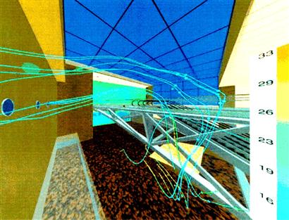
Figure 1.9 A 3D rendition of air flow in a virtually designed building system. (Courtesy of the Institute of High Performance Computing.)
To summarize, this chapter has briefly given an overview of the steps involved in computer modeling and simulation using FEM. With rapidly advancing computer technology, using FEM with the aid of computers is indispensable in any design process of an advanced engineering system. Software developers have been making it easier and more user-friendly for anyone to use simulation software. The subsequent chapters in this book will discuss the “behind-the-scenes” processes that the software is developed to execute when an engineer sits in front of the computer and performs an FEM analysis.
Reference
1. Liu GR. Meshfree Methods: Moving Beyond the Finite Element Method. second ed. Boca Raton: CRC Press; 2009.
2. Liu GR, Liu MB. Smoothed Particle Hydrodynamics: A Meshfree Particle Method. World Scientific Publishing Company 2003.
1This has been overcome by the Smoothed Finite Element methods (S-FEM). See Liu and Trung, Smoothed Finite Element Methods, CRC Press, 2010.