
Using FEM Software Packages
13.1 Introduction
Realistic finite element problems might consist of hundreds of thousands and even several millions of elements and nodes and, therefore, they are usually solved in practice using commercially available software packages. There are currently a large number of commercial software packages available for solving a wide range of problems: Solid and structural mechanics, heat and mass transfer, fluid mechanics, acoustics and multi-physics, which might be static, dynamic, linear or non-linear. Most of these software packages use the FEM as a stand-alone approach or combine it with other numerical methods to solve physical problems. All FEM software packages are developed based on the same basic methodology described in this book, but usually extend their capabilities for more complex problems with the development of detailed and fine-tuned algorithms and numerical schemes. Table 13.1 lists some of the commercially available software packages using FEM, the finite volume method (FVM), and the boundary element method (BEM). This chapter introduces the use of an FEM package primarily through ABAQUS FEA®, currently owned by Dassault Systèmes, due to its strong capabilities, in general, in dealing with non-linear problems. At the end of the chapter, we also remark on the modeling similarities across FEM packages by highlighting basic steps using a graphical user interface (GUI) via another popular FEM package, ANSYS.
Table 13.1
Some of the commercially available software packages.
| Software Package | Methods Used | Application Problems |
| ABAQUS | FEM (implicit, explicit) | Structural analysis, acoustics, thermal analysis |
| ANSYS | FEM (implicit, explicit) | Structural analysis, acoustics, thermal analysis, multi-physics |
| I-deas | FEM (implicit) | Structural analysis, acoustics, thermal analysis |
| LS-DYNA | FEM (explicit) | Structural dynamics, computational fluid dynamics, fluid-structural interaction |
| Sysnoise | FEM/BEM | Acoustics (frequency domain) |
| NASTRAN | FEM (implicit) | Structural analysis, acoustics, thermal analysis |
| MARC | FEM (implicit) | Structural analysis, acoustics, thermal analysis |
| MSC-DYTRAN | FEM + FVM (explicit) | Structural dynamics, computational fluid dynamics, fluid-structural interaction |
| ADINA | FEM (implicit) | Structural analysis, computational fluid dynamics, Fluid-structural interaction |
With the development of convenient user interfaces, most finite element software can be used as a “black box” by users without extensive knowledge of FEM. The authors have witnessed many cases where the FEM packages were misused, resulting in what is termed “garbage in, garbage out” simulations. The danger here is that the “garbage” output is often obscured by beautiful pictures and animations that can lead to erroneous decisions in designing an engineering system.
An understanding of the materials covered in the previous chapters in this book should shed some light into this black box, leading to the proper use of most software packages. As mentioned, this chapter will primarily use ABAQUS FEA as an example to highlight the general steps involved in using commercial software packages from a user point of view. Chapters 1 to 12 have highlighted various basic concepts in the finite element method and the case studies actually relate these concepts to examples solved using typical FEM packages (primarily ABAQUS/Standard). There are other modules in the ABAQUS finite element package including ABAQUS/Explicit, ABAQUS/CFD, and ABAQUS/CAE. ABAQUS/Explicit is used for mainly explicit dynamic analysis. ABAQUS/CFD provides computational fluid dynamics capabilities. ABAQUS/CAE is an interactive pre- and post-processor that can be used to create finite element models and the associated input file for ABAQUS. In this chapter, however, the focus will be on the writing of a basic ABAQUS/Standard input file and ABAQUS/Standard will from now on just be called ABAQUS. This book cannot and will not try to in any way replace the extensive and excellent manuals provided together with the ABAQUS software. This chapter will just serve as a general guide especially suited for beginner users to have a quick understanding of using an FEM package, without going through the often daunting details covered in comprehensive user manuals. It is hoped that, after reading this chapter, readers will have an even better understanding of the basic finite element concepts being implemented in finite element software packages.
13.2 Basic building block: keywords and data lines
The first step to writing an ABAQUS input file is to know the way data is included in the input file. In ABAQUS, the data definitions are expressed in what are termed option blocks or groups of cards. Basically, it is thus named because the user has the option to choose particular data blocks that are relevant for the model to be defined. Each option block can be considered to be a basic building block that builds up the entire input file. The option block is introduced by a keyword line and if the option block requires data lines, these will follow directly below the keyword line. The general layout of a particular option block is shown below with the definition of beam elements as an example:

Keyword lines begin with an asterisk, *, followed by the name of the block. In this case, we define elements in the element block identified with the keyword, ELEMENT. Subsequent information on the keyword line provides additional parameters associated with the block being used. In this case, it is necessary to tell ABAQUS what type of element is being used (B23 – 2 node, 1D Euler-Bernoulli beam element) and the elements are grouped into a particular set with the arbitrary given name, “BEAM.” This grouping of entities into sets is a very convenient tool, which the analyst will use very often. It enables the analyst to make references to the set when defining certain option blocks.
The data lines basically provide data, if required, that is associated with the option block used. In the above example, element identification (i.d.), and the nodes that make up the element are the necessary data required. Note that the information provided in the data lines would vary with some of the parameters defined in the keyword line. For example, if the element type being used is a 2D plane stress element, then the data lines would require different data as shown below.

Note that in this case, the element type CPS4 which represents 4-nodal, 2D solid elements is being used and, correspondingly, the data lines must include the element i.d. (as before), and four nodes that make up each element instead of two for the case of the beam element previously.
13.3 Using sets
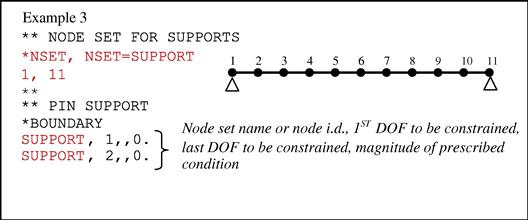
In the last section, it can be seen in Eg. 1 that elements can be grouped into a set for future reference by other option blocks. A set can be a grouping of nodes or a grouping of elements. The analyst will usually provide a name for the set that contains between 1 to 80 characters. For example, in Eg. 1 above, “BEAM” is the name of the set containing elements 1 and 2; and in Eg. 2, “PLSTRESS” is the name of the set containing elements 1 and 2. In both examples, the sets are defined together with the definition of the elements themselves in the element block. However, sets can also be defined as a separate block on their own. In Eg. 3 below, the pinned support of the 1D beam is to be defined. Nodes 1 and 11 (provided in the data line for the “NSET” block) are first grouped in the node set called “SUPPORT.” Then using the “BOUNDARY” option block, the node set, “SUPPORT” is referenced to constrain the DOFs 1 and 2 (x translation and y translation) to zero. In other words, rather than having four data lines for the two nodes 1 and 11 (each node having to constrain two DOFs), we now have only two lines with the reference to the node set support. Another thing to note in this example is the usage of comment lines. Comment lines exist in ABAQUS too just like in most programming languages. Comment lines begin with two asterisks, **, and whatever follows in that line after the asterisks will not be read by ABAQUS as input information defining the model.
This is of course a very simple case and the reduction of the number of data lines from four to two may not seem very significant. However, imagine if it were a huge 3D model and one whole surface containing about 100 nodes were to be prescribed a boundary condition. If the nodes on this surface were not grouped up into node sets, then the user would end up with 100 × (No. of DOFs to be constrained) data lines just to prescribe a boundary condition. A more efficient way of course is to group the nodes in this particular surface in a node set and then, as in the above example, write down the data lines referencing the node set to be constrained. In this way, the number of data lines for the “BOUNDARY” block would be equal to the number of DOFs to be constrained. Similar usage of sets can be applied to elements as well. One common usage of element sets (ELSET) is the referencing of element properties to the elements in a particular set (see example in Section 13.5.3). Sets are thus the basic referencing tool in ABAQUS.
13.4 ABAQUS input syntax rules
The previous section has introduced the way data are organized in the ABAQUS input file. Like most programming language, there are certain rules which the entries into the input file must follow. A violation of these rules would generally result in a syntax error when ABAQUS is run, and most of the time, the analysis will not be carried out. So far, it has been briefed that ABAQUS generally has three types of entries in the input file: the keyword lines, the data lines, and the comment lines. Comment lines generally do not need many rules except that they must begin with two asterisks (**) in columns 1 and 2. This section therefore describes the rules that apply to all keyword and data lines.
13.4.1 Keyword lines
The following rules apply when entering a keyword line:
• The first non-blank character of each keyword line must be an asterisk (*).
• The keyword must be followed by a comma (,), if any further parameters are to be included in the line.
• Parameters are separated by commas.
• Blanks on a keyword line are ignored.
• A line can include no more than 256 characters including blanks.
• Keywords and parameters are not case sensitive.
• Parameter values are usually not case sensitive. The only exceptions to this rule are those imposed externally to ABAQUS, such as file names on case-sensitive operating systems.
• If a parameter has a value, the equal sign (=) is used. The value can be an integer, a floating point number, or a character string, depending on the context. For example,
![]()
• Continuation of a keyword line is sometimes necessary especially when there are a large number of parameters. If the last character of a keyword line is a comma, the next line is treated as a continuation line. For example, the example stated in the previous rule can also be written as
![]()
13.4.2 Data lines
The data lines must immediately follow a keyword line if they are required. The following rules apply when entering a data line:
1. A data line can include no more than 256 characters including blanks.
2. All data items are separated by commas. An empty data field is specified by omitting data between commas. ABAQUS will use values of zeros for any required numeric data that are omitted unless there is a default value allocated. If a data line contains only a single data item, the data item should be followed by a comma.
3. A line must contain only the number of items specified.
4. Empty data fields at the end of a line can be ignored.
5. Floating point numbers can occupy a maximum of 20 spaces including the sign, decimal point, and any exponential notation.
6. Floating point numbers can be given with or without an exponent. Any exponent, if input, must be preceded by E or D and an optional (–) or (+) to indicate the sign of the exponent.
7. Integer data items can occupy a maximum of 10 digits.
8. Character strings can be up to 80 characters long and are not case sensitive.
9. Continuation lines are allowed in specific instances such as when defining elements with a large numbers of nodes. If allowed, such lines are indicated by a comma as the last character of the preceding line.
13.4.3 Labels
Examples of labels are set names, surface names and material names and they are case sensitive unlike the other entries in the keyword line. Labels can be up to 80 characters long. All spaces within a label are ignored unless the label is enclosed in quotation marks, in which case all spaces within the label are maintained. A label that is not enclosed within quotation marks may not include a period (.) and should not contain characters such as commas and equal signs. If a label is defined using quotation marks, the quotation marks are stored as part of the label. Any subsequent reference or use of the label should also include the quotation marks. Labels cannot begin and end with a double underscore (e.g., __ALU__). This label format is reserved for use internally within ABAQUS.
13.5 Defining a finite element model in ABAQUS
Though very often, the use of a GUI such as in ABAQUS/CAE or PATRAN can be helpful in creating the finite element model and generating the input file for complex models, the analyst may still find certain limitations in pre-processors whereby certain functions, element types, material definitions, and other modeling requirements cannot be automatically defined. Many times, a specific analysis will require more than just the usual analysis steps and this is when an analyst will find that knowing the basic concepts of writing an input file will enable him or her to either write a whole input file for the specific problem or to modify the existing input file that is generated by the pre-processor.
An ABAQUS input file is an ASCII data file and can be created or edited by using any text editor. The input file contains two main sets of data: model data and history data. The model data consists of data defining the finite element model. This part of the input file defines the elements, the nodes, the element properties, the material properties, and any other data relating to the model itself. Looking at the input files provided for the case studies included in previous chapters, it should be noted that all the data provided before the “*STEP” line is considered as the model data. The history data, on the other hand, defines what happens to the finite element model. It tells ABAQUS the events the model has gone through, the loadings the model have, the type of response that should be sought for, and so on. In ABAQUS, the history data is made up of one or more steps. Each step defines the analysis procedures by providing the required parameters. It is possible and in fact quite common to have multiple steps to define a whole analysis procedure. For example, to obtain a steady-state dynamic response due to a harmonic excitation at a given frequency by modal analysis, one must first obtain the eigenvalues and eigenvectors. This can be defined in a step defined by *FREQUENCY, which calls for the eigenvector extraction analysis procedure. Following that, another step defined by *STEADY STATE DYNAMICS is necessary that calls for the modal analysis procedure to solve for the response under a harmonic excitation. As such, the history data can be said to be made up of a series of steps, which in a way tells the history of the analysis procedure. This section will describe in more detail how a basic model can be defined in ABAQUS. Input files defining most problems have the same basic structure:
1. An input file must begin with the *HEADING option block, which is used to define a title for the analysis. Any number of data lines can be used to give the title.
2. After the heading lines, the input file would usually consist of the model data, which consists of the node definition, element definition, material definition, initial conditions, and so on.
3. Finally the input file would consist of the history data, in which is defined the analysis type, loading, output requests, and so on. Usually, the *STEP option is the dividing point in the input file between the model and history data. Everything appearing before the *STEP option will be considered model data and everything after will be considered the history data.
The following will list some of the options and data that can be included in the model and history data. This book will not elaborate on all the available options and, if required, the user is recommended to refer to the software’s user manual (ABAQUS keywords manual, 2000; ABAQUS user’s manual, 2000; ABAQUS theory manual, 2000). Elaboration will be done on some of the necessary options for a basic finite element model later.
13.5.1 Model data
Some of the items that must be included in the model data are as follows:
• Geometry of the model: The geometry of the model is described by its elements and nodes.
• Material definitions, which are usually associated with parts of the geometry.
Other optional data in the model data section are:
• Parts and an assembly: The geometry can be divided into parts, which are positioned relative to one another in an assembly.
• Initial conditions: Non-zero initial conditions such as initial stresses, temperatures, or velocities can be specified.
• Boundary conditions: Zero-valued boundary conditions (including symmetry conditions) can be imposed on the model.
• Constraints: Linear constraint equations or multipoint constraints can be defined.
• Contact interactions: Contact conditions between surfaces or parts can be defined.
• Amplitude definitions: Amplitude curves which the loads or boundary conditions are to follow can be defined.
• Output control: Options for controlling model definition output to the data file can be included.
• Environment properties: Environment properties such as the attributes of a fluid surrounding the model can be defined.
• User subroutines: User-defined subroutines, which allow the user to customize ABAQUS can be defined.
• Analysis continuation: It is possible to write restart data or to use the results from a previous analysis and continue the analysis with new a model or history data.
13.5.2 History data
As mentioned, in the history data, the entries are divided into steps. Each step will begin with the *STEP option and ends with the *END STEP option. There are generally two kinds of steps that can be defined in ABAQUS—the general response analysis steps (can be linear or non-linear); and the linear perturbation steps. A general analysis step is one in which the effects of any nonlinearities present in the model can be included. The starting condition for each general analysis step is the ending condition from the last general analysis step. The response of each general analysis step contributes to the overall history of the response of the model. A linear perturbation analysis step, on the other hand, is used to calculate the linear perturbation response from the base state. The base state is the present state of the model at the end of the last general analysis response. For the perturbation step, the response does not contribute to the history of the overall response and hence can be called for at any time in between general steps. For cases where the general step or the linear perturbation step is the first step, then the initial conditions defined will define the starting condition or the base state, respectively. Following is a list of the analysis types that use linear perturbation procedures:
• *BUCKLE (Eigenvalue buckling prediction)
• *FREQUENCY (Natural frequency extraction)
• *MODAL DYNAMIC (Transient modal dynamic analysis)
• *STEADY STATE DYNAMICS (Modal steady-state dynamic analysis)
• *STEADY STATE DYNAMICS, DIRECT (Direct steady-state analysis)
Except for the above analysis types and for the *STATIC (where both general and perturbation can be used), all other analysis types are general analysis steps.
Some of the data that must be included in the history data or within a step are:
• Analysis type: An option to define the analysis procedure type which ABAQUS will perform. This must appear immediately after the *STEP option.
Other optional data include:
• Loading: Some form of external loading can be defined. Loadings can be in the form of concentrated loads, distributed loads, thermal loads, and so on. Loadings can also be prescribed as a function of time following the amplitude curve defined in the model data. If an amplitude curve is not defined, ABAQUS will assume that the loading varies linearly over the step (ramp loading) or that the loading is applied instantaneously at the beginning of the step (step loading).
• Boundary conditions: Zero-valued or non-zero boundary conditions can be added, modified or removed. Note that if defined in the model data, only zero-valued and symmetrical boundary conditions can be included.
• Output control: Controls the requested output from the analysis. Output variables depend on the type of analysis and the type of elements used.
• Auxiliary controls: Options are provided to allow the user to overwrite the solution controls that are built into ABAQUS.
• Element and surface removal/reactivation: Portions of the model can be removed or reactivated from step to step.
13.5.3 An example of a cantilever beam problem
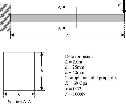
One of the best ways of learning about and understanding the ABAQUS input file is to follow an example. We will use a simple example of modeling a cantilever beam subjected to a downward force as shown in Figure 13.1. This problem can be modeled using 1D beam elements and the finite element model using an ABAQUS input file.
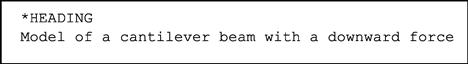
As mentioned, the first thing to include in the input file is the *HEADING option. The data line after the *HEADING keyword line briefly describes the problem.
Next we will write the model data. First, the nodes of the problem must be defined since elements must be made up of nodes and both nodes and elements make up the geometry of the problem.

Using the *NODE option, the nodes at the end are first defined. We then use the option *NGEN to generate evenly distributed nodes between the first and the last nodes. *NGEN is one of the several mesh generation capabilities provided by ABAQUS. We could also define all 11 nodes individually by specifying their coordinates, but using *NGEN would be more efficient for large problems. So we have now defined 11 nodes uniformly along the length of the beam. Next, the elements will be defined:

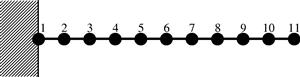
Here, the *ELEMENT option is used to define the first element that consists of nodes 1 and 2. The TYPE parameter is included to specify what type of element is being defined. In this case, B23 refers to a 1D beam element in a plane with cubic interpolation. Users can refer to the ABAQUS manual for the element library to check the codes for other element types. Similar to the definition of nodes, *ELGEN is used to generate 1 to 10 elements. The elements are then grouped into a node set called RECT_BEAM. This will make the referencing of element properties much easier later on. So, we have now defined 11 nodes and 10 elements (see Figure 13.2).
The next step will be to define the element properties:
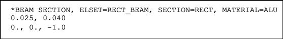
In the *BEAM SECTION keyword line, the element set RECT_BEAM defined earlier is now referenced, meaning that the elements grouped under RECT_BEAM will all have the properties defined in this option block. We also provide the information that the beam has a rectangular (RECT) cross-section. There are other cross-sections available in ABAQUS such as circular cross-sections (CIRC), trapezoidal cross-sections (TRAPEZOID), closed thin-walled sections (BOX, HEX, and PIPE), and open thin-walled sections (I-section, and L-section). ABAQUS also provides for a “general” cross-section by specifying geometrical quantities necessary to define the section. The material associated with the elements is also defined as aluminum (ALU), the properties of which will be defined later. It is a good time to note that, unlike most programming languages, the ABAQUS input file need not follow a top-down approach when ABAQUS is assessing the file. For example, the material ALU is already referenced at this point under the *BEAM SECTION option block though its material properties are actually defined further down the input file. There will not be any error stating that the material ALU is invalid regardless of where the material is defined, unless it is not defined at all throughout the input file. This is true for all other entries into the input file. Let us now look at the data lines. The first data line in the *BEAM SECTION basically defines the dimensions of the cross-section (0.025 m × 0.04 m). Note that the dimensions here are converted to meters to be consistent with the coordinates of the nodes. The second data line basically defines the direction cosines indicating the local beam axis. What are given are the default values and this line can actually be omitted in this case. The next entry in the model data would be the material properties definition:

The material for our example is aluminum and we will name it ALU for short. All properties option blocks will follow after the *MATERIAL option block which does not require any data lines by itself. The *ELASTIC option defines elastic properties and TYPE=ISOTROPIC defines the material as an isotropic material, that is, the material properties are the same in all directions. The data line for the *ELASTIC option includes the values for the Young’s modulus and the Poisson’s ratio. Depending on the type of analysis carried out or the type of material being defined, other properties may need to be defined. For example, if a dynamic analysis is required, then the *DENSITY option would also need to be included; or when the material exhibits viscoelastic behavior, then the *VISCOELASTIC option would be required.
At this point, we have almost completed describing the model in the model data. What are left are the boundary conditions. Note that the boundary conditions can also be defined in the history data. What can be defined in the model data are only the zero-valued conditions.

There is actually more than one way of defining a *BOUNDARY. What is shown is the most direct way. The first entry into the data line is the node i.d., or the name of the node set, if one is defined. In this case, since it is only one single node, there is no need for a node set. But many times, a problem might involve a whole set of nodes whereby the same boundary conditions are applied. It would, thus, be more convenient to group these nodes into a set and have it referenced in the data line. The second entry is the first DOF of the node to be constrained, while the third entry is the last DOF to be constrained. In ABAQUS, for displacement DOFs, the numbers 1,2, and 3 would represent the translational displacements in the x, y, and z directions, respectively, while the numbers 4, 5, and 6 would represent the rotations about the x, y, and z axis, respectively. Of course, depending on the type of element used and the type of analysis carried out, there may be other DOFs represented by other numbers (for more information, refer to the ABAQUS manual). For example, if a piezoelastic analysis is carried out using piezoelastic elements, there is an additional DOF (other than the displacement DOFs) number 9 representing the electric potential of the node. In this case, all the DOFs from 1 to 6 will be constrained to zero (fourth entry in data line). Strictly speaking, the DOFs available for the 1D planar beam element in ABAQUS are only 1, 2, and 6, since the others are considered out of plane displacements. Since we constrained all 6 DOFs, ABAQUS will just give a warning during analysis that the constraints on DOFs 3, 4, and 5 will be ignored since they do not exist in this context.
There are numerous parameters that can actually be included in the keyword line of the *BOUNDARY option if they are required (refer to the ABAQUS manual for further details). For example, the boundary condition can be made to follow an amplitude curve by including AMPLITUDE=Name of amplitude curve definition in the keyword line. ABAQUS also provides for certain standard types of zero-valued boundary conditions. For example, the above boundary condition can also be written as
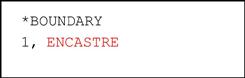
The word ENCASTRE used in the data line represents a fully built-in condition, which also means that DOFs 1 to 6 are constrained to zero. Other standard boundary conditions are listed in Table 13.2. After defining the boundary condition, we have now completed what is required for the model data of the input file.
Table 13.2
Standard boundary condition types in ABAQUS.
| Boundary Condition Type | Description |
| XSYMM | Symmetry about a plane x = constant (DOFs 1, 5, 6 = 0) |
| YSYMM | Symmetry about a plane y = constant (DOFs 2, 4, 6 = 0) |
| ZSYMM | Symmetry about a plane z = constant (DOFs 3, 4, 5 = 0) |
| ENCASTRE | Fully clamped (DOFs 1 to 6 = 0) |
| PINNED | Pinned joint (DOFs 1, 2, 3 = 0) |
| XASYMM | Antisymmetry about a plane x = constant (DOFs 2, 3, 4 = 0) |
| YASYMM | Antisymmetry about a plane y = constant (DOFs 1, 3, 5 = 0) |
| ZASYMM | Antisymmetry about a plane z = constant (DOFs 1, 2, 6 = 0) |
We would now need to define the history data. As mentioned, the history data would begin with the *STEP option. In this example, we would be required to obtain the displacements of the beam as well as the stress along the beam due to the downward force. One step would be sufficient here and the loading will be static.
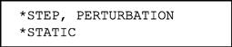
The perturbation parameter following the *STEP option basically tells ABAQUS that only a linear response should be considered. The *STATIC option specifies that a static analysis is required. The next thing to include will be the loading conditions:
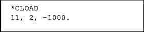
ABAQUS offers many types of loading. *CLOAD represents concentrated loading which is the case for our problem. Other types of loading include *DLOAD for distributed loading, *DFLUX for distributed thermal flux in thermal-stress analysis, *CECHARGE for concentrated electric charge for nodes of piezoelectric elements. The first entry in the data line is the node i.d. or the name of the node set, if defined, the second is the DOF the load is applied to, and the third is the value of the load. In our case, since the force is acting downward, it is acting on DOF 2 with a negative sign following the convention in ABAQUS. Most loadings can also follow an amplitude curve varying with time by including AMPLITUDE = Name of amplitude curve definition in the keyword line. This is especially so if transient, dynamic analysis is required.
For this problem, there is not much more data to include in the history data other than the output requests. The user can request the type of outputs he or she wants by indicating these as follows:
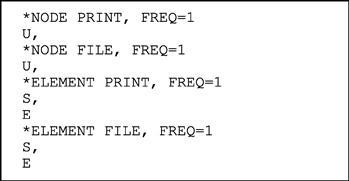
From what we learned from the finite element method, we can actually deduce that certain output variables are direct nodal variables like displacements, while others such as stress and strain, are actually determined as a distribution in the element using the shape functions. In ABAQUS, this difference is categorized into nodal output variables and element output variables. *NODE PRINT outputs the results of the required nodal variables in an ASCII text file (.dat file) while the *NODE FILE outputs the results in a binary format (.fil file). The binary format can be read by post-processors in which the results can be displayed. Similarly, *ELEMENT PRINT outputs element variables in ASCII format, while *ELEMENT FILE outputs them in binary format. A list of the different output variables can be obtained from the ABAQUS manuals. For our case, “U” in the data lines for *NODE PRINT and *NODE FILE will output all the components of the nodal displacements. “S” and “E” represent all components of stress and strain, respectively. So if the analysis is run, there will be in total three tables: One showing the nodal displacements, one showing the stresses in the elements, and the last one showing the strains in the elements. The last thing to do now is to end the step by including *ENDSTEP. If multiple steps are present, this would separate the different steps in the history data.
Running the analysis
The whole input file defining the problem of the cantilever beam is shown below:
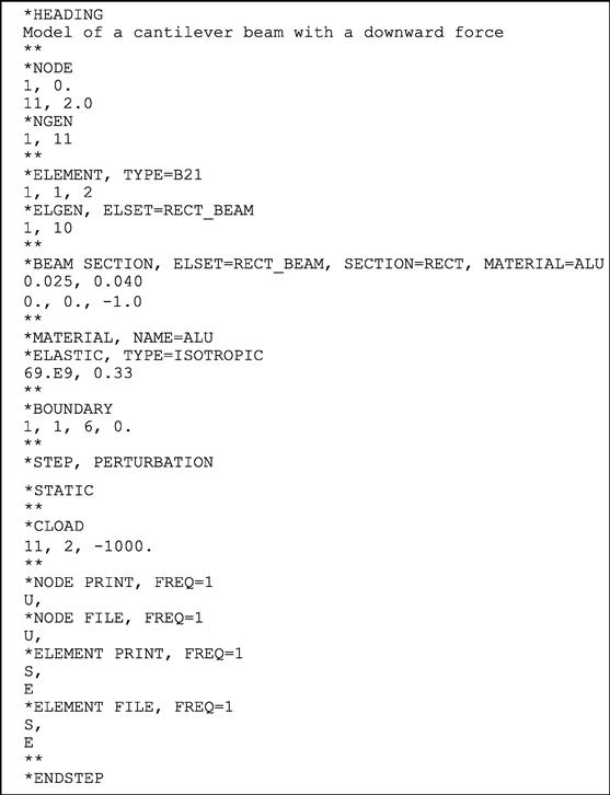
ABAQUS input files end with the extension .inp. So if we name this file as beam.inp, we can run this example in ABAQUS using the following command at the command prompt of a Linux/Unix machine:
![]()
Users can check up the full syntax of the ABAQUS execution command in the manuals (note that the execution command may vary depending on how the system administrator sets it up).
Results
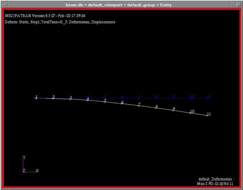
After executing the analysis, there could be several results files being generated. The beam.dat file would be in ASCII text format. ABAQUS outputs its results in ASCII format in the file ending with the extension .dat. As mentioned, the binary format would be in the file with the .fil extension and is generally used as inputs for post-processors. The .dat file can of course be viewed by any text editor and it will show lots of numbers associated with the input processing, the analysis steps and lastly the requested outputs (*NODE PRINT and *EL PRINT). These output data can of course be used for plotting graphs or as inputs to other programming codes depending on the user. Many users would view the results using post-processors like ABAQUS/CAE, PATRAN and so on. The choice is entirely up to the preference of the user and of course the availability of these post-processors. In this book, the results are viewed using PATRAN and the results are shown below.
Figure 13.3 shows the deformation plot of the cantilever beam as obtained in PATRAN. This plot shows how the cantilever beam deforms under the applied loads. The actual displacements of the nodes can also be included in the deformation plot, but if there are many nodes, it makes viewing them on screen difficult. Figure 13.4 shows an XY-plot obtained in PATRAN of the stress, σxx, on the top and bottom surface of the beam. The plot shows clearly a tensile stress on the top and a compressive stress at the bottom. XY-plots of strain and displacements can be similarly obtained in PATRAN.

13.6 General procedures
The way to write the ABAQUS input file of a simple problem of a cantilever beam has been shown in the previous section. This chapter will not go through the many keywords that are available in ABAQUS. Readers and users should consult the manuals for more information regarding the keywords. This section thus aims to provide a general guide, not just for using ABAQUS, but generally for using most finite element software.
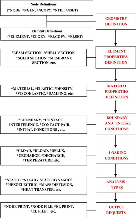
From the previous example, it is seen that certain information must be provided for the software to carry out the analysis. This information is required to solve the finite element problem, and it has been highlighted throughout this book that the information is mainly used to formulate the necessary matrices. Of course, there are certain parameters that govern the algorithm and the way the equations are solved in the program as well. So, in this sense, there should not be much difference between different software other than the format of the way information is supplied and the way results are presented. Figure 13.5 shows a summary of the general information that finite element software requires to solve most problems. The keywords provided on the left are some of the keywords used in ABAQUS to provide that particular information. To summarize, we would first need to define the geometry by defining the nodes and the elements. Remember that in the finite element method, the whole domain is discretized into small elements. This is generally called meshing. Next, we would need to provide some properties for the elements used. For example, using 1D beam elements would require one to provide the type of cross-section and the cross-section dimension; or when using 2D plate elements the thickness of the plate would be required, and so on. After that, we would need to define the properties of the material or materials being used and associated with the elements. We would then need to provide information regarding the boundary and initial conditions the model is under. This is necessary for the solver to evaluate the equations. Similarly so for the loading conditions, which must also be provided, unless there are no loads on the model, as is the case in many analyses involving natural frequencies extraction. After all this, the model is more or less defined. The next step would be to tell the software what type of problem or analysis this is. For example, is the problem a static analysis, or a transient dynamic analysis, or a heat transfer analysis? The software would require this information and the user must provide it with the analysis type. Lastly, the user can also tell the software what results he or she is seeking. For example, for most applied mechanics problems, the displacements are the true nodal variables that the solver will compute. The software, however, can also compute the stress and strain from interpolation of these nodal displacements automatically and this can be done by specifying them in the input file.
13.7 Remarks (example using a GUI: ANSYS)
The information provided in the previous sections serves to highlight the typical steps in using a finite element software package through the description of the ABAQUS input file. In practice, most FEM packages including ABAQUS (ABAQUS/CAE) provide a well-integrated user interface that allows modelers to create or input geometry; perform meshing over the geometry; prescribe the necessary material properties; impose the appropriate boundary and loading conditions; select the appropriate analysis type for the problem; perform the execution of the FEM job; and even perform post-processing and visualization of the results.
Another popular FEM software package that encompasses this idea of integrating all the procedures in a nice GUI is ANSYS. Originally developed essentially for structural mechanics and heat transfer problems, ANSYS has since been developed to offer solutions for a wide range of physical problems ranging from fluid dynamics, electromagnetics, hydrodynamics, multi-physics, and so on. This section now highlights the use of ANSYS, as an example of a typical process of creating an FEM model using a user-friendly GUI. We will repeat the earlier example of the cantilever beam using ANSYS in this section. Similar procedures can also be performed in ABAQUS/CAE.
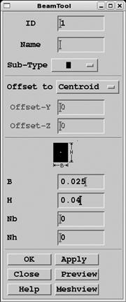
In ANSYS, one typically starts the modeling by specifying the type of elements to be used in the current model that is going to be built. Figure 13.6 shows the ANSYS environment and the dialog windows that allow one to select the appropriate element type for the problem. The figure also shows that a beam element named in ANSYS as “BEAM188” is selected. “BEAM188” is a 2-node beam in 3D space based on the Timoshenko beam theory, i.e., shear deformation is included. To model the Euler-Bernoulli beam introduced in this book (Chapter 5), one may use the “BEAM3” element, implemented via the command line. The next step after selecting the element type is to define the section properties for the beam element type. Figure 13.7 shows the pop-up window that allows one to define the section properties in ANSYS, and in it, different cross-section profiles (for the beam elements in this case) can be selected which require input of the corresponding dimensions and properties.

Typically, one then needs to provide information on the material(s) involved, and these can be prescribed in ANSYS easily via the user-friendly GUI as shown in Figure 13.8. The relevant material information is prescribed accordingly to the problem to be solved, and in this particular case, isotropic, elastic properties (Young’s modulus and Poisson ratio) are keyed in.

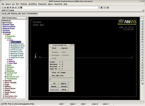
In the ANSYS environment, there are basic capabilities of geometry creation that allow modelers to create simple geometry from points, lines, and surfaces, to solids, as shown in the screen shot in Figure 13.9. In the figure, we are creating a straight line for modeling the 1D cantilever beam. For more complex geometry, ANSYS also allows the import of compatible CAD files that can be used for meshing within the software.
Recall that in the ABAQUS input file, we perform meshing of the cantilever beam structure by using the *NGEN and *ELGEN. In a GUI, the geometry is selected (in this example, a line) and appropriate mesh properties (the number of elements/nodes and/or the size of the elements) can be prescribed via the GUI as shown in Figure 13.10a. The “MeshTool” window shown in Figure 13.10b then allows one to select and mesh the geometry (in this case, the line we created).
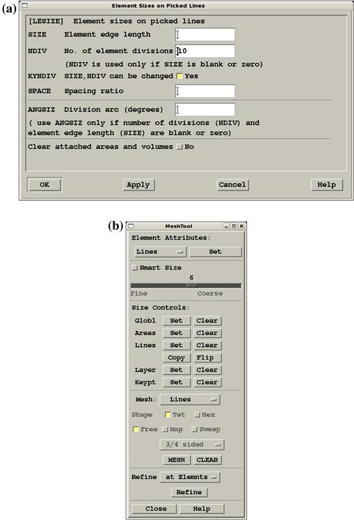
Figure 13.10 Meshing in ANSYS: (a) specifying element size and/or number of elements to be used and (b) the mesh tool window for meshing the geometry.
To prescribe the boundary and loading conditions, the geometry (e.g., surface, edge, etc.) is selected and the nodes associated with the geometry will be assigned with the boundary and loading conditions prescribed. Alternatively, the boundary and loading conditions can be applied directly to the nodes or elements by selecting them directly. Figure 13.11a shows the pop-up window for prescribing the displacement boundary conditions. In this case, “All DOF” is selected and the value of the displacement is set to “0” for the node at the clamped end of the cantilever beam. Figure 13.11b shows the window for prescribing the force. Note that the direction of the force is selected as “Fy” and “–1000” is entered as the constant value. Finally, we need to select the type of analysis to carry out. As shown in Figure 13.12, there are a variety of analyses available for selection and, in this case, “Static” analysis is chosen. Most integrated FEM packages can start the computation for the solution directly within the software GUI as shown in Figure 13.13a. Note that a summary of the model input is also shown in a separate window in the background. Once the computation is done, the results are automatically imported into the same ANSYS software environment for viewing as can be seen in Figure 13.13b.
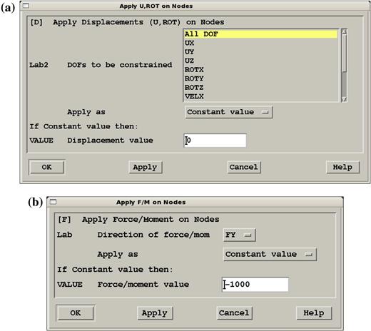
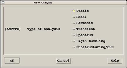
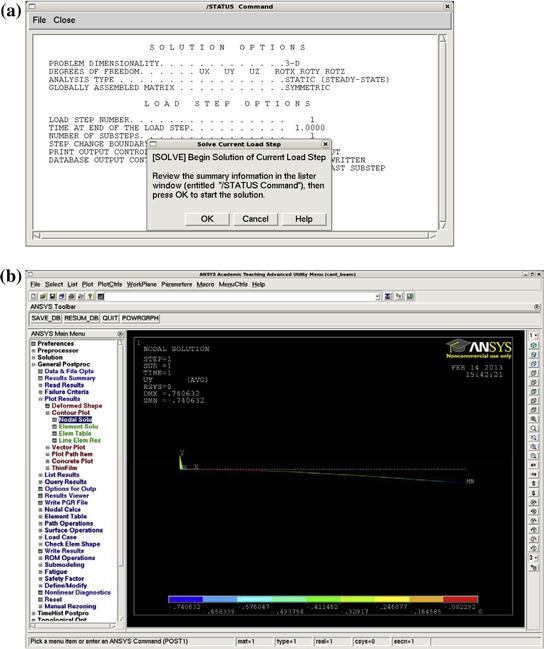
Figure 13.13 (a) The computation is started directly in the ANSYS GUI; and (b) the results can be viewed once the computation is completed.
Note that in this section, the general steps for creating and solving a simple finite element model using the GUI are highlighted via the introduction of the ANSYS software package. Our discussion is brief and is meant to provide only a rough idea of how an FEM model can be created in a commercial software package. It is of course much more sophisticated in practice, and for more details, readers are referred to the ANSYS user manual.
References
1. ABAQUS keywords manual, version 6.1: Hibbitt, Karlsson & Sorensen, Inc., 2000.
2. ABAQUS theory manual, version 6.1: Hibbitt, Karlsson & Sorenson, Inc., 2000.
3. ABAQUS user’s manual, volumes I, II, and III, version 6.1: Hibbitt, Karlsson & Sorensen, Inc., 2000.