
Modeling Techniques
11.1 Introduction
In this chapter, various modeling techniques for creating FEM models will be introduced, many of which have been discussed in NAFEMS (1986). These techniques are necessary when carrying out finite element analysis to help to ensure the reliability and accuracy of the results obtained. With the development in the power of computer hardware and software, a FEM analysis can now be performed with ease. In fact, FEM software packages are very often used as a routine tool in the design process by analysts who may not have a proper background of finite element analysis. To many analysts, the FEM software is like a “black box,” into which inputs are prescribed, and out of which results are computed and visualized. However, it should be stressed that improper use of commercial software can lead to erroneous results, which are often obscured by colorful stress or deformation plots, movies or other post-processed results. The earlier chapters of this book aim to imbue readers with a clear idea of what goes on in a commercial FE software package. The primary objective of this chapter is to present practical modeling techniques that ensure proper implementations of the FEM theory, and to avoid unnecessary mistakes in creating a FEM model when using a commercial package.
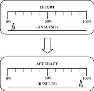
Another reason to learn some of these modeling techniques is to improve both the efficiency of the computation as well as the accuracy of the results. An experienced analyst should be able to obtain accurate results with as little effort in modeling and using as little computer resources as possible. The efficiency of the FE analysis is measured by the effort to accuracy ratio as shown in Figure 11.1. For example, the use of a symmetrical model to simulate a problem with symmetrical geometry can greatly reduce the modeling and computation time with possibly even more accurate numerical results. Therefore, a good FEM model requires more than just discretizing the problem domain with elements. To come up with a good finite element model, the following factors need to be considered:
11.2 CPU time estimation
Despite continuous advances in the computer industry, computer resource can still be one of the decisive factors limiting how complex a finite element model can be built. The CPU time required for a static analysis can be roughly estimated using the following simple relation (it is termed as complexity of a linear algebraic system):
![]() (11.1)
(11.1)
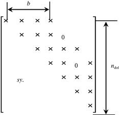
where ndof is the number of the total degrees of freedom (DOFs) in the finite element equation system, and α is a constant that is in general in the range of 1.7 to 3.0 depending on different solvers used in the FEM package and the structure of the stiffness matrix.
One of the very important factors that affect α is the bandwidth of the stiffness matrix as illustrated in Figure 11.2. The smaller the bandwidth the smaller the value of α, and hence a faster computation. From the direct assembly procedure described in Example 4.2, it is clear that bandwidth depends on the difference of the global node number assigned to the elements. The element that has the biggest difference in node number controls is the bandwidth of the global stiffness matrix. The bandwidth can be changed even for the same FEM model by changing the global numbering of the nodes. Therefore, tools have been developed for minimizing the bandwidth through re-numbering of nodes. Most of the FEM packages have one or more of such tools built-in. The user can simply invoke the tool in the FEM software to minimize the bandwidth after meshing the problem domain. This simple operation can sometimes reduce the CPU time drastically. A very simple method for minimizing the difference of node numbers and hence the bandwidth can be found in the book by Liu (2009, Chapter 15).
Equation (11.1) clearly indicates that a finer mesh, with a large number of DOFs, results in an exponentially increasing computational time. This implies the importance of the reduction of the DOFs. Many techniques discussed in this chapter are related to the reduction of DOFs. Our aims are therefore:
1. To create a FEM model with minimum DOFs by using elements of as low a dimension as possible, and
2. To use as coarse a mesh as possible, and use fine meshes only for important areas.
These have to be done without sacrificing the desired accuracy of the results.
11.3 Geometry modeling
Actual physical structures are usually very complex. The analyst should decide on the ways, where possible, to reduce a complex geometry to a manageable one. The first issue the analyst needs to consider is the type of elements that should be used: 3D elements? 2D (2D solids, plates, and shells) elements? Or 1D (truss and beam) elements? This requires a good understanding of the mechanics of the problem and the behavior of the structure. As we have mentioned in Chapter 9, 3D elements can be used for modeling all types of structures. However, it can be extremely expensive if 3D elements are used everywhere in the entire problem domain, because it will definitely lead to a huge number of DOFs. Therefore, for complex problems, the mesh is often a combination of different types of elements created by taking full geometrical advantage of the problem domain. The analyst should analyze the problem in hand, examine the geometry of the problem domain, and try to make use of 2D and 1D elements for areas or parts of the structure that satisfy the assumptions that lead to the formulation of 2D or 1D elements. Usually, 2D elements should be used for areas/parts that have a plate- or shell-like geometry, and 1D elements should be used for areas/parts that have a bar- or arch-like geometry. 3D elements are used only for bulky parts of the structure to which 2D or 1D elements cannot apply. This process is very important because the use of 2D and 1D elements can significantly reduce the number of DOFs.
As shown in Figure 11.3, for the modeling of parts where 3D elements are to be used, 3D objects that have the same geometrical shapes of the structure have to be created. For parts where 2D elements are to be used, only the neutral surfaces that are often the geometrical mid-surfaces need to be created. For parts where 1D elements are to be used, only the neutral axes that are often the geometrical mid-axes need to be created. Therefore, one can imagine that by using 2D and 1D elements, the task of creating the geometry is significantly simplified.

Figure 11.3 Geometrical modeling. (a) Physical geometry of the structural parts; (b) Geometry created in FEM models.
When a mix of different types of elements are used in an FEM model, the interfaces where the different element types meet requires additional attention. At these interfaces, techniques of modeling joints can be used, which will be discussed in detail in Section 11.9. These techniques are required because the type of DOFs at a node that is shared by different element types is different for different element types. Recall that the DOFs for any particular element type arise from the theories of mechanics discussed in Chapter 2 and depends on the mechanics of the problem (e.g., truss, beam, 2D solids, plate, etc.). Table 11.1 lists the number of DOFs for some different types of elements.
Table 11.1
Type of elements and number of DOFs at a node.
| No. | Description | DOFs at a Node |
| 1 | 2D frame analysis (using 2D frame element) | 3 (2 translations and 1 rotation) |
| 2 | 3D frame analysis (using 3D frame element) | 6 (3 translations and 3 rotations) |
| 3 | 2D analysis for plane strain or plane stress analysis | 2 (translational displacements) |
| 4 | 3D analysis for solids with general geometries and loading conditions | 3 (translational displacements) |
| 5 | 2D analysis for axisymmetric solids with axisymmetric or asymmetric loading | 2 (translational displacements) |
| 6 | Plate bending analysis for out-of-plane loading (bending effects only) | 3 (1 translation and 2 rotations) |
| 7 | General plate and assembled plate analysis with general loading conditions (combined membrane and bending effects) | 5 or 6 (3 translations and 2 or 3 rotations) |
| 8 | General shell analysis for shell structures (coupled membrane and bending effects) | 5 (or 6) (3 translations and 2 or 3 rotations) |
| 9 | 1D analysis for axisymmetric shells with axisymmetric loading (membrane and bending effects) | 3 (2 translations and 1 rotation) |
Understanding the requirements needed for the analysis is important and has a direct bearing on the generation of the simulation domain. For example, analysts will usually give a detailed modeling of the geometry for areas where critical results are expected. Note that many structures are now designed using so-called computer aided design (CAD) packages. Therefore, the geometry of the structure would have already been created electronically. Most commercial pre-processors of FEM software packages can read CAD files in certain formats. Making use of these CAD files can reduce the effort in creating the geometry of the structure, but it requires a certain amount of effort to modify the CAD geometry for them to be suitable for FEM meshing. There are also ongoing research activities to automatically convert proper 3D geometries to 2D and 1D geometries for FEM mesh, but at the time of writing, such tools have not matured sufficiently for commercial applications.
11.4 Meshing
11.4.1 Mesh density
To minimize the DOFs, it is common to create a mesh of varying density. We usually only need a fine mesh in areas of importance, such as areas of analytical interest, and expected zones of stress concentration, such as at re-entrant corners; holes; slots; notches; or cracks. An example of a finite element mesh exhibiting mesh density transition is shown in Figure 11.4. In this example of the sprocket-chain system of a motorcycle, the focus of the analysis is the contact forces between the sprocket and the chain. Hence, the region at the center of the sprocket is relatively less critical and the mesh used at that region is therefore coarser.
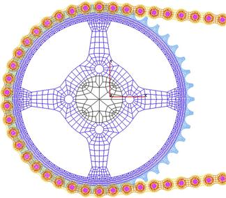
Figure 11.4 Finite element mesh for a sprocket-chain system. (Courtesy of the Institute of High Performance Computing.)
In using FEM packages, the control of mesh density is often performed by creating what are commonly termed “mesh seeds.” Mesh seeds are placed on a given or created geometry before actual meshing. These mesh seeds indicate the positions of the nodes of the actual finite element mesh where the node density needs to be controlled. To have more elements in areas of importance, denser mesh seeds are simply placed in these areas before meshing. When the mesh is being generated, nodes will be created at the locations of these seeds.
11.4.2 Element distortion
It is not always possible to fit regularly shaped elements into irregular geometries. Irregular or distorted elements are acceptable in FEM, but there are limitations and one needs to control the degree of element distortion in the process of mesh generation. The element distortions are measured against the basic shape of the element which are:
Five possible forms of element distortions and their rule-of-thumb limits are listed as follows:
1. Aspect ratio distortion (elongation of element) as shown in Figure 11.5.
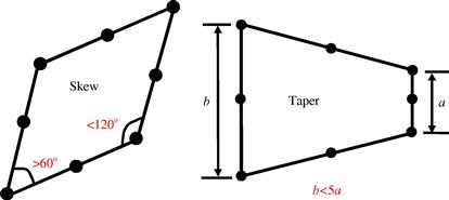
2. Angular distortion of the element (Figure 11.6), where any included angle between edges approaches either 0° or 180° (skew and taper).
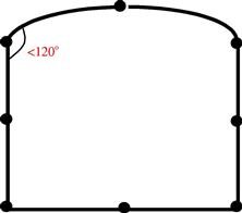
3. Curvature distortion of element (Figure 11.7), where the straight edges from an element are distorted into curves when matching the nodes to the geometric points.
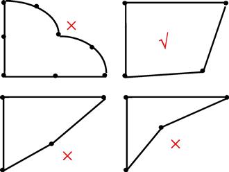
Volumetric distortion occurs in concave elements. As discussed in Chapter 6, in calculating the element stiffness matrix, a mapping is performed to transfer the irregular shape of the element in the physical coordinate system into a regular one in the non-dimensional natural coordinate system. For concave elements, there are areas outside the elements (see the shadowed area in Figure 11.8) that will be transformed into an internal area in the natural coordinate system. The element volume integration for the shadowed area based on the natural coordinate system will thus result in a negative value. A few unacceptable shapes of quadrilateral elements are shown in Figure 11.9.

Figure 11.8 Mapping between the physical coordinate (x − y) and the natural coordinate (ξ − η) for a heavily volumetrically distorted elements leads to mapping of an area outside of the physical element into an interior area in the natural coordinates.
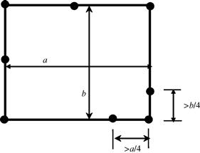
Mid-node position distortion occurs with higher order elements where there are mid-nodes. The mid-node should be placed as close as possible to the middle of the element edge. The limit for mid-node displacing away from the middle edge of the element is a quarter of the element edge, as shown in Figure 11.10. The reason behind this is that shifting of mid-nodes can result in undesirable stress distribution and even singular stress field in the elements as discussed in Section 10.2.
Many pre-processors of the FEM package provide a tool for analyzing the element distortion rate for a created mesh. It is good practice prior to submitting a finite element model for computation to invoke this built-in tool to check for element distortion. A report of distortion rates will be generated for the analyst’s examination or heavily distorted elements can be highlighted for any necessary actions.
11.5 Mesh compatibility
In Chapter 3, when the Hamilton’s principle is used for deriving the FEM equation, it is required that the displacement has to be admissible, which demands the continuity of the displacement field in the entire problem domain. A mesh is said to be compatible if the displacements are continuous along all the edges between all the elements in the mesh. The use of different types of elements in the same mesh or improper connection of elements can result in an incompatible mesh. The following two subsections will discuss the reasons for mesh incompatibility and suggest methods for fixing or avoiding mesh incompatibility issues. Note that the compatibility conditions can be relaxed if the S-PIM (Liu and Zhang, 2013) is used. This is because the S-PIM is based on the so-called weakened weak form, and the stability and convergence are ensured by the G-space theory.
11.5.1 Different order of elements
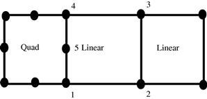
Mesh incompatibility issues can arise when we have a transition between different mesh densities or when we have meshes comprising of different element types. When a quadratic element is joined with one or more linear elements as shown in Figure 11.11, incompatibility arises due to the difference in the orders of shape functions used. The 8-nodal quadratic element in Figure 11.11 has quadratic shape functions, which implies that the deformation along the edge follows a quadratic function. On the other hand, the linear shape function used in the 4-nodal linear element in Figure 11.11 will result in a linear deformation along each element edge. For the case shown in Figure 11.11a, the displacements at nodes 1 and 3 for the quadratic element and the linear elements are the same, but deformation of the edges between nodes 1 and 3 will be different. Assuming that nodes 1 and 2 have zero displacements, while node 3 gets displaced, the deformations of these edges can then be shown by the dotted lines in Figure 11.11. A crack-like behavior is clearly observed which can lead to severe erroneous results. For the case shown in Figure 11.11b, the displacements at nodes 1, 2 and 3 for the quadratic element and the two linear elements are the same, but the deformation of the edges between nodes 1 and 2, and nodes 2 and 3 will again be different. If nodes 1 and 3 have zero displacements, while node 2 gets displaced, the deformations of these edges are shown by the dotted lines in Figure 11.11. Again, a crack-like behavior is clearly observed.

Figure 11.11 Incompatible mesh caused by the different shape functions along the common edge of the quadratic and linear elements. (a) A quadratic element connected to one linear element. (b) A quadratic element connected to two linear elements.
Here are some solutions to avoid or solve these mesh incompatibility issues:
1. Use the same type of elements throughout the entire problem domain. This is the simplest solution and is a usual practice, as complete compatibility is automatically satisfied if the same elements are used as those shown in Figure 11.12.
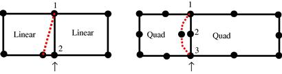
Figure 11.12 Use of elements of the same type with complete edge to edge connection automatically ensures the mesh compatibility.
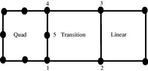
2. When elements of different orders of shape functions have to be used for some reason, such as in p-adaptive analysis, use transition elements whose shape functions have different orders on different edges. An example of a transition element is shown in Figure 11.13. The 5-node element shown can behave in a quadratic fashion on the left edge and linearly on the other edges. In this way, the compatibility of the mesh can be guaranteed.
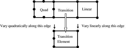
Figure 11.13 A transition element with 5 nodes used to connect linear and quadratic elements to ensure mesh compatibility.
3. Another method used to enforce mesh compatibility is to use multipoint constraints (MPC) equations. MPCs can be used to enforce compatibility for cases shown in Figure 11.11a. This method is more complicated, and requires the knowledge of creating MPC equations, which will be covered in Section 11.10.
11.5.2 Straddling elements
Straddling elements can also result in mesh incompatibility as illustrated in Figure 11.14. Although the order of the shape functions of these connected elements are the same, the straddling can result in an incompatible deformation of edges between nodes 1 and 2, and 2 and 3, as indicated by the dotted lines in Figure 11.14. This is because in the assembly of elements, the FEM requires only the continuity of the displacements (not the derivatives) at nodes between elements.

Figure 11.14 Incompatible mesh caused by the straddling along the common edge of the same order of elements.
The solution to this problem is simply to make sure there are no straddling elements in the mesh. Most mesh generators are designed not to produce such an element in the mesh. However, care needs to be taken if the mesh is created manually.
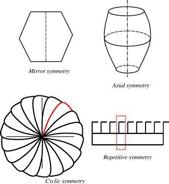
11.6 Use of symmetry
Many structures and objects exhibit some form of symmetry. Figure 11.15 shows some examples of the different types of common structural symmetry. Objects such as a can of drink exhibits axial symmetry and even huge structures such as the Eiffel Tower of Paris exhibits mirror symmetry. An experienced analyst will take full advantage of such symmetries in structures to simplify their modeling process as well as to reduce the DOFs and hence computational time required for the analysis. Imagine a full finite element model of the Eiffel Tower consisting of, say, 100,000 elements. Because of the mirror symmetry, one can actually perform the analysis by just modeling a quarter of the whole structure and the number of elements will be reduced to a quarter at 25,000 elements. The total DOFs of the system will also be reduced to a quarter. Using Eq. (11.1) and assuming that α = 3, it can be found that the CPU time will be reduced to (1/4)3 = (1/64)th of that required for solving the full model. The significance is astonishing! Furthermore, since only a quarter of the model is required, the time for the analyst to create the model is also reduced. In addition, the accuracy of the analysis can be improved as the equation system becomes much smaller and the numerical errors in the computation will reduce. However, proper techniques have to be used to make the full use of the structural symmetry. This section will deal with some of these techniques.
11.6.1 Mirror symmetry or plane symmetry
Mirror symmetry is the symmetry about a particular plane, and it is the most prevailing case of symmetry. A half of the structure is the mirror image of another. The position of the mirror is called the plane of symmetry. A structure is said to have mirror structural symmetry if there is symmetry of geometry, support conditions, and material properties. Many actual structures exhibit this type of symmetry. Some of these structures are actually symmetrical about a particular plane, while others are symmetric with respect to multiple planes. Take for example a cubic block as shown in Figure 11.16. One can actually use the property of single-plane-symmetry and model a half-model or one can use that of two-plane-symmetry to further reduce the finite element model to a quarter of the original structure. In fact, more planes of symmetry can also be used to just model one-eighth of the model and in that case, it would be similar to the case of cyclic symmetry, which will be discussed later.

Consider a symmetric 2D solid shown in Figure 11.17. The 2D solid is symmetric with respect to an axis of symmetry of x = c. The left half of the domain is modeled with impositions of the following symmetric boundary conditions at nodes on the symmetric axis.
 (11.2)
where ui (i = 1,2,3) denotes the displacements in the x direction at node i. Equation (11.2) gives a set of single point constraint (SPC) equations, because in each equation, there is only one unknown (or one DOF) involved. This kind of SPC can be simply imposed by removing the corresponding row and column in the global system equations as demonstrated in Examples 4.1 and 4.2.
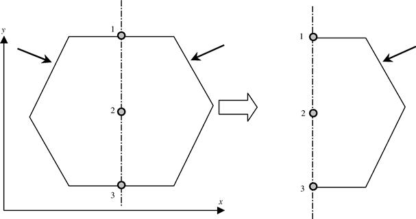
Figure 11.17 2D solid with an axis of symmetry at x = c. The right half of the domain is modeled with impositions of symmetric boundary conditions at nodes on the symmetric axis.
Loading conditions on a symmetrical structure must also be taken into consideration. A loading is considered symmetric if the loading can also be “reflected” off a particular plane as shown in Figure 11.18. In this case, the problem is symmetric because the whole structure, its support conditions, as well as its loading, is symmetrical about the plane x = 0. An analysis of a half of the whole beam structure using the symmetrical boundary condition at x = 0 would yield a complete solution as that of the full model with at least less than a quarter of the effort.
A problem can also be anti-symmetric, if the structure is symmetric but the loading is anti-symmetric, as shown in Figure 11.19. Again, modeling half of the structure can also yield a complete solution using an anti-symmetric boundary condition, which would be different on the plane of symmetry. In the simple example shown in Figure 11.19, the anti-symmetric boundary condition is that the deformation at the plane of symmetry should be zero. Note that the rotation at the plane of symmetry need not be zero in contrast with the case of symmetric loading.

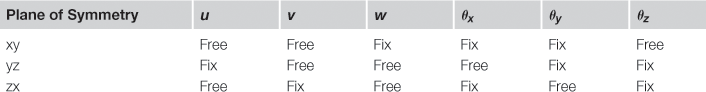
The following general rules can be applied when deciding the boundary conditions at the plane of symmetry. If the problem is symmetric as shown in Figure 11.18, then:
1. There are no translational displacement components normal to the plane of symmetry.
2. There are no rotational displacement components with respect to the axis that are parallel to the plane of symmetry.
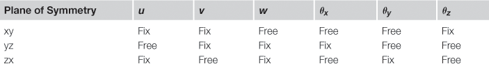
If the problem is anti-symmetric as shown in Figure 11.19, then:
1. There are no translational displacement components parallel to the plane of symmetry.
2. There are no rotational displacement components with respect to the axis that is normal to the plane of symmetry.
Tables 11.2 and 11.3 give the complete list of conditions for symmetry and anti-symmetry for general three-dimensional cases.
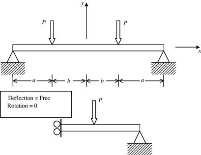
Any load can be decomposed into a symmetric load and an anti-symmetric load. Therefore, as long as the structure is symmetric (in geometry, material, and boundary conditions), one can always take advantage of the symmetry. Consider now a case shown in Figure 11.20a where the simply supported beam structure is symmetric structurally but the loading is asymmetric (neither symmetric nor anti-symmetric). The structure can always be treated as a combination of (a) the same structure with symmetric loading and (b) the same structure with anti-symmetric loading. In this case, one needs to solve two problems with each problem having half the number of DOFs if the whole structure is modeled. One of the problems is symmetrical while the other is anti-symmetric.

Figure 11.20 Simply supported symmetric beam structure subject to an asymmetric load. (a) A structure with an asymmetric load. (b) The same structure with symmetric load. (c) The same structure with anti-symmetric load.
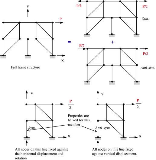
Figure 11.21 shows a more complex example of how a framework with asymmetric loading conditions can be analyzed using a half of the framework with symmetric and anti-symmetric conditions. Adding up one problem of the same structure subjected to a symmetric loading with another of the same structure subject to anti-symmetric loading is equivalent to that of analyzing the full frame structure with the asymmetric loading. In this example, there is actually a frame member that is at the plane of symmetry. The properties of this frame member on the symmetric plane need to be halved as well for the two half models. This means that all the properties that contribute to the stiffness matrix for this member need to be halved.
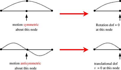
Dynamic problems can also be solved in a similar manner using the symmetric or anti-symmetric properties, for example, if symmetric boundary conditions are imposed on a simple beam structure and a natural frequency analysis is carried out. The natural frequencies obtained will correspond only to the symmetrical modes. To obtain the anti-symmetrical modes, anti-symmetrical boundary conditions will need to be applied to the model. Figure 11.22 shows the symmetric and anti-symmetric conditions for vibration analysis in a simply supported beam.
11.6.2 Axial symmetry
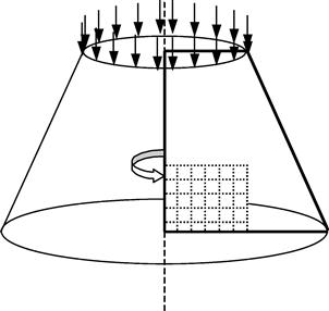
A solid or structure has axial symmetry when it can be generated by rotating a planar geometry (1D or 2D) about an axis. To take advantage of axial symmetry, such a solid can be modeled by simply using 1D or 2D axisymmetric elements, as discussed in Chapter 7. In doing so, there is a dimension reduction that will greatly reduce the modeling and computational effort. For example, a cylindrical shell structure can be modeled using 1D axisymmetric beam elements as shown in Figure 11.23. Figure 11.24 shows an example of a 3D solid under axially symmetric loads, which can be modeled using 2D axisymmetric elements.

The formulation of 2D axisymmetric elements is detailed in Section 7.5 and it has been shown that it is very similar to the formulation of 2D plane strain elements. Similarly, the formulation of 1D axisymmetric elements can be easily developed using similar concepts to those used in earlier chapters, but expressed in the polar coordinate system. The shapes for 2D axisymmetric elements are the same as that of regular 2D elements described in Chapter 7. Generally speaking, the use of axisymmetric elements requires much less computational resources compared to a full 3D discretization. Axisymmetric elements are readily available in most finite element software packages, and the usage of these elements is similar to the regular 1D or 2D elements.
Similar to the plane symmetry problems, the loadings applied on an axisymmetric structure do not have to be symmetric or anti-symmetric about its axis. Any axially asymmetric load can be expressed in a Fourier superimposition of both axial symmetric and axial anti-symmetric components in the θ direction. Therefore, the problem can always be decomposed into two sets of problems of axial symmetric and axial anti-symmetric, as long as the structure is axisymmetric (in geometry, material and boundary support).
11.6.3 Cyclic symmetry
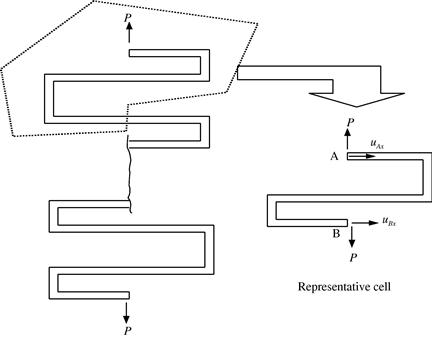
Cyclic symmetry exists in problems whereby both geometry and loading appear as repeated sectors in a cyclic manner. In such a case, a complete solution can be obtained by analyzing only one sector as a representative cell with a set of cyclic boundary conditions on the boundaries of the cell, as shown in Figure 11.25. The cyclic symmetric boundary condition for the problem shown in Figure 11.25 requires that all the variables along side A must match exactly those on side B. Constraint equations at all the corresponding nodes along side A and side B can therefore be written as
![]() (11.3)
(11.3)
![]() (11.4)
(11.4)

Figure 11.25 Representative cell isolated from a cyclic symmetric structure and the cyclic symmetrical conditions on the cell.
Note that in Eqs. (11.3) and (11.4) both uAn and uBn (or uAt and uBt) are unknowns. Thus, Eqs. (11.3) and (11.4) are constraint equations that involve more than one DOF in one equation. These types of constraint equations are termed as Multiple Point Constraints (MPC) equations, which have to be imposed by modifying the global system equations. The imposition of MPCs is, however, more tedious than that of SPC detailed in Chapter 4. To impose an SPC all one needs to do is to remove (or modify) the corresponding row and column in the system equations (see Examples 4.1 and 4.2). The imposition of a MPC requires the use of either penalty method or the method of Lagrange multipliers that will be detailed in Section 11.11.
11.6.4 Repetitive symmetry
Repetitive symmetry exists in structures consisting of continuously repeating sections under certain loading conditions (usually in the direction of repeating section), as shown in Figure 11.26. In such a case, only one section needs to be modeled and analyzed. Similar to cyclic symmetry, constraint equations are used for the corresponding nodes at the sectioned surface such that
![]() (11.5)
(11.5)
which is again an MPC equation.
11.7 Modeling of offsets
11.7.1 Methods for modeling offsets
In the modeling of beams, plates, and shells, the elements are usually defined on the neutral surface (often the geometric middle surface) of the structure, as shown in Figure 11.3. For elements that are not collinear or coplanar, there will be a distance of offset between the nodes in the FEM mode, which are connected together in the physical structure. Figure 11.27 shows a typical case of two beams with different thicknesses joined at the corner. In the finite element mesh, the two corner nodes are, however, apart. In this case, there are two offsets, α and β. In such cases, proper techniques may be needed to model the offset in order to better represent the connection.
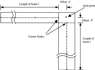
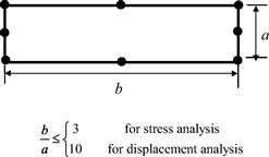
If the offsets are small compared to the length of the beam l, we can often ignore them and the connection is simply modeled by extending the corner nodes to the joint point (see Figure 11.27). If the offsets are too large, they have to be treated using proper modeling techniques. Whether offsets should be modeled depends on the engineering judgment of the analyst. A rough guideline shown below can be followed where l is the length of the beam:
![]() , offset may need to be modeled
, offset may need to be modeled
![]() , ordinary beam, plate, and shell elements may not be used. Use 2D or 3D solid elements instead.
, ordinary beam, plate, and shell elements may not be used. Use 2D or 3D solid elements instead.
Modeling of offsets is usually even more crucial in shells as there are both in-plane and out-of-plane forces in the formulation, and a small variation of nodal distance can give rise to a significant difference in results. There are three methods often used to model the offsets:
1. Very stiff element. Use an artificial element with very high stiffness (high Young’s modulus, large cross-sectional area or second moment of area) to connect the two corner nodes (see Figure 11.28a). This is usually done by increasing the Young’s modulus by, say, 106 times for the very stiff element. This method is very simple and convenient to use, but is usually not recommended because of the huge difference in stiffness between the stiff element and the normal elements in the same FE model that can lead to ill conditioning of the final global stiffness matrix.
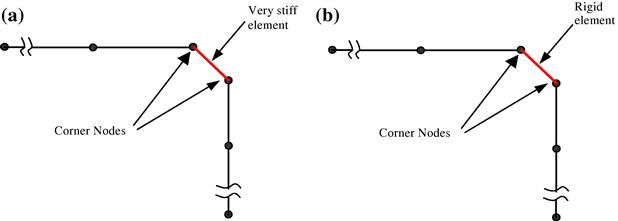
Figure 11.28 Modeling of offsets using an artificial element connecting the two corner nodes. (a) Use of very stiff element. (b) Use of rigid element.
2. Rigid element. Use a “rigid element” to connect the corner nodes (see Figure 11.29b). This method can be easily implemented being available in many commercial software packages, and all the analyst needs to do is to create an element in between the two corner nodes and then assign it as a “rigid element.” The treatment of the rigid element in the software package is the same as the next method of using MPC equations, but the formulation and implementation is automated in the software package, and therefore the user does not have to formulate these MPC equations.

Figure 11.29 Modeling of offsets using MPC equations created using a virtual “rigid body” connecting two corner nodes.
3. MPC equations. If the “rigid element” is not available in the software package, we then need to create MPC equations to establish the relationship between the DOFs at the two corner nodes. This set of MPC equations is then prescribed as an input in the pre-processor. Use of MPC equations is supported by most FEM software packages. To establish the MPC equations, we can consider a virtual rigid body that connects these two corner nodes, as shown in Figure 11.29. The detailed process is discussed in the next subsection.
11.7.2 Creation of MPC equations for offsets
The basic idea of using MPC is to create a set of MPC equations that gives the relation between the DOFs of the two separated nodes, i.e., the DOFs of one node depend on the other and vice versa. We first assume that a rigid body connects the two corner nodes. Note that this rigid body is imaginary and is used here to help us establish the MPC equations. The MPC equations are then derived using the simple kinematic relations of the DOFs on the rigid body. The procedure of deriving the MPC equations for this case of Figure 11.30 is described as follows.

First, assume that nodes 1 and 2 are perfectly connected to the rigid body and that the rigid body has a movement of q1, q2 (horizontal and vertical translations), and q3 (rotation) with reference to point 3, as shown in Figure 11.30. Then, enforce points 1 and 2 to follow the rigid body movement, and calculate the resultant displacements at nodes 1 and 2 in terms of q1, q2, and q3 to obtain
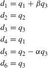 (11.6)
Finally, eliminating the DOFs for the rigid body q1, q2, and q3 from the above six equations, we obtain three MPC equations:
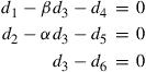 (11.7)
which gives the relationship between the six DOFs at nodes 1 and 2. Note that small displacements and rotations are assumed when deriving Eq. (11.6).
The number of the MPC equations one should have can be determined with the following equation:
![]() (11.8)
(11.8)
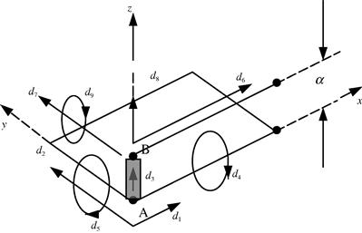
Another example of an offset often seen in engineering structures is the stiffened plates or shells, where a beam is fixed to a plate or shell as a stiffener, as shown in Figure 11.31. For the analysis of such a structural component, offset should be modeled if accurate results are required. The offset can be modeled by imagining that the node on the beam is connected to the corresponding node at the plate by a rigid body A-B. For a node in the plate, there are five DOFs (three translational and two rotational about the two axes in the plane of the plate), as shown in Figure 11.32. For a node in the beam, there are four DOFs (three translational and one rotational about the axis perpendicular to the bending plane). Note that in this case, the beam has been defined with its bending plane as the x-z plane. Hence, there are a total of nine DOFs linked by the rigid body between the node on the beam and the node on the plate. To simplify the process of deriving MPC equations, we let the rigid body follow the movement of node A in the plate. Therefore, the rigid body should have the same number of DOFs as the node in the plate, which is five: q1, q2, q3, q4 and q5. The number of MPC equations should therefore be 9 − 5 = 4 following Eq. (11.8). As the rigid body follows the movement of A in the plate, what should be done is to force the node belonging to the beam to follow the movement of B on the rigid body. We can write down the 9 DOFs of the nodes involved in terms of q1 to q5, then eliminate the five q’s from the nine equations. The resulting four constraint equations should therefore be
 (11.9)
The above equations must be specified as constraints for all the pairs of nodes along the length of the beam attached to the plate. This ensures that the beam is perfectly attached to the plate.

11.8 Modeling of supports
Support of a structure is usually very complex and in real physical structures, can be ambiguous. The FEM allows constraints to be imposed differently at different nodes. Different methods can be used to simulate these supports. For example, in the analysis of thick beam structures using 2D plane stress elements, there are three possible ways to model the support conditions at the built-in end, as shown in Figure 11.33.
1. Full constraint is imposed at the boundary nodes only in the horizontal direction.
2. Partial full constraint to the nodes on the boundary.
3. Fully clamped boundary conditions are specified at all the boundary nodes.

It is not possible to say which is the best boundary condition for the support, because the best way is actually the one that best simulates the actual situation. Therefore, good engineering judgment, experience, and the understanding of the actual support play very important roles in creating a suitable boundary condition for the finite element model. Trial and error, parametric studies, and even inverse analysis (Liu and Han, 2003) are often conducted when the physical situation is not clear to the analyst. Similarly for a prop support of a beam, there can be more than one way of modeling the support conditions as shown in Figure 11.34.

For complex support on structures, it might be necessary to use finer meshes near the boundary. Denser nodes provide more flexibility to model the support, as the FEM allows the specification of different constraints at different nodes.
11.9 Modeling of joints
Care should be taken if the joints are between different element types. The complication comes from the difference in DOFs at a node shared by different elements. In many situations, a proper technique or a set of MPC equations are required to model the connection.
Consider a connection between the turbine blade and the turbine disc shown in Figure 11.35a. A turbine blade is usually perfectly connected to a disc. The task at hand is to build a FEM model to analyze the blade-disc system. If both the blade and disc are all modeled using 2D solid elements, as shown in Figure 11.35b, perfect connection is ensured, as long as we ensure that at the interface the blade and the disc share the same nodes, i.e., there is no more than one node at any particular location.

Figure 11.35 Modeling of turbine-blade and turbine-disc system. (a) Simplified diagram of a turbine blade connected to a turbine disc. (b) A magnified 2D solid element mesh in at the interface.
Assume a FEM model where the blade is now modeled using beam elements, and the disc is modeled using 2D elements as shown in Figure 11.36. This model clearly reduces the number of nodes and therefore the DOFs. However, one needs to exercise caution when modeling the connection properly for the following reason.
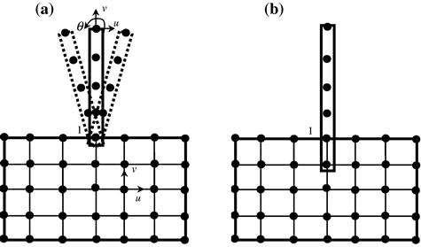
Figure 11.36 Joint between beam and 2D elements. (a) Beam is free to rotate in reference to the 2D solid. (b) Perfect connections are modeled by artificially extending beam into 2D element mesh.
First, we consider the connection of the beam element and 2D solid elements in the way shown in Figure 11.36a. From Table 11.1, we know that at a node in a 2D solid element, there are 2 DOFs: translational displacement components u and v. At a node in a beam element, there should be 3 DOFs: 2 translational displacement components u and v, and one rotational DOF. Although the beam element and the 2D elements share the common node 1, which ensures that the translational displacements are the same at the connection point for the beam and 2D solid elements, the rotation DOF of the beam element is, however, free. Therefore, the extra DOF can cause the blade to rotate freely since it is not tied (but pinned) to the 2D solid, which is not the perfect connection we wanted to model. The case here is similar to a beam with a pinned support at one end, wherein the rotational DOF is free. The problem, as you may have noticed, is due to the mismatch of the types of DOFs between the beam and 2D solid elements. The rotational DOF cannot be transmitted onto the node on a 2D solid element node, simply because it does not have a rotational DOF. We therefore require certain modeling techniques to correct this connection between the turbine blade and disc.
A simple method to fix the rotation of the beam on the 2D solid mesh is to extend the beam elements into the disc for at least two nodes, as shown in Figure 11.36b. Burying the nodes of the beam elements into the 2D mesh this way transmits the physical rotation of the beam via the translational DOFs. One may notice that the rotation of the beam at the interface is no longer free like in a pinned connection. The drawback of this simple method, however, is the additional mass introduced near the joint area due to the extension into the 2D mesh, which may affect the results of a dynamic analysis.
Another effective approach is to use MPC equations to create a connection between the two types of elements. The detailed process is given as follows.
First, imagine now that there is a very thin rigid strip connecting the beam and the disc, as shown in Figure 11.37. This strip connects three nodes together, one on the beam and two on the disc. These three nodes have to move together with the rigid strip. The MPC equations can then be established in a similar manner as that discussed for offsets.

Figure 11.37 Modeling of the turbine blade connected to the disc using a rigid strip to create MPC equations.
Note that a node on the beam has three DOFs whereas the two nodes on the disc have a total of four DOFs. The total DOFs connected to the rigid strip is thus seven. Since the DOF of the rigid strip is three, we should have four MPC equations based on Eq. (11.8). The four MPC equations, after eliminating the rigid DOFs, are given as follows:
 (11.10)
These equations enforce full compatibility between the beam and the disc.
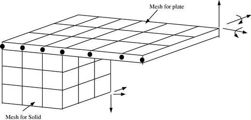
A similar problem arises when plate or shell elements that possess rotational DOFs are connected to 3D solid elements that do not possess a rotational DOF. Such a connection between a plate and a 3D solid, as shown in Figure 11.38, can be similarly modeled using the above methods.
11.10 Other applications of MPC equations
11.10.1 Modeling of symmetric boundary conditions
When discussing the modeling of symmetric problems, it was mentioned that constraint (boundary) equations are required to ensure that symmetry is properly defined. Note that Eq. (11.2) was obtained when the axis or plane of symmetry is parallel (or perpendicular) to an axis of the Cartesian coordinates. When the axis or plane of symmetry is not parallel (or perpendicular) to x or y axis, as shown in Figure 11.39, the displacement in the normal direction of the axis or plane of symmetry should be zero, i.e.,
![]() (11.11)
(11.11)
![]() (11.12)
(11.12)
where ui and vi denote the x and y components of displacement at node i. Equation (11.12) is an MPC equation, as it involves more than one DOF (ui and vi). When α = 0, the axis of symmetry is parallel to y axis, and Eq. (11.12) will reduce to an SPC as in Eq. (11.2).

11.10.2 Enforcement of mesh compatibility
Section 11.5.1 discussed mesh compatibility issues and it was mentioned that to ensure mesh compatibility on the interface of different types of elements, we can make use of MPC equations. We now detail the procedure. With reference to Figure 11.40, the procedure for deriving the MPC equations is as follows:
• Use the lower order shape functions to interpolate the displacements on the edge of the element. In this example, the linear shape functions are used, which gives the displacement at any point on the edge 1-2 as
![]() (11.13)
(11.13)
![]() (11.14)
(11.14)

• Next substitute the value of η at node 3 into the above two equations to get the constraint equations.
![]() (11.15)
(11.15)
![]() (11.16)
(11.16)
These are the two MPC equations for enforcing the compatibility on the interface between two different types of elements.
When it is not possible to have gradual mesh density transition and a number of elements share a common edge, as shown in Figure 11.41, mesh compatibility can also be enforced by MPC equations. The procedure is given as follows:
• Use the shape functions of the longer element to interpolate the displacements. For the DOF in the x direction, the quadratic shape function gives
![]() (11.17)
(11.17)
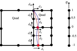
Figure 11.41 Enforcing compatibility of two different numbers of elements on a common edge using MPC.
• Substituting the values of η for the two additional nodes of the elements with shorter edges yields
![]() (11.18)
(11.18)
![]() (11.19)
(11.19)
which can be simplified to the following two constraint equations in the x direction:
![]() (11.20)
(11.20)
![]() (11.21)
(11.21)
Similarly, the constraint equations for the displacement in the y direction are obtained as
![]() (11.22)
(11.22)
![]() (11.23)
(11.23)
Equations (11.20) to (11.23) are a set of MPC equations for enforcing the compatibility of the interface between different numbers of elements.
11.10.3 Modeling of constraints by rigid body attachment
A rigid body attached to an elastic body will impose constraints on it. Figure 11.42 shows a rigid slab sitting on an elastic foundation. Assume that the rigid slab constrains only the vertical movement of the foundation, and it can move freely in the horizontal direction without affecting the foundation. To simulate such an effect of the rigid slab sitting on the foundation, MPC equations are required to enforce the four vertical DOFs on the foundation to follow the two DOFs on the slab.
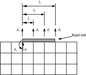
First, the four equations are:
 (11.24)
where q1 and q2 are, respectively, the translation and the rotation of the rigid slab. Then, eliminating the DOFs of the rigid body q1 and q2 from the above four equations leads to two MPC equations:
![]() (11.25)
(11.25)
![]() (11.26)
(11.26)
In the above example, the DOF in the x direction was not considered because it is assumed that the slab can move freely in the horizontal direction, and hence it will not provide any constraint to the foundation. If the rigid slab is perfectly connected to the foundation, the constraints on the DOFs in the x direction must also be considered.
11.11 Implementation of MPC equations
The previous sections have introduced some procedures for the derivation of MPC equations and some of its applications. However, how are such MPC equations implemented in the process of solving the global FEM system equation? Standard boundary conditions in the form of SPC equations can be easily implemented as each equation concerns only a single DOF. Many examples of implementing such standard boundary conditions of SPC equations can be found in examples and case studies in previous chapters. However, implementation of MPC equations usually requires more complex treatments to the global system equations.
Recall that the global system equation for a static system with DOF of n can be written in the following matrix form.
![]() (11.27)
(11.27)
where K is the stiffness matrix of n × n, D is the displacement vector of n × 1, and F is the external force vector of n × 1. If the system is constrained by m MPC equations, these equations can always be written in the following general matrix form:
![]() (11.28)
(11.28)
where C is a constant matrix of m × n (m < n), and Q is a constant matrix of m × 1. For example, let’s assume that there is a system of 10 DOFs (n = 10), we can then write the displacement vector as
![]() (11.29)
(11.29)
If the two (m = 2) MPC equations for this system are given as
![]() (11.30)
(11.30)
![]() (11.31)
(11.31)
which has the same form as that given by Eqs. (11.15) and (11.16). We then rewrite these MPCs in the following form of
![]() (11.32)
(11.32)
![]() (11.33)
(11.33)
From the above two equations, the matrix C is thus obtained as
 (11.34)
and the vector Q is a null vector given by
 (11.35)
The problem at hand is to obtain a solution for Eq. (11.27) subjected to the constraint equations given by Eq. (11.28). The following are two commonly used methods to obtain such a solution.
11.11.1 Lagrange multiplier method
First, the following m additional variables called Lagrange multipliers are introduced in this method as
![]() (11.36)
(11.36)
corresponding to m MPC equations. Each equation in the matrix equation of Eq. (11.28) is then multiplied by the corresponding λi, which yields
![]() (11.37)
(11.37)
The left-hand side of this equation is then added to the usual functional (refer to Eq. (3.2) of Chapter 3) to obtain the modified functional for the constraint system.
![]() (11.38)
(11.38)
The solution for the constraint system is found at the stationary point of the modified functional. The stationary condition requires the derivatives of Πp with respect to the Di and λi to vanish, and together with Eq. (11.37), gives
 (11.39)
which is the set of algebraic equations for the constraint system. Equation (11.39) is then solved instead of Eq. (11.27) to obtain the solution that satisfies the MPC equations. Note that from Eq. (11.39), KD + CTλ = F is a matrix equation consisting of n equations with n + m unknowns. CD = Q therefore provides the additional m equations that allow us to solve for all the unknowns including the m Lagrange multipliers.
The advantage of this method is that the constraint equations are satisfied exactly. However, it can be seen that the total number of unknowns is increased. In addition, the expanded stiffness matrix in Eq. (11.39) is non-positive definitely due to the presence of zero diagonal terms. Therefore, the efficiency of solving the system equations (11.39) is much lower than that of simply solving Eq. (11.27).
11.11.2 Penalty method
For the penalty method, Eq. (11.28) is re-written as
![]() (11.40)
(11.40)
so that t = 0 implies that the constraints are fully satisfied. The functional (refer to Eq. (3.2) of Chapter 3) can then be modified as
![]() (11.41)
(11.41)
where α is a diagonal matrix of “penalty numbers” (α1, α2, …, αm) that are constants chosen by the analyst. The stationary condition of the modified functional requires the derivatives of Πp with respect to the Di to vanish, which yields
![]() (11.42)
(11.42)
where CTαC is called a “penalty matrix.” From Eq. (11.42), it is seen that if α = 0, the constraints are ignored and the system equation reduces to the unconstrained equation Eq. (11.27). As αi becomes large, the penalty of violating the constraints becomes large. The terms with α in Eq. (11.42) overwhelm other terms. Therefore the solution satisfying Eq. (11.42) satisfies the constraints almost completely.
Note that the choice of αi can be a tricky task, as it depends on many factors in the FEM model. Considering that the discretization errors can be of comparable magnitude to those of not satisfying the constraint, it has been suggested that (Zienkiewicz and Taylor, 2000)
![]() (11.43)
(11.43)
where h is the characteristic size of the elements, and p denotes the order of the element used. The following simple method for calculating the penalty factor works well for most problems:
![]() (11.44)
(11.44)
It is also common to use
![]() (11.45)
(11.45)
Note that several trials may be required to decide on an appropriate penalty factor.
The advantage of this method is that the total number of unknowns is not changed and the system equations generally behave well. Therefore, the efficiency of solving the system equations Eq. (11.42) is almost the same as that of solving Eq. (11.27). However, the constraint equations can only be satisfied approximately, and the right choice of α can be ambiguous in some cases.
11.12 Review questions
1. What are the conditions of the use of mirror symmetry for reducing the size of the finite element discretization of a problem? Give your answer with reference to geometry, material, boundary conditions, and loading.
2. Indicate how the symmetric and anti-symmetric conditions can be used on a half-model to obtain the natural frequencies of a clamped-clamped beam of length L.
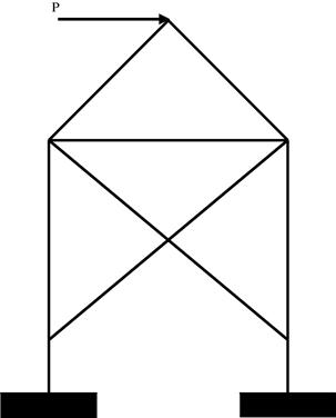
3. Figure 11.43 shows a frame structure subjected to a horizontal force at the top. Explain the use of symmetry to solve the problem with the aid of diagrams.
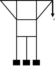
4. A symmetrical frame structure is under an asymmetric load P as shown in Figure 11.44. Describe with the aid of diagrams how you would use the symmetry to your advantage in modeling. Discuss the merits of using a symmetrical model in terms of the modeling and computational effort.
5. Explain why a transition element or MPCs are needed between the quadratic and linear elements shown in Figure 11.45.
6. Construct the shape functions in natural coordinates for the transition element shown in Figure 11.46. What is another way of solving the problem in Figure 11.45 if a transition element is not used?
7. Figure 11.47 shows a uniform mesh for a plane strain problem. The shaded block is rigid. Derive the MPC equations for nodes 1, 2, 3, and 4.

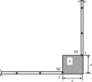
8. Figure 11.48 shows two planar beams perfectly joined to a rigid square block A (shaded) at right angles. The two beams are modeled using beam elements.
a. Derive the MPC equations for nodes 1 and 2.
b. Give an alternative method to model the rigid block, and comment on this method compared with the method using the MPC equations.
9. Consider a 2D plane strain problem, as shown in Figure 11.49, where a long beam is an extension of a main structure. The structure is subjected to dynamic loading.
a. The global response of the whole structural system is of interest. Design a mesh for the area within the large circle. If MPCs are needed, give the MPC equations.
b. The detailed results for the area within the small circle are of interest. Design a mesh for the area within the small circle. If MPCs are needed, give the MPC equations.

10. Figure 11.50 shows a rigid square body A (shaded) connected perfectly by two planar cantilever beams. You are requested to model this problem using a commercial FE package. The two beams should be modeled using beam elements.
a. Briefly explain three possible methods to model this problem, and the advantages and disadvantages of the methods.
b. Derive these MPC equations that can be used to model the rigid body A.

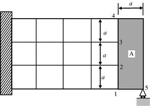
11. Figure 11.51 shows a rigid square body A (shaded) connected perfectly to a rectangular 2D solid. You are requested to model this problem using a commercial FE package using 2D solid elements. Derive MPC equations that can be used to properly model the rigid body A.
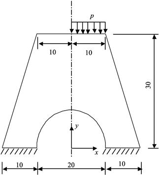
12. Figure 11.52 shows a bridge pier made of uniform material subjected to a uniformly distributed pressure on the right half of its top surface. The bridge pier can be idealized as a linear elastic 2D plane strain problem (in the x-y plane).
a. Explain your strategy to model this particular problem.
b. Sketch a mesh for this problem domain of your model using about 10 elements.
c. Provide all the boundary conditions, at relevant nodes, which are needed to solve this problem using your model.
d. How should the pressure be modeled?
13. How are the constraint equations implemented using the penalty method in the system equation KD = F? Here, K is the stiffness matrix for the global system, D is the displacement vector at all the nodes, and F is the external force vector acting at all the nodes. Assume that the constraint equations are given in the general form CD = Q, where C and Q are given constant matrices.
References
1. Liu GR. Meshfree Methods: Moving Beyond the Finite Element Method. second ed. Boca Raton: CRC Press; 2009.
2. Liu GR, Han X. Computational Inverse Techniques in Nondestructive Evaluation. CRC Press 2003.
3. Liu GR, Xi ZC. Elastic Waves in Anisotropic Laminates. CRC Press 2001.
4. Liu GR, Zhang GY. Smoothed Point Interpolation Methods—G Space Theory and Weakened Weak Forms. New York: World Scientific; 2013.
5. NAFEMS. A Finite Element Primer. Glasgow, UK: Department of Trade and Industry, National Engineering. Laboratory; 1986.
6. Zienkiewicz OC, Taylor RL. The Finite Element Method. fifth ed. Butterworth-Heinemann 2000.