Continuous-Time Signals and Systems1
José A. Apolinário Jr. and Carla L. Pagliari, Military Institute of Engineering (IME), Department of Electrical Engineering (SE/3), Rio de Janeiro, RJ, Brazil, [email protected], [email protected]
Abstract
This chapter provides a local source of information about analog signals and systems. The motivation for this chapter comes from the importance of having basic continuous-time theory prior or concomitant to the study of discrete-time systems. The scope of this chapter comprises the introduction of the basic concepts of signals, systems, and transforms in the continuous-time domain. We start by defining continuous-time signal, systems, and their properties. We focus on linear time-invariant systems, our main topic of interest and of great practical importance. We then move forward addressing the many ways to represent a linear system, always trying to analyze its input-output relationships. Finally, we discuss tools to be used in systems analysis; these tools, all having discrete-time counterparts, are transforms that unveil signals and systems behaviors in a transformed domain. We have prepared this material aiming an easy experience for a non-expert reader; nevertheless, for having a condensed amount of information gathered on a few pages, it might also be useful for experienced engineers. We tried to make a self contained text where beginners may refresh the fundamentals of continuous-time signal and systems without having to resort to other sources. The text is supported by examples, including figures and animations (videos), as well as a set of Matlab© codes, illustrating the concepts given throughout this chapter. We hope that the basic theory described herein proves useful for the development of the rest of this book.
Nomenclature
f frequency, in cycles per second or Hertz (Hz)
![]() input signal of a given continuous-time system, expressed in volt (V) when it corresponds to an input voltage;
input signal of a given continuous-time system, expressed in volt (V) when it corresponds to an input voltage; ![]() is usually used as the output signal
is usually used as the output signal
![]() angular frequency, in radian per second (rad/s) (it is sometimes referred to as frequency although corresponding to
angular frequency, in radian per second (rad/s) (it is sometimes referred to as frequency although corresponding to ![]() )
)
1.02.1 Introduction
Most signals present in our daily life are continuous in time such as music and speech. A signal is a function of an independent variable, usually an observation measured from the real world such as position, depth, temperature, pressure, or time. Continuous-time signals have a continuous independent variable. The velocity of a car could be considered a continuous-time signal if, at any time t, the velocity ![]() could be defined. A continuous-time signal with a continuous amplitude is usually called an analog signal, speech signal being a typical example.
could be defined. A continuous-time signal with a continuous amplitude is usually called an analog signal, speech signal being a typical example.
Signals convey information and are generated by electronic or natural means as when someone talks or plays a musical instrument. The goal of signal processing is to extract the useful information embedded in a signal.
Electronics for audio and last generation mobile phones must rely on universal concepts associated with the flow of information to make these devices fully functional. Therefore, a system designer, in order to have the necessary understanding of advanced topics, needs to master basic signals and systems theory. System theory could then be defined as the relation between signals, input and output signals.
As characterizing the complete input/output properties of a system through measurement is, in general, impossible, the idea is to infer the system response to non-measured inputs based on a limited number os measurements. System design is a chalenging task. However, several systems can be accurately modeled as linear systems. Hence, the designer has to create between the input and the output, an expected, or predictable, relationship that is always the same (time-invariant). In addition, for a range of possible input types, the system should generate a predictable output in accordance to the input/output relationship.
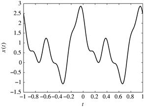
A continuous-time signal is defined on the continuum of time values as the one depicted in Figure 2.1, ![]() for
for ![]() .
.
Although signals are real mathematical functions, some transformations can produce complex signals that have both real and imaginary parts. Therefore, throughout this book, complex domain equivalents of real signals will certainly appear.
Elementary continuous-time signals are the basis to build more intricate signals. The unit step signal, ![]() , displayed by Figure 2.2a is equal to 1 for all time greater than or equal to zero, and is equal to zero for all time less than zero. A step of height K can be made with
, displayed by Figure 2.2a is equal to 1 for all time greater than or equal to zero, and is equal to zero for all time less than zero. A step of height K can be made with ![]() .
.

Figure 2.2 Basic continuous-time signals: (a) unit-step signal ![]() , (b) unit-area pulse, (c) impulse signal (unit-area pulse when
, (b) unit-area pulse, (c) impulse signal (unit-area pulse when ![]() ), and (d) exponential signal.
), and (d) exponential signal.
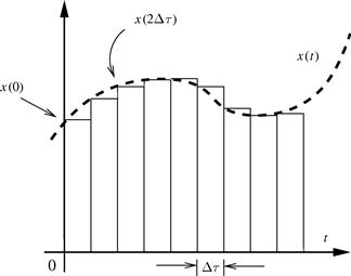
A unit area pulse is pictured in Figure 2.2b; as ![]() gets smaller, the pulse gets higher and narrower with a constant area of one (unit area). We can see the impulse signal, in Figure 2.2c, as a limiting case of the pulse signal when the pulse is infinitely narrow. The impulse response will help to estimate how the system will respond to other possible stimuli, and we will further explore this topic on the next section.
gets smaller, the pulse gets higher and narrower with a constant area of one (unit area). We can see the impulse signal, in Figure 2.2c, as a limiting case of the pulse signal when the pulse is infinitely narrow. The impulse response will help to estimate how the system will respond to other possible stimuli, and we will further explore this topic on the next section.
Exponential signals are important for signals and systems as eigensignals of linear time-invariant systems. In Figure 2.2d, for A and ![]() being real numbers,
being real numbers, ![]() negative, the signal is a decaying exponential. When
negative, the signal is a decaying exponential. When ![]() is a complex number, the signal is called a complex exponential signal. The periodic signals sine and cosine are used for modeling the interaction of signals and systems, and the usage of complex exponentials to manipulate sinusoidal functions turns trigonometry into elementary arithmetic and algebra.
is a complex number, the signal is called a complex exponential signal. The periodic signals sine and cosine are used for modeling the interaction of signals and systems, and the usage of complex exponentials to manipulate sinusoidal functions turns trigonometry into elementary arithmetic and algebra.
1.02.2 Continuous-time systems
We start this section by providing a simplified classification of continuous-time systems in order to focus on our main interest: a linear and time-invariant (LTI) system.
Why are linearity and time-invariance important? In general, real world systems can be successfully modeled by theoretical LTI systems; in an electrical circuit, for instance, a system can be designed using a well developed linear theory (valid for LTI systems) and be implemented using real components such as resistors, inductors, and capacitors. Even though the physical components, strictly speaking, do not comply with linearity and time-invariance for any input signals, the circuit will work quite well under reasonable conditions (input voltages constrained to the linear working ranges of the components).
A system can be modeled as a function that transforms, or maps, the input signal into a new output signal. Let a continuous-time system be represented as in Figure 2.3 where ![]() is the input signal and
is the input signal and ![]() , its output signal, corresponds to a transformation applied to the input signal:
, its output signal, corresponds to a transformation applied to the input signal: ![]() .
.

Figure 2.3 A generic continuous-time system representing the output signal as a transformation applied to the input signal: ![]() .
.
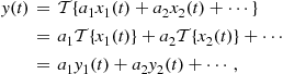
The two following properties define a LTI system.Linearity: A continuous-time system is said to be linear if a linear combination of input signals, when applied to this system, produces an output that corresponds to a linear combination of individual outputs, i.e.,
 (2.1)
(2.1)
where ![]() .Time-invariance: A continuous-time system is said to be time-invariant when the output signal,
.Time-invariance: A continuous-time system is said to be time-invariant when the output signal, ![]() , corresponding to an input signal
, corresponding to an input signal ![]() , will be a delayed version of the original output,
, will be a delayed version of the original output, ![]() , whenever the input is delayed accordingly, i.e.,
, whenever the input is delayed accordingly, i.e.,
![]()
The transformation caused in the input signal by a linear time-invariant system may be represented in a number of ways: with a set of differential equations, with the help of a set of state-variables, with the aid of the concept of the impulse response, or in a transformed domain.
Let the circuit in Figure 2.4 be an example of a continuous-time system where the input ![]() corresponds to the voltage between terminals
corresponds to the voltage between terminals ![]() and
and ![]() while its output
while its output ![]() is described by the voltage between terminals
is described by the voltage between terminals ![]() and
and ![]() .
.
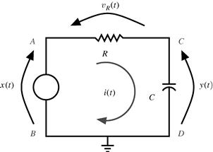
Figure 2.4 An example of an electric circuit representing a continuous-time system with input ![]() and output
and output ![]() .
.
We know for this circuit that ![]() and that the current in the capacitor,
and that the current in the capacitor, ![]() , corresponds to
, corresponds to ![]() . Therefore,
. Therefore, ![]() , and we can write
, and we can write
![]() (2.2)
(2.2)
which is an input-output (external) representation of a continuous-time system given as a differential equation.
Another representation of a linear system, widely used in control theory, is the state-space representation. This representation will be presented in the next section since it is better explored for systems having a higher order differential equation.
In order to find an explicit expression for ![]() as a function of
as a function of ![]() , we need to solve the differential equation. The complete solution of this system, as shall be seen in the following section, is given by the sum of an homogeneous solution (zero-input solution or natural response) and a particular solution (zero-state solution or forced solution):
, we need to solve the differential equation. The complete solution of this system, as shall be seen in the following section, is given by the sum of an homogeneous solution (zero-input solution or natural response) and a particular solution (zero-state solution or forced solution):
![]() (2.3)
(2.3)
The homogeneous solution, in our example, is obtained from (2.2) by setting ![]() . Since this solution and its derivatives must comply with the homogeneous differential equation, its usual choice is an exponential function such as
. Since this solution and its derivatives must comply with the homogeneous differential equation, its usual choice is an exponential function such as ![]() being, in general, a complex number. Replacing this general expression in the homogeneous differential equation, we obtain
being, in general, a complex number. Replacing this general expression in the homogeneous differential equation, we obtain ![]() (characteristic equation) and, therefore,
(characteristic equation) and, therefore, ![]() , such that the homogenous solution becomes
, such that the homogenous solution becomes
![]() (2.4)
(2.4)
where K is a constant.
The particular solution is usually of the same form as the forcing function (input voltage ![]() in our example) and it must comply with the differential equation without an arbitrary constant. In our example, if
in our example) and it must comply with the differential equation without an arbitrary constant. In our example, if ![]() would be
would be ![]() .
.
If we set ![]() , the step function which can be seen as a DC voltage of 1 Volt switched at time instant
, the step function which can be seen as a DC voltage of 1 Volt switched at time instant ![]() , the forced solution is assumed to be equal to one when
, the forced solution is assumed to be equal to one when ![]() . For this particular input
. For this particular input ![]() , the output signal is given by
, the output signal is given by ![]() . Constant K is obtained with the knowledge of the initial charge of the capacitor (initial conditions); assuming it is not charged (
. Constant K is obtained with the knowledge of the initial charge of the capacitor (initial conditions); assuming it is not charged (![]() ), we have
), we have
![]() (2.5)
(2.5)
which can be observed in Figure 2.5.

Figure 2.5 Input and output signals of the system depicted in Figure 2.4. See refgroup Refmmcvideo1Video 1 to watch animation.
Note that, for this case where ![]() , the output
, the output ![]() is known as the step response, i.e.,
is known as the step response, i.e., ![]() . Moreover, since the impulse
. Moreover, since the impulse ![]() corresponds to the derivative of
corresponds to the derivative of ![]() , and the system is LTI (linear and time-invariant), we may write that
, and the system is LTI (linear and time-invariant), we may write that ![]() which corresponds to
which corresponds to ![]() , the transformation applied to the impulse signal leading to
, the transformation applied to the impulse signal leading to
![]() (2.6)
(2.6)
![]() known as the impulse response or
known as the impulse response or ![]() .
.
The impulse response is, particularly, an important characterization of a linear system. It will help to estimate how the system will respond to other stimuli. In order to show the relevance of this, let us define the unit impulse as
![]() (2.7)
(2.7)
such that we may see an input signal ![]() as in Figure 2.6:
as in Figure 2.6:
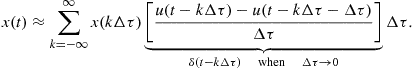 (2.8)
(2.8)
The idea is to show that any signal, e.g., ![]() , can be expressed as a sum of scaled and shifted impulse functions.
, can be expressed as a sum of scaled and shifted impulse functions.
In (2.8), making ![]() and representing the resulting continuous time by
and representing the resulting continuous time by ![]() instead of
instead of ![]() , we can use the integral instead of the summation and find
, we can use the integral instead of the summation and find
![]() (2.9)
(2.9)
In a LTI system, using the previous expression as an input signal to compute the output ![]() , we obtain
, we obtain ![]() such that the output signal can be written as
such that the output signal can be written as
![]() (2.10)
(2.10)
This expression is known as the convolution integral between the input signal and the system impulse response, and is represented as
![]() (2.11)
(2.11)
Please note that the output signal provided by the convolution integral corresponds to the zero-state solution.
From Figure 2.6, another approximation for ![]() can be devised, leading to another expression relating input and output signals. At a certain instant
can be devised, leading to another expression relating input and output signals. At a certain instant ![]() , let the angle of a tangent line to the curve of
, let the angle of a tangent line to the curve of ![]() be
be ![]() such that
such that ![]() . Assuming a very small
. Assuming a very small ![]() , this tangent can be approximated by
, this tangent can be approximated by ![]() such that
such that
![]() (2.12)
(2.12)
Knowing each increment at every instant ![]() , we can visualize an approximation for
, we can visualize an approximation for ![]() as a sum of shifted and weighted step functions
as a sum of shifted and weighted step functions ![]() , i.e.,
, i.e.,
![]() (2.13)
(2.13)
From the previous expression, if we once more, as in (2.9), make ![]() and represent the resulting continuous-time by
and represent the resulting continuous-time by ![]() instead of
instead of ![]() , we can drop the summation and use the integral to obtain
, we can drop the summation and use the integral to obtain
![]() (2.14)
(2.14)
Assuming, again, that the system is LTI, we use the last expression as an input signal to compute the output ![]() , obtaining
, obtaining ![]() which can be written as
which can be written as
![]() (2.15)
(2.15)
or, ![]() being the step-response, as
being the step-response, as
![]() (2.16)
(2.16)
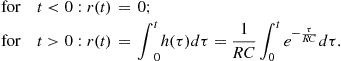
In our example from Figure 2.4, taking the derivative of ![]() , we obtain the impulse response (the computation of this derivative is somehow tricky for we must bear in mind that the voltage in the terminals of a capacitor cannot present discontinuities; just as in the case of the current through an inductor) as:
, we obtain the impulse response (the computation of this derivative is somehow tricky for we must bear in mind that the voltage in the terminals of a capacitor cannot present discontinuities; just as in the case of the current through an inductor) as:
![]() (2.17)
(2.17)
In order to have a graphical interpretation of the convolution, we make ![]() in (2.11) and use
in (2.11) and use
![]() (2.18)
(2.18)
we then compute this integral, as indicated in Figure 2.7, in two parts:
 (2.19)
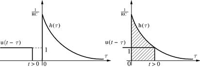
Figure 2.7 Graphical interpretation of the convolution integral. See refgroup Refmmcvideo2Video 2 to watch animation.
Finally, from (2.19), we obtain ![]() , as previously known.
, as previously known.
A few mathematical properties of the convolution are listed in the following:
The properties of convolution can be used to analyze different system combinations. For example, if two systems with impulse responses ![]() and
and ![]() are cascaded, the whole cascade system will present the impulse response
are cascaded, the whole cascade system will present the impulse response ![]() . The commutative property allows the order of the systems of the cascade combination to be changed without affecting the whole system’s response.
. The commutative property allows the order of the systems of the cascade combination to be changed without affecting the whole system’s response.
Two other important system properties are causability and stability.Causability: A causal system, also known as non-anticipative system, is a system in which its output ![]() depends only in the current and past (not future) information about
depends only in the current and past (not future) information about ![]() . A non-causal, or anticipative, system is actually not feasible to be implemented in real-life. For example,
. A non-causal, or anticipative, system is actually not feasible to be implemented in real-life. For example, ![]() is non-causal, whereas
is non-causal, whereas ![]() is causal.
is causal.
With respect to the impulse response, it is also worth mentioning that, for a causal system, ![]() for
for ![]() .Stability: A system is stable if and only if every bounded input produces a bounded output, i.e., if
.Stability: A system is stable if and only if every bounded input produces a bounded output, i.e., if ![]() then
then ![]() for all values of
for all values of ![]() .
.
More about stability will be addressed in a forthcoming section, after the concept of poles and zeros is introduced.
The classic texts for the subjects discussed in this section include [1–5].
1.02.3 Differential equations
In many engineering applications, the behavior of a system is described by a differential equation. A differential equation is merely an equation with derivative of at least one of its variables. Two simple examples follow:
![]() (2.20)
(2.20)
![]() (2.21)
(2.21)
where a, b, and c are constants.
In (2.20), we observe an ordinary differential equation, i.e., there is only one independent variable and ![]() being the independent variable. On the other hand, in (2.21), we have a partial differential equation where
being the independent variable. On the other hand, in (2.21), we have a partial differential equation where ![]() and y being two independent variables. Both examples have order 2 (highest derivative appearing in the equation) and degree 1 (power of the highest derivative term).
and y being two independent variables. Both examples have order 2 (highest derivative appearing in the equation) and degree 1 (power of the highest derivative term).
This section deals with the solution of differential equations usually employed to represent the mathematical relationship between input and output signals of a linear system. We are therefore most interested in linear differential equations with constant coefficients having the following general form:
![]() (2.22)
(2.22)
The expression on the right side of (2.22) is known as forcing function, ![]() . When
. When ![]() , the differential equation is known as homogeneous while a non-zero forcing function corresponds to a nonhomogeneous differential equation such as in
, the differential equation is known as homogeneous while a non-zero forcing function corresponds to a nonhomogeneous differential equation such as in
![]() (2.23)
(2.23)
As mentioned in the previous section, the general solution of a differential equation as the one in (2.22) is given by the sum of two expressions: ![]() , the solution of the associated homogeneous differential equation
, the solution of the associated homogeneous differential equation
![]() (2.24)
(2.24)
and a particular solution of the nonhomogeneous equation, ![]() , such that
, such that
![]() (2.25)
(2.25)
Solution of the homogeneous equation: The natural response of a linear system is given by ![]() , the solution of (2.24). Due to the fact that a linear combination of
, the solution of (2.24). Due to the fact that a linear combination of ![]() and its derivatives must be equal to zero in order to comply with (2.24), it may be postulated that it has the form
and its derivatives must be equal to zero in order to comply with (2.24), it may be postulated that it has the form
![]() (2.26)
(2.26)
where s is a constant to be determined.
Replacing the assumed solution in (2.24), we obtain, after simplification, the characteristic (or auxiliary equation)
![]() (2.27)
(2.27)
Assuming N distinct roots of the polynomial in (2.27), ![]() to
to ![]() , the homogeneous solution is obtained as a linear combination of N exponentials as in
, the homogeneous solution is obtained as a linear combination of N exponentials as in
![]() (2.28)
(2.28)
Two special cases follow.
1. Non-distinct roots: if, for instance, ![]() , it is possible to show that
, it is possible to show that ![]() and
and ![]() are independent solutions leading to
are independent solutions leading to
![]()
2. Characteristic equation with complex roots: it is known that, for real coefficients (![]() to
to ![]() ), all complex roots will occur in complex conjugate pairs such as
), all complex roots will occur in complex conjugate pairs such as ![]() and
and ![]() ,
, ![]() and
and ![]() being real numbers. Hence, the solution would be
being real numbers. Hence, the solution would be
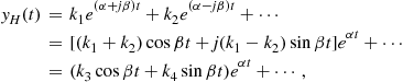
![]() and
and ![]() being real numbers if we make
being real numbers if we make ![]() . In that case, we will have
. In that case, we will have
![]()
with ![]() and
and ![]() . Also note from the last expression that, in order to have a stable system (bounded output),
. Also note from the last expression that, in order to have a stable system (bounded output), ![]() should be negative (causing a decaying exponential).
should be negative (causing a decaying exponential).
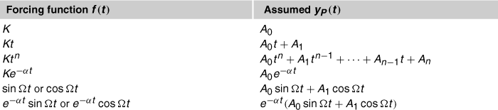
Solution of the nonhomogeneous equation: A (any) forced solution of the nonhomogeneous equation must satisfy (2.23) containing no arbitrary constant. A usual way to find the forced solution is employing the so called method of undetermined coefficients: it consists in estimating a general form for ![]() from
from ![]() , the forcing function. The coefficients (
, the forcing function. The coefficients (![]() ), as seen in Table 2.1 that shows the most common assumed solutions for each forced function, are to be determined in order to comply with the nonhomogeneous equation. A special case is treated slightly differently: when a term of
), as seen in Table 2.1 that shows the most common assumed solutions for each forced function, are to be determined in order to comply with the nonhomogeneous equation. A special case is treated slightly differently: when a term of ![]() corresponds to a term of
corresponds to a term of ![]() , the corresponding term in
, the corresponding term in ![]() must be multiplied by t. Also, when we find non-distinct roots of the characteristic equation (assume multiplicity m as an example), the corresponding term in
must be multiplied by t. Also, when we find non-distinct roots of the characteristic equation (assume multiplicity m as an example), the corresponding term in ![]() shall be multiplied by
shall be multiplied by ![]() .
.
An example of a second order ordinary differential equation (ODE) with constant coefficients is considered as follows:
![]() (2.29)
(2.29)
where ![]() (in
(in ![]() ),
), ![]() (in H),
(in H), ![]() (in F), and
(in F), and ![]() (in V).
(in V).
This equation describes the input ![]() output relationship of the electrical circuit shown in Figure 2.8 for
output relationship of the electrical circuit shown in Figure 2.8 for ![]() .
.
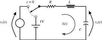
Figure 2.8 RLC series circuit with a voltage source as input and the voltage in the capacitor as output.
Replacing the values of the components and the input voltage, the ODE becomes
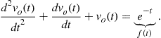 (2.30)
The associated characteristic equation ![]() has roots
has roots ![]() leading to an homogeneous solution given by
leading to an homogeneous solution given by
 (2.31)
Next, from the forcing function ![]() , we assume
, we assume ![]() and replace it in (2.30), resulting in
and replace it in (2.30), resulting in ![]() such that:
such that:
 (2.32)
where ![]() and
and ![]() (or
(or ![]() and
and ![]() ) are constants to be obtained from previous knowledge of the physical system, the RLC circuit in this example. This knowledge comes as the initial conditions: an N-order differential equation having N constants and requiring N initial conditions.Initial conditions: Usually, the differential equation describing the behavior of an electrical circuit is valid for any time
) are constants to be obtained from previous knowledge of the physical system, the RLC circuit in this example. This knowledge comes as the initial conditions: an N-order differential equation having N constants and requiring N initial conditions.Initial conditions: Usually, the differential equation describing the behavior of an electrical circuit is valid for any time ![]() (instant 0 assumed the initial reference in time); the initial conditions corresponds to the solution (and its
(instant 0 assumed the initial reference in time); the initial conditions corresponds to the solution (and its ![]() derivatives) at
derivatives) at ![]() . In the absence of pulses, the voltage at the terminals of a capacitance and the current through an inductance cannot vary instantaneously and must be the same value at
. In the absence of pulses, the voltage at the terminals of a capacitance and the current through an inductance cannot vary instantaneously and must be the same value at ![]() and
and ![]() .
.
In the case of our example, based on the fact that there is a key switching ![]() to the RLC series at
to the RLC series at ![]() , we can say that the voltage across the inductor is
, we can say that the voltage across the inductor is ![]() (the capacitor assumed charged with the DC voltage). Therefore, since the voltage across C and the current through L do not alter instantaneously, we know that
(the capacitor assumed charged with the DC voltage). Therefore, since the voltage across C and the current through L do not alter instantaneously, we know that ![]() and
and ![]() . Since we know that
. Since we know that ![]() , we have
, we have ![]() . With these initial conditions and from (2.32), we find
. With these initial conditions and from (2.32), we find ![]() and
and ![]() .
.
Finally, the general solution is given as
![]() (2.33)
(2.33)
Figure 2.9 shows ![]() for
for ![]() . An easy way to obtain this result with Matlab© is:
. An easy way to obtain this result with Matlab© is:
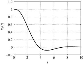
Figure 2.9 Output voltage as a function of time, ![]() , for the circuit in Figure 2.8. See refgroup Refmmcvideo3Video 3 to watch animation.
, for the circuit in Figure 2.8. See refgroup Refmmcvideo3Video 3 to watch animation.
To end this section, we represent this example using the state-space approach. We first rewrite (2.29) using the first and the second derivatives of ![]() as
as ![]() and
and ![]() , respectively, and also
, respectively, and also ![]() as in
as in
![]() (2.34)
(2.34)
In this representation, we define a state vector ![]() and its derivative
and its derivative ![]() , and from these definitions we write the state equation and the output equation:
, and from these definitions we write the state equation and the output equation:
 (2.35)
where ![]() is known as the state matrix,
is known as the state matrix, ![]() as the input matrix,
as the input matrix, ![]() as the output matrix, and D (equal to zero in this example) would be the feedthrough (or feedforward) matrix.
as the output matrix, and D (equal to zero in this example) would be the feedthrough (or feedforward) matrix.
1.02.4 Laplace transform: definition and properties
The Laplace transform [10] is named after the French mathematician Pierre-Simon Laplace. It is an important tool for solving differential equations, and it is very useful for designing and analyzing linear systems [11].
The Laplace transform is a mathematical operation that maps, or transforms, a variable (or function) from its original domain into the Laplace domain, or s domain. This transform produces a time-domain response to transitioning inputs, whenever time-domain behavior is more interesting than frequency-domain behavior. When solving engineering problems one has to model a physical phenomenon that is dependent on the rates of change of a function (e.g., the velocity of a car as mentioned in Section 1.02.1). Hence, calculus associated with differential equations (Section 1.02.3), that model the phenomenon, are the natural candidates to be the mathematical tools. However, calculus solves (ordinary) differential equations provided the functions are continuous and with continuous derivatives. In addition, engineering problems have often to deal with impulsive, non-periodic or piecewise-defined input signals.
The Fourier transform, to be addressed in Section 1.02.7, is also an important tool for signal analysis, as well as for linear filter design. However, while the unit-step function (Figure 2.2a), discontinuous at time ![]() , has a Laplace transform, its forward Fourier integral does not converge. The Laplace transform is particularly useful for input terms that are impulsive, non-periodic or piecewise-defined [4].
, has a Laplace transform, its forward Fourier integral does not converge. The Laplace transform is particularly useful for input terms that are impulsive, non-periodic or piecewise-defined [4].
The Laplace transform maps the time-domain into the s-domain, with ![]() , converting integral and differential equations into algebraic equations. The function is mapped (transformed) to the s-domain, eliminating all the derivatives. Hence, solving the equation becomes simple algebra in the s-domain and the result is transformed back to the time-domain. The Laplace transform converts a time-domain 1-D signal,
, converting integral and differential equations into algebraic equations. The function is mapped (transformed) to the s-domain, eliminating all the derivatives. Hence, solving the equation becomes simple algebra in the s-domain and the result is transformed back to the time-domain. The Laplace transform converts a time-domain 1-D signal, ![]() , into a complex representation,
, into a complex representation, ![]() , defined over a complex plane (s-plane). The complex plane is spanned by the variables
, defined over a complex plane (s-plane). The complex plane is spanned by the variables ![]() (real axis) and
(real axis) and ![]() (imaginary axis) [5].
(imaginary axis) [5].
The two-sided (or bilateral) Laplace transform of a signal ![]() is the function
is the function ![]() defined by:
defined by:
![]() (2.36)
(2.36)
The notation ![]() denotes that
denotes that ![]() is the Laplace transform of
is the Laplace transform of ![]() . Conversely, the notation
. Conversely, the notation ![]() denotes that
denotes that ![]() is the inverse Laplace transform of
is the inverse Laplace transform of ![]() . This relationship is expressed with the notation
. This relationship is expressed with the notation ![]() .
.
As ![]() , Eq. (2.36) can be rewritten as
, Eq. (2.36) can be rewritten as
![]() (2.37)
(2.37)
This way, one can identify that the Laplace transform real part (![]() ) represents the contribution of the (combined) exponential and cosine terms to
) represents the contribution of the (combined) exponential and cosine terms to ![]() , while its imaginary part (
, while its imaginary part (![]() ) represents the contribution of the (combined) exponential and sine terms to
) represents the contribution of the (combined) exponential and sine terms to ![]() . As the term
. As the term ![]() is an eigenfunction, we can state that the Laplace transform represents time-domain signals in the s-domain as weighted combinations of eigensignals.
is an eigenfunction, we can state that the Laplace transform represents time-domain signals in the s-domain as weighted combinations of eigensignals.
For those signals equal to zero for ![]() , the limits on the integral are changed for the one-sided (or unilateral) Laplace transform:
, the limits on the integral are changed for the one-sided (or unilateral) Laplace transform:
with ![]() for
for ![]() , in order to deal with signals that present singularities at the origin, i.e., at
, in order to deal with signals that present singularities at the origin, i.e., at ![]() .
.
As the interest will be in signals defined for ![]() , let us find the one-sided Laplace transform of
, let us find the one-sided Laplace transform of ![]() :
:
![]() (2.39)
(2.39)
The integral, in (2.39), defining ![]() is true if
is true if ![]() as
as ![]()
![]() with
with ![]() , which is the region of convergence of
, which is the region of convergence of ![]() .
.
As the analysis of convergence, as well as the conditions that guarantee the existence of the Laplace integral are beyond the scope of this chapter, please refer to [4,5].
For a given ![]() , the integral may converge for some values of
, the integral may converge for some values of ![]() , but not for others. So, we have to guarantee the existence of the integral, i.e.,
, but not for others. So, we have to guarantee the existence of the integral, i.e., ![]() has to be absolutely integrable. The region of convergence (ROC) of the integral in the complex s-plane should be specified for each transform
has to be absolutely integrable. The region of convergence (ROC) of the integral in the complex s-plane should be specified for each transform ![]() , that exists if and only if the argument s is inside the ROC. The transformed signal,
, that exists if and only if the argument s is inside the ROC. The transformed signal, ![]() will be well defined for a range of values in the s-domain that is the ROC, which is always given in association with the transform itself.
will be well defined for a range of values in the s-domain that is the ROC, which is always given in association with the transform itself.
When ![]() , so that
, so that ![]() , the Laplace transform reverts to the Fourier transform, i.e.,
, the Laplace transform reverts to the Fourier transform, i.e., ![]() has a Fourier transform if the ROC of the Laplace transform in the s-plane includes the imaginary axis.
has a Fourier transform if the ROC of the Laplace transform in the s-plane includes the imaginary axis.
For finite duration signals that are absolutely integrable, the ROC contains the entire s-plane. As ![]() cannot uniquely define
cannot uniquely define ![]() , it is necessary
, it is necessary ![]() and the ROC. If we wish to find the Laplace transform of a one-sided real exponential function
and the ROC. If we wish to find the Laplace transform of a one-sided real exponential function ![]() , given by:
, given by:
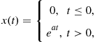 (2.40)
we have
![]() (2.41)
(2.41)
The integral of (2.41) converges if ![]() , and the ROC is the region of the s-plane to the right of
, and the ROC is the region of the s-plane to the right of ![]() , as pictured in Figure 2.10. If
, as pictured in Figure 2.10. If ![]() the integral does not converge as
the integral does not converge as ![]() , and if
, and if ![]() we cannot determine
we cannot determine ![]() .
.
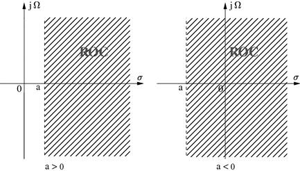
Figure 2.10 Region of Convergence (ROC) on the s-plane for the signal defined by Eq. (2.40). Note that, for a stable signal (![]() ), the ROC contains the vertical axis
), the ROC contains the vertical axis ![]() .
.
In other words, if a signal ![]() is nonzero only for
is nonzero only for ![]() , the ROC of its Laplace transform lies to the right hand side of its poles (please refer to Section 1.02.5). Additionally, the ROC does not contain any pole. Poles are points where the Laplace transform reaches infinite value in the s-plane (e.g.,
, the ROC of its Laplace transform lies to the right hand side of its poles (please refer to Section 1.02.5). Additionally, the ROC does not contain any pole. Poles are points where the Laplace transform reaches infinite value in the s-plane (e.g., ![]() in Figure 2.10).
in Figure 2.10).
An example of the two-sided Laplace transform of a right-sided exponential function ![]() , is given by
, is given by
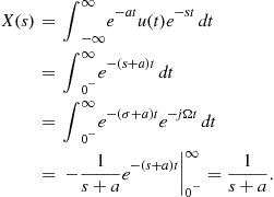 (2.42)
As the term ![]() is sinusoidal, only
is sinusoidal, only ![]() is important, i.e., the integral given by (2.42), when t tends to infinity, converges if
is important, i.e., the integral given by (2.42), when t tends to infinity, converges if ![]() is finite (
is finite (![]() ) in order to the exponential function to decay. The integral of Eq. (2.42) converges if
) in order to the exponential function to decay. The integral of Eq. (2.42) converges if ![]() , i.e., if
, i.e., if ![]() , and the ROC is the region of the s-plane to the right of
, and the ROC is the region of the s-plane to the right of ![]() , as pictured in the left side of Figure 2.11. The ROC of the Laplace transform of a right-sided signal is to the right of its rightmost pole.
, as pictured in the left side of Figure 2.11. The ROC of the Laplace transform of a right-sided signal is to the right of its rightmost pole.

Figure 2.11 Regions of Convergence (ROCs) on the s-plane: (a) for right-sided signals, ![]() , and (b) for left-sided signals,
, and (b) for left-sided signals, ![]() .
.
If, we wish to find the two-sided Laplace transform of a left-sided signal, ![]() , we have
, we have
 (2.43)
The integral of Eq. (2.43) converges if ![]() , and the ROC is the region of the s-plane to the left of
, and the ROC is the region of the s-plane to the left of ![]() , as pictured in the right side of Figure 2.11. The ROC of the Laplace transform of a left-sided signal is to the left of its leftmost pole.
, as pictured in the right side of Figure 2.11. The ROC of the Laplace transform of a left-sided signal is to the left of its leftmost pole.
For for causal systems, where ![]() , and right-sided signals, where
, and right-sided signals, where ![]() , the unilateral (one-sided) and bilateral (two-sided) transforms are equal. However, it is important to stress that some properties change, such as the differentiation property reduced to
, the unilateral (one-sided) and bilateral (two-sided) transforms are equal. However, it is important to stress that some properties change, such as the differentiation property reduced to ![]() for the bilateral case. Conversely, other properties, such as convolution, hold as is, provided the system is causal and the input starts at
for the bilateral case. Conversely, other properties, such as convolution, hold as is, provided the system is causal and the input starts at ![]() .
.
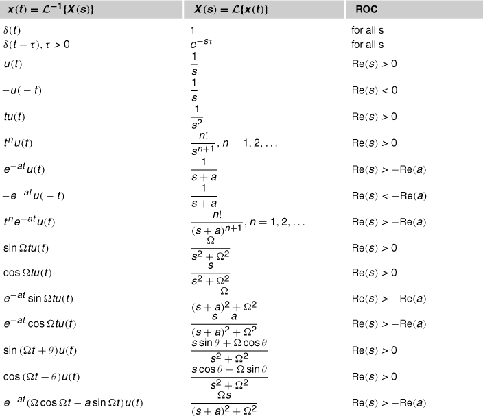
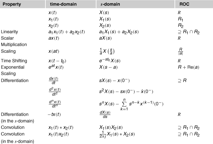
Common Laplace transform pairs [12] are summarized in Table 2.2.
Recalling Figure 2.3 from Section 1.02.1, where ![]() is the input to a linear system with impulse response
is the input to a linear system with impulse response ![]() , to obtain the output
, to obtain the output ![]() one could convolve
one could convolve ![]() with
with ![]() (2.11). However, if
(2.11). However, if ![]() and
and ![]() are the associated Laplace transforms, the (computationally demanding) operation of convolution in the time-domain is mapped into a (simple) operation of multiplication in the s-domain):
are the associated Laplace transforms, the (computationally demanding) operation of convolution in the time-domain is mapped into a (simple) operation of multiplication in the s-domain):
![]() (2.44)
(2.44)
Equation (2.44) shows that convolution in time-domain is equivalent to multiplication in Laplace domain. In the following, some properties of the Laplace transform disclose the symmetry between operations in the time- and s-domains.Linearity: If ![]() , ROC = R1, and
, ROC = R1, and ![]() , ROC = R2, then
, ROC = R2, then
![]() (2.45)
(2.45)
with ![]() and
and ![]() being constants and ROC
being constants and ROC ![]() . The Laplace transform is a linear operation.Time shifting: If
. The Laplace transform is a linear operation.Time shifting: If ![]() , ROC = R, then
, ROC = R, then ![]() , ROC = R.
, ROC = R.
 (2.46)
where ![]() . Time shifting (or time delay) in the time-domain is equivalent to modulation (alteration of the magnitude and phase) in the s-domain.Exponential scaling (frequency shifting): If
. Time shifting (or time delay) in the time-domain is equivalent to modulation (alteration of the magnitude and phase) in the s-domain.Exponential scaling (frequency shifting): If ![]() , ROC = R, then
, ROC = R, then ![]() .
.
![]() (2.47)
(2.47)
Modulation in the time-domain is equivalent to shifting in the s-domain.Convolution: If ![]() , ROC =
, ROC = ![]() , and
, and ![]() , ROC =
, ROC = ![]() , then
, then ![]() , ROC
, ROC ![]() :
:
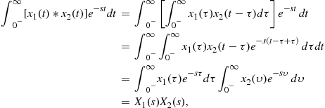 (2.48)
where in the inner integral ![]() . Convolution in time-domain is equivalent to multiplication in the s-domain.Differentiation in time: If
. Convolution in time-domain is equivalent to multiplication in the s-domain.Differentiation in time: If ![]() , ROC = R, then
, ROC = R, then ![]() , ROC
, ROC ![]() . Integrating by parts, we have:
. Integrating by parts, we have:
 (2.49)
where any jump from ![]() to
to ![]() is considered. In other words, the Laplace transform of a derivative of a function is a combination of the transform of the function, multiplicated by s, and its initial value. This property is quite useful as a differential equation in time can be turned into an algebraic equation in the Laplace domain, where it can be solved and mapped back into the time-domain (Inverse Laplace Transform).
is considered. In other words, the Laplace transform of a derivative of a function is a combination of the transform of the function, multiplicated by s, and its initial value. This property is quite useful as a differential equation in time can be turned into an algebraic equation in the Laplace domain, where it can be solved and mapped back into the time-domain (Inverse Laplace Transform).
The initial- and final-value theorems show that, the initial and the final values of a signal in the time-domain can be obtained from its Laplace transform without knowing its expression in the time-domain.Initial-value theorem: Considering stable the LTI system, that generated the signal ![]() , then
, then
![]() (2.50)
(2.50)
From the differentiation in time property, we have that ![]() . By taking the limit when
. By taking the limit when ![]() of the first expression of (2.49), we find
of the first expression of (2.49), we find
 (2.51)
If we take the limit of s to ![]() in the result of (2.49), we have
in the result of (2.49), we have
![]() (2.52)
(2.52)
then we can equal the results of (2.52) and (2.51) and get
![]() (2.53)
(2.53)
As the right-hand side of (2.53) is obtained taking the limit when ![]() of the result of (2.49), we can see from (2.51) and (2.53) that
of the result of (2.49), we can see from (2.51) and (2.53) that
![]() (2.54)
(2.54)
The initial-value theorem provides the behavior of a signal in the time-domain for small time intervals, i.e., for ![]() . In other words, it determines the initial values of a function in time from its expression in the s-domain, which is particularly useful in circuits and systems.Final-value theorem: Considering that the LTI system that generated the signal
. In other words, it determines the initial values of a function in time from its expression in the s-domain, which is particularly useful in circuits and systems.Final-value theorem: Considering that the LTI system that generated the signal ![]() is stable, then
is stable, then
![]() (2.55)
(2.55)
From the differentiation in time property, we have that ![]() . By taking the limit when
. By taking the limit when ![]() of the first expression of (2.49), we have
of the first expression of (2.49), we have
![]() (2.56)
(2.56)
![]()
If we take the limit when ![]() of the last expression of (2.49), we get
of the last expression of (2.49), we get
![]() (2.57)
(2.57)
then, we can write
![]() (2.58)
(2.58)
As the right-hand side of (2.58) is obtained taking the limit when ![]() of the result of (2.49), we can see from (2.56) and (2.58) that
of the result of (2.49), we can see from (2.56) and (2.58) that
![]() (2.59)
(2.59)
The final-value theorem provides the behavior of a signal in the time-domain for large time intervals, i.e., for ![]() . In other words, it obtains the final value of a function in time, assuming it is stable and well defined when
. In other words, it obtains the final value of a function in time, assuming it is stable and well defined when ![]() , from its expression in the s-domain. A LTI system, as will be seen in the next section, is considered stable if all of its poles lie within the left side of the s-plane. As
, from its expression in the s-domain. A LTI system, as will be seen in the next section, is considered stable if all of its poles lie within the left side of the s-plane. As ![]() must reach a steady value, thus it is not possible to apply the final-value theorem to signals such as sine, cosine or ramp.
must reach a steady value, thus it is not possible to apply the final-value theorem to signals such as sine, cosine or ramp.
A list of one-sided Laplace transform properties is summarized in Table 2.3.
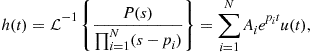
The inverse Laplace transform is given by
![]() (2.60)
(2.60)
The integration is performed along a line, parallel to the imaginary axis, (![]() ) that lies in the ROC. However, the inverse transform can be calculated using partial fractions expansion with the method of residues. In this method, the s-domain signal
) that lies in the ROC. However, the inverse transform can be calculated using partial fractions expansion with the method of residues. In this method, the s-domain signal ![]() is decomposed into partial fractions, thus expressing
is decomposed into partial fractions, thus expressing ![]() as a sum of simpler rational functions. Hence, as each term in the partial fraction is expected to have a known inverse transform, each transform may be obtained from a table like Table 2.2. Please recall that the ROC of a signal that is non-zero for
as a sum of simpler rational functions. Hence, as each term in the partial fraction is expected to have a known inverse transform, each transform may be obtained from a table like Table 2.2. Please recall that the ROC of a signal that is non-zero for ![]() is located to the right hand side of its poles. Conversely, for a signal that is non-zero for
is located to the right hand side of its poles. Conversely, for a signal that is non-zero for ![]() , the ROC of its Laplace transform lies to the left-hand side of its poles. In other words, if
, the ROC of its Laplace transform lies to the left-hand side of its poles. In other words, if ![]() , its inverse Laplace transform is given as follows:
, its inverse Laplace transform is given as follows:
 (2.61)
In practice, the inverse Laplace transform is found recursing to tables of transform pairs (e.g., Table 2.2). Given a function ![]() in the s-domain and a region of convergence, its inverse Laplace transform is given by
in the s-domain and a region of convergence, its inverse Laplace transform is given by ![]() such that
such that ![]() .
.
An immediate application of the Laplace transform is on circuit analysis. Assuming that all initial conditions are equal to zero, i.e., there is no initial charge on the capacitor, the response ![]() of the circuit with input given by
of the circuit with input given by ![]() displayed by Figure 2.4 could be obtained in the Laplace domain to be further transformed into the time-domain.
displayed by Figure 2.4 could be obtained in the Laplace domain to be further transformed into the time-domain.
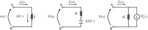
First, the circuit elements are transformed from the time domain into the s-domain, thus creating an s-domain equivalent circuit. Hence, the RLC elements in the time domain and s-domain are:Resistor (voltage-current relationship):
![]() (2.62)
(2.62)
The equivalent circuit is depicted in Figure 2.12.Inductor (initial current ![]() ):
):
![]() (2.63)
(2.63)
applying the differentiation property (Table 2.3) leads to
![]() (2.64)
(2.64)

The equivalent circuit is depicted in Figure 2.13. The inductor, L, is an impedance sL in the s-domain in series with a voltage source, ![]() , or in parallel with a current source,
, or in parallel with a current source, ![]() .Capacitor (initial voltage
.Capacitor (initial voltage ![]() ):
):
![]() (2.65)
(2.65)
applying the differentiation property (Table 2.3) leads to
![]() (2.66)
(2.66)
The capacitor, C, is an impedance ![]() in the s-domain in series with a voltage source,
in the s-domain in series with a voltage source, ![]() , or in parallel with a current source,
, or in parallel with a current source, ![]() . The voltage across the capacitor in the time-domain corresponds to the voltage across both the capacitor and the voltage source in the frequency domain. As an example, the system’s response given by the voltage across the capacitor,
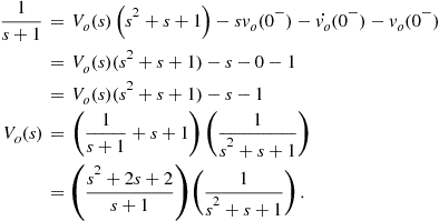
. The voltage across the capacitor in the time-domain corresponds to the voltage across both the capacitor and the voltage source in the frequency domain. As an example, the system’s response given by the voltage across the capacitor, ![]() , depicted in Figure 2.4, is obtained in the Laplace domain as follows (see Figure 2.14):
, depicted in Figure 2.4, is obtained in the Laplace domain as follows (see Figure 2.14):
![]() (2.67)
(2.67)

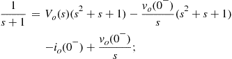
From (2.65), we have
![]() (2.68)
(2.68)
![]() (2.69)
(2.69)
Substituting (2.69) in (2.68) and applying the inverse Laplace transform (Table 2.2) and and the linearity property (Table 2.3), we get
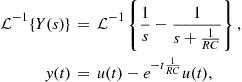 (2.70)
which is the same result presented in (2.5).
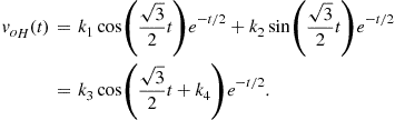
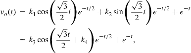
Another example, where the Laplace transform is useful, is the RLC circuit displayed by Figure 2.8 where the desired response is the voltage across the capacitor ![]() . Note that the initial conditions are part of the transform, as well as the transient and steady-state responses. Given the input signal
. Note that the initial conditions are part of the transform, as well as the transient and steady-state responses. Given the input signal ![]() with initial conditions
with initial conditions ![]() , and
, and ![]() , applying the Kirchhoff’s voltage law to the circuit, we have:
, applying the Kirchhoff’s voltage law to the circuit, we have:
![]() (2.71)
(2.71)
Directly substituting (2.62), (2.63) and (2.65) in (2.71), and applying the Laplace transform to the input signal, ![]() , we get
, we get
 (2.72)
which, from (2.65), ![]() , we have
, we have
 (2.73)
Substituting the values of ![]() (in
(in ![]() ),
), ![]() (in H),
(in H), ![]() (in F), the equation becomes
(in F), the equation becomes
 (2.74)
considering that the initial conditions are ![]() , we get
, we get
 (2.75)
After decomposing (2.75) into partial fractions and finding the poles and residues, the inverse Laplace transform is applied in order to find the expression of ![]() :
:
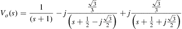 (2.76)
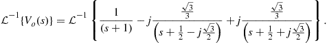 (2.77)
Applying the linearity property (Table 2.3) and and recursing to the Laplace transform pair table (Table 2.2), we get
![]() (2.78)
(2.78)
considering that the inverse Laplace transforms of ![]() , for
, for ![]() , given by Table 2.2, with
, given by Table 2.2, with ![]() and
and ![]() are
are

respectively.
Algebraically manipulating (2.78) and substituting the terms of complex exponentials by trigonometric identities, we have (for ![]() )
)
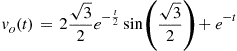 (2.79)
![]()
The solution given by (2.79) in the same given by (2.33). However, in the solution obtained using the Laplace transform, the initial conditions were part of the transform. We could also have applied the Laplace transform directly to the ODE (2.30) assisted by Tables 2.3 and 2.2, as follows:
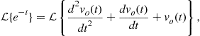 (2.80)
where
 (2.81)
Hence, substituting the expressions from (2.81) into (2.80) and considering the initial conditions, we obtain the same final expression presented in (2.75):
 (2.82)
In Section 1.02.2 the importance of working with a LTI system was introduced. The convolution integral in (2.9), that expresses the input signal, ![]() , as a sum of scaled and shifted impulse functions, uses delayed unit impulses as its basic signals. Therefore, a LTI system response is the same linear combination of the responses to the basic inputs.
, as a sum of scaled and shifted impulse functions, uses delayed unit impulses as its basic signals. Therefore, a LTI system response is the same linear combination of the responses to the basic inputs.
Considering that complex exponentials, such as ![]() , are eigensignals of LTI systems, Eq. (2.36) is defined if one uses
, are eigensignals of LTI systems, Eq. (2.36) is defined if one uses ![]() as a basis for the set of all input functions in a linear combination made of infinite terms (i.e., an integral). As the signal is being decomposed in basic inputs (complex exponentials), the LTI system’s response could be characterized by weighting factors applied to each component in that representation.
as a basis for the set of all input functions in a linear combination made of infinite terms (i.e., an integral). As the signal is being decomposed in basic inputs (complex exponentials), the LTI system’s response could be characterized by weighting factors applied to each component in that representation.
In Section 1.02.7, the Fourier transform is introduced and it is shown that the Fourier integral does not converge for a large class of signals. The Fourier transform may be considered a subset of the Laplace transform, or the Laplace transform could be considered a generalization (or expansion) of the Fourier transform. The Laplace integral term ![]() , from (2.36), forces the product
, from (2.36), forces the product ![]() to zero as time t increases. Therefore, it could be regarded as the exponential weighting term that provides convergence to functions for which the Fourier integral does not converge.
to zero as time t increases. Therefore, it could be regarded as the exponential weighting term that provides convergence to functions for which the Fourier integral does not converge.
Following the concept of representing signals as a linear combination of eigensignals, instead of choosing ![]() as the eigensignals, one could choose
as the eigensignals, one could choose ![]() as the eigensignals. The latter representation leads to the Fourier transform equation, and any LTI system’s response could be characterized by the amplitude scaling applied to each of the basic inputs
as the eigensignals. The latter representation leads to the Fourier transform equation, and any LTI system’s response could be characterized by the amplitude scaling applied to each of the basic inputs ![]() . Laplace transform and applications are discussed in greater detail in [2,4,5,8,1011].
. Laplace transform and applications are discussed in greater detail in [2,4,5,8,1011].
1.02.5 Transfer function and stability
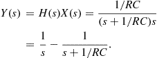
The Laplace transform, seen in the previous section, is an important tool to solve differential equations and therefore to obtain, once given the input, the output of a linear and time invariant (LTI) system. For a LTI system, the Laplace transform of its mathematical representation, given as a differential equation—with constant coefficients and null initial conditions—as in (2.22) or, equivalently, given by a convolution integral as in (2.10), leads to the concept of transfer function, the ratio
![]() (2.83)
(2.83)
between the Laplace transform of the output signal and the Laplace transform of the input signal. This representation of a LTI system also corresponds to the Laplace transform of its impulse response, i.e., ![]() .
.
Assuming that all initial conditions are equal to zero, solving a system using the concept of transfer function is usually easier for the convolution integral is replaced by a multiplication in the transformed domain:
![]() (2.84)
(2.84)
such that
![]() (2.85)
(2.85)
the zero-state response of this system.
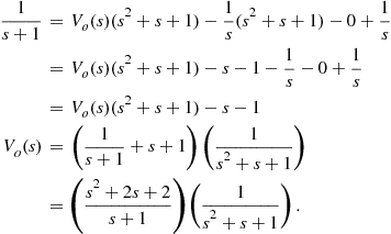
A simple example is given from the circuit in Figure 2.4 where
![]()
If ![]() , and
, and
Therefore, ![]() corresponds to
corresponds to
![]()
which is the same solution given in (2.5).
Given (2.10) and provided that all initial conditions are null, the transfer function ![]() corresponds to a ratio of two polynomials in s:
corresponds to a ratio of two polynomials in s:
![]() (2.86)
(2.86)
The roots of the numerator ![]() are named zeros while the roots of the denominator
are named zeros while the roots of the denominator ![]() are known as poles. Both are usually represented in the complex plane
are known as poles. Both are usually represented in the complex plane ![]() and this plot is referred to as pole-zero plot or pole-zero diagram.
and this plot is referred to as pole-zero plot or pole-zero diagram.
We use the ODE (2.29) to provide an example:
![]() (2.87)
(2.87)
Using the same values, ![]() (in
(in ![]() ),
), ![]() (in H),
(in H), ![]() (in F), we obtain the poles (roots of the characteristic equation)
(in F), we obtain the poles (roots of the characteristic equation) ![]() as seen in Figure 2.15.
as seen in Figure 2.15.

Figure 2.15 An example of a pole-zero diagram of the transfer function in (2.87) for ![]() (in
(in ![]() ),
), ![]() (in H),
(in H), ![]() (in F). The gray curve corresponds to the root-locus of the poles when R varies from
(in F). The gray curve corresponds to the root-locus of the poles when R varies from ![]() (poles at
(poles at ![]() ) to
) to ![]() (poles at
(poles at ![]() and at
and at ![]() ). See refgroup Refmmcvideo4Video 4 to watch animation.
). See refgroup Refmmcvideo4Video 4 to watch animation.
For a LTI system, a complex exponential ![]() can be considered an eigensignal:
can be considered an eigensignal:
 (2.88)
which is valid only for those values of s where ![]() exists.
exists.
If there is no common root between ![]() and
and ![]() , the denominator of
, the denominator of ![]() corresponds to the characteristic polynomial and, therefore, poles
corresponds to the characteristic polynomial and, therefore, poles ![]() of a LTI system correspond to their natural frequencies.
of a LTI system correspond to their natural frequencies.
As mentioned in Section 1.02.2, the stability of a system, in a bounded-input bounded-output (BIBO) sense, implies that if ![]() then
then ![]() and
and ![]() , for all values of t. This corresponds to its input response being absolutely integrable, i.e.,
, for all values of t. This corresponds to its input response being absolutely integrable, i.e.,
![]() (2.89)
(2.89)
As seen previously, the natural response of a linear system corresponds to a linear combination of complex exponentials ![]() . Let us assume, for convenience, that
. Let us assume, for convenience, that ![]() has N distinct poles and that the order of
has N distinct poles and that the order of ![]() is lower than the order of
is lower than the order of ![]() ; in that case, we can write
; in that case, we can write
 (2.90)
where constants ![]() are obtained from simple partial fraction expansion.
are obtained from simple partial fraction expansion.
In order for the system to be stable, each exponential should tend to zero as t tends to zero. Considering a complex pole ![]() should imply that
should imply that ![]() or
or ![]() ; that is, the real part of
; that is, the real part of ![]() should be negative.
should be negative.
While the location of the zeros of ![]() is irrelevant for the stability of a LTI system, their poles are of paramount importance. We summarize this relationship in the following:
is irrelevant for the stability of a LTI system, their poles are of paramount importance. We summarize this relationship in the following:
1. A causal LTI system is BIBO stable if and only if all poles of its transfer function have negative real part (belong to the left-half of the s-plane).
2. A causal LTI system is unstable if and only if at least one of the following conditions occur: one pole of ![]() has a positive real part and repeated poles of
has a positive real part and repeated poles of ![]() have real part equal to zero (belong to the imaginary axis of the s-plane).
have real part equal to zero (belong to the imaginary axis of the s-plane).
3. A causal LTI system is marginally stable if and only if there are no poles on the right-half of the s-plane and non-repeated poles occur on its imaginary axis.
We can also state system stability from the region of convergence of ![]() : a LTI system is stable if and only if the ROC of
: a LTI system is stable if and only if the ROC of ![]() includes the imaginary axis (
includes the imaginary axis (![]() ). Figure 2.16 depicts examples of impulse response for BIBO stable, marginally stable, and unstable systems.
). Figure 2.16 depicts examples of impulse response for BIBO stable, marginally stable, and unstable systems.

Figure 2.16 Pole location on the s-plane and system stability: examples of impulse responses of causal LTI systems. Visit the “exploring the s-plane” http://www.jhu.edu/signals/explore/index.html website.
In this section, we have basically addressed BIBO stability which, although not sufficient for asymptotic stability (a system can be BIBO stable without being stable when initial conditions are not null), is usually employed for linear systems. A more thorough stability analysis could be carried out by using Lyapunov criteria [13].
The Laplace transform applied to the input response of the differential equation provides the transfer function which poles (roots of its denominator) determines the system stability: a causal LTI system is said to be stable when all poles lie in the left half of the complex s-plane. In this case, the system is also known as asymptotically stable for its output always tend to decrease, not presenting permanent oscillation.
Whenever distinct poles have their real part equal to zero (poles on the imaginary axis), permanent oscillation will occur and the system is marginally stable, the output signal does not decay nor grows indefinitely. Figure 2.16 shows the impulse response growing over time when two repeated poles are located on the imaginary axis. Although not shown in Figure 2.16, decaying exponential will take place of decaying oscillation when poles are real (and negative) while growing exponentials will appear for the case of real positive poles.
Although we have presented the key concepts of stability related to a linear system, much more could be said about stability theory. Hence, further reading is encouraged: [2,13].
1.02.6 Frequency response
We have mentioned in the previous section that the complex exponential ![]() is an eigensignal of a continuous-time linear system. A particular choice of s being
is an eigensignal of a continuous-time linear system. A particular choice of s being ![]() , i.e., the input signal
, i.e., the input signal
![]() (2.91)
(2.91)
has a single frequency and the output, from (2.88), is
 (2.92)
Being ![]() an eigensignal,
an eigensignal, ![]() in (2.92) corresponds to its eigenvalue. Allowing a variable frequency
in (2.92) corresponds to its eigenvalue. Allowing a variable frequency ![]() instead of a particular value
instead of a particular value ![]() , we define the frequency response of a linear system having impulse response
, we define the frequency response of a linear system having impulse response ![]() as
as
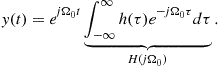
![]() (2.93)
(2.93)
We note that the frequency response corresponds to the Laplace transform of ![]() on a specific region of the s-plane, the vertical (or imaginary) axis
on a specific region of the s-plane, the vertical (or imaginary) axis ![]() :
:
![]() (2.94)
(2.94)
It is clear from (2.93) that the frequency response ![]() of a linear system is a complex function of
of a linear system is a complex function of ![]() . Therefore, it can be represented in its polar form as
. Therefore, it can be represented in its polar form as
![]() (2.95)
(2.95)
As an example, we use the RLC series circuit given in Figure 2.17 with ![]() (in H),
(in H), ![]() (in F), and R varying from
(in F), and R varying from ![]() to
to ![]() (in
(in ![]() ).
).

Figure 2.17 RLC series circuit: the transfer function is ![]() ,
, ![]() and
and ![]() , and the frequency response is given by
, and the frequency response is given by ![]() .
.
The frequency response, magnitude or absolute value (in dB) and argument or phase (in radians), are depicted in Figure 2.18. For this example, we consider the voltage applied to the circuit as input and the voltage measured at the capacitor as output. This is worth mentioning since the output could be, for instance, the current in the circuit or the voltage across the inductor.
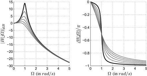
Figure 2.18 Frequency response in magnitude (![]() in dB) and normalized phase (argument of
in dB) and normalized phase (argument of ![]() divided by
divided by ![]() , i.e.,
, i.e., ![]() corresponds to
corresponds to ![]() ) for the circuit in Figure 2.17 with
) for the circuit in Figure 2.17 with ![]() (in H),
(in H), ![]() (in F), and R varying from 0.2 (in
(in F), and R varying from 0.2 (in ![]() ) (highlighted highest peak in magnitude) to 1.2 (in
) (highlighted highest peak in magnitude) to 1.2 (in ![]() ). Download the http://www.ime.eb.br/∼apolin/CTSS/Figs18and19.m Matlab© code.
). Download the http://www.ime.eb.br/∼apolin/CTSS/Figs18and19.m Matlab© code.
In low frequencies, the capacitor tends to become an open circuit such that ![]() and the gain tends to 1 or 0 dB. On the other hand, as the frequency
and the gain tends to 1 or 0 dB. On the other hand, as the frequency ![]() goes towards infinity, the capacitor tends to become a short circuit such that
goes towards infinity, the capacitor tends to become a short circuit such that ![]() goes to zero, gain in dB tending to minus infinity. The circuit behaves like a low-pass filter allowing low frequencies to the output while blocking high frequencies. Specially, when R has low values (when tending to zero), we observe a peak in
goes to zero, gain in dB tending to minus infinity. The circuit behaves like a low-pass filter allowing low frequencies to the output while blocking high frequencies. Specially, when R has low values (when tending to zero), we observe a peak in ![]() at
at ![]() . This frequency,
. This frequency, ![]() , is termed the resonance frequency and corresponds to the absolute value of the pole responsible for this oscillation.
, is termed the resonance frequency and corresponds to the absolute value of the pole responsible for this oscillation.
Let us write the frequency response from ![]() , as given in (2.87):
, as given in (2.87):
![]() (2.96)
(2.96)
We note that, when ![]() , the peak amplitude of
, the peak amplitude of ![]() occurs for
occurs for ![]() (it tends to infinity as R goes to zero), i.e., the resonance frequency corresponds to
(it tends to infinity as R goes to zero), i.e., the resonance frequency corresponds to ![]() .
.
The impulse response as well as the pole diagram are shown in Figure 2.19; from this figure, we observe the oscillatory behavior of the circuit as R tends to zero in both time- and s-domain (poles approaching the vertical axis). The impulse response and the poles location for the minimum value of the resistance, ![]() (in
(in ![]() )), are highlighted in this figure.
)), are highlighted in this figure.

Figure 2.19 Impulse responses and poles location in the s-plane (6 different values of R) for the circuit in Figure 2.17. Note that, for lower values of ![]() tends to oscillate and the poles are closer to the vertical axis (marginal stability region). Download the http://www.ime.eb.br/∼apolin/CTSS/Figs18and19.m Matlab© code.
tends to oscillate and the poles are closer to the vertical axis (marginal stability region). Download the http://www.ime.eb.br/∼apolin/CTSS/Figs18and19.m Matlab© code.
Before providing more details about the magnitude plot of the frequency response as a function of ![]() , let us show the (zero state) response of a linear system to a real single frequency excitation
, let us show the (zero state) response of a linear system to a real single frequency excitation ![]() . We know that the complex exponential is an eigensignal to a linear system such that, making
. We know that the complex exponential is an eigensignal to a linear system such that, making ![]() ,
,
![]() (2.97)
(2.97)
Since we can write ![]() as
as ![]() , the output shall be given as
, the output shall be given as
![]() (2.98)
(2.98)
Assuming that ![]() is real, it is possible to assure that all poles of
is real, it is possible to assure that all poles of ![]() will occur in complex conjugate pairs, leading (as shall be also addressed in the next section) to
will occur in complex conjugate pairs, leading (as shall be also addressed in the next section) to ![]() . This conjugate symmetry property of the frequency response, i.e.,
. This conjugate symmetry property of the frequency response, i.e., ![]() and
and ![]() , when applied in (2.98), results in
, when applied in (2.98), results in
![]() (2.99)
(2.99)
The previous expression is also valid as regime solution when the input is a sinusoid, that is non-zero for ![]() , such as
, such as ![]() .
.
Now, back to our example of a frequency response given in (2.96), let us express its magnitude squared:
![]() (2.100)
(2.100)
It is easy to see that, when ![]() tends to zero, the magnitude squared tends to one while, when
tends to zero, the magnitude squared tends to one while, when ![]() tends to infinity, the dominant term becomes
tends to infinity, the dominant term becomes ![]() :
:
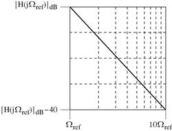
These two regions of ![]() , close to zero and tending to infinity, could be visualized by lines in a semi-log plot, the frequency axis, due to its large range of values, is plotted using a logarithmic scale. Particularly, when
, close to zero and tending to infinity, could be visualized by lines in a semi-log plot, the frequency axis, due to its large range of values, is plotted using a logarithmic scale. Particularly, when ![]() , the approximation in (b) tells us that, in an interval from
, the approximation in (b) tells us that, in an interval from ![]() to
to ![]() (the resonance frequency), we have an attenuation of 40 dB as shown in Figure 2.20.
(the resonance frequency), we have an attenuation of 40 dB as shown in Figure 2.20.
Magnitude in dB and phase of ![]() as a function of
as a function of ![]() , plotted in a logarithmic frequency scale, is known as Bode Plots or Bode Diagrams. A Bode Diagram may be sketched from lines (asymptotes) which are drawn from the structure of
, plotted in a logarithmic frequency scale, is known as Bode Plots or Bode Diagrams. A Bode Diagram may be sketched from lines (asymptotes) which are drawn from the structure of ![]() , its poles and zeros. For the case of a transfer function with two conjugate complex roots, we have
, its poles and zeros. For the case of a transfer function with two conjugate complex roots, we have
![]() (2.101)
(2.101)
where, in our example in (2.87), ![]() and
and ![]() . Also note that (in order to have two conjugate complex roots)
. Also note that (in order to have two conjugate complex roots) ![]() .
.
The magnitude of the frequency response in dB is given as
 (2.102)
When ![]() ; this value being a good approximation for the peak magnitude (see Figure 2.21) when
; this value being a good approximation for the peak magnitude (see Figure 2.21) when ![]() tends to zero (we have an error lower than 0.5% when
tends to zero (we have an error lower than 0.5% when ![]() ). The peak actually occurs in
). The peak actually occurs in ![]() , having a peak height equal to
, having a peak height equal to ![]() ; we could also add that the peak is basically observable only when
; we could also add that the peak is basically observable only when ![]() . The Bode Plot of (2.87), with
. The Bode Plot of (2.87), with ![]() (in
(in ![]() ),
), ![]() (in H), and
(in H), and ![]() (in F) showing the (low frequency and high frequency) asymptotes is depicted in Figure 2.21.
(in F) showing the (low frequency and high frequency) asymptotes is depicted in Figure 2.21.

Figure 2.21 Example of Bode Plot for ![]() with
with ![]() and
and ![]() . Note that, for this case, the approximated height of the peak
. Note that, for this case, the approximated height of the peak ![]() works well.
works well.
Another example with first order poles and zeros will end our discussion on Bode Plots. Let transfer function ![]() , with poles at −1 and −10,000, and zeros at −10 and −1000, be represented as follows:
, with poles at −1 and −10,000, and zeros at −10 and −1000, be represented as follows:
 (2.103)
The magnitude in dB of its frequency response could then be written as
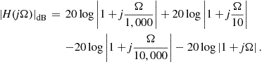 (2.104)
The first term, as in the previous example, can be checked for low and high frequencies:
When ![]() , the value of this term is
, the value of this term is ![]() which is the usual error at the these frequencies (cutoff frequencies).
which is the usual error at the these frequencies (cutoff frequencies).
We could, from the analysis of the first term, extend the results to all cutoff frequencies as shown in Table 2.4. The resulting asymptotic sketch and real curves are shown in Figure 2.22 where we observe the 3 dB errors at the cutoff frequencies.
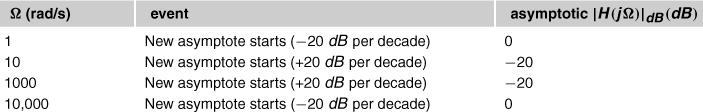
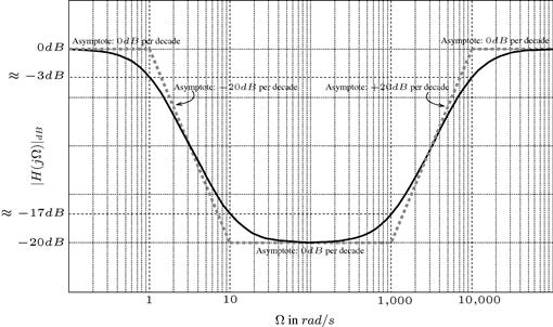
Figure 2.22 Bode Magnitude (dB) Plot for ![]() . Download the http://www.ime.eb.br/∼apolin/CTSS/Fig22.m Matlab© code.
. Download the http://www.ime.eb.br/∼apolin/CTSS/Fig22.m Matlab© code.
A final observation is regarded to the phase of the frequency response: similarly to the magnitude, a sketch of the phase can also be obtained from the poles and zeros of ![]() :
:
![]() (2.105)
(2.105)
The first term on the right hand side of (2.105),![]() , can be checked for low and high frequencies:
, can be checked for low and high frequencies:
Considering only this zero (corresponding cutoff frequency ![]() ), one may assume
), one may assume ![]() and
and ![]() sufficiently small and sufficiently large such that an asymptote could be drawn between points
sufficiently small and sufficiently large such that an asymptote could be drawn between points ![]() and
and ![]() as in Figure 2.23. For a pole, the asymptote is mirrored with respect to
as in Figure 2.23. For a pole, the asymptote is mirrored with respect to ![]() .
.
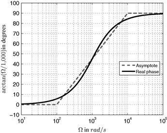
The asymptotic sketch and real phase curves for (2.105) is shown in Figure 2.24; note that we have two negative slope asymptotes, starting in ![]() and
and ![]() , and two positive slope asymptotes, starting at
, and two positive slope asymptotes, starting at ![]() and
and ![]() .
.
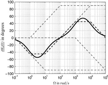
Figure 2.24 Bode Phase Plot for ![]() . Lighter gray dashed lines represent the asymptotes and the darker dashed line corresponds to the asymptotic sketch (sum of the asymptotes); the real phase is the continuous curve in black. Download the http://www.ime.eb.br/∼apolin/CTSS/Fig24.m Matlab© code.
. Lighter gray dashed lines represent the asymptotes and the darker dashed line corresponds to the asymptotic sketch (sum of the asymptotes); the real phase is the continuous curve in black. Download the http://www.ime.eb.br/∼apolin/CTSS/Fig24.m Matlab© code.
The topics discussed in this section are found in the following books: [1,3,8,14,15].
1.02.7 The Fourier series and the Fourier transform
In electronic circuits we often deal with periodic and non-periodic signals. In addition, circuits could be driven by non-sinusoidal functions. Hence, methods that decompose continuous-time periodic (non-sinusoidal) and non-periodic signals into contributions from sinusoidal (![]() and
and ![]() ) signals are extremely valuable for electronic system analysis; this is due to the fact that a LTI system only changes the amplitude and phase of a real sinusoid. Several properties make sinusoids an ideal choice to be the elementary basis functions for signal analysis and synthesis. For example, Eq. (2.99) shows that the LTI system changed the amplitude to
) signals are extremely valuable for electronic system analysis; this is due to the fact that a LTI system only changes the amplitude and phase of a real sinusoid. Several properties make sinusoids an ideal choice to be the elementary basis functions for signal analysis and synthesis. For example, Eq. (2.99) shows that the LTI system changed the amplitude to ![]() and the phase to
and the phase to ![]() of the given sinusoidal input,
of the given sinusoidal input, ![]() . In addition, as sine and cosine are mutually orthogonal, sinusoidal basis functions are independent and can be processed independently. Usually, any sinusoidal function, such as the one mentioned above, can be expressed as a linear combination of sine and cosine functions:
. In addition, as sine and cosine are mutually orthogonal, sinusoidal basis functions are independent and can be processed independently. Usually, any sinusoidal function, such as the one mentioned above, can be expressed as a linear combination of sine and cosine functions: ![]() . If a signal is a sum of sinusoids, such as
. If a signal is a sum of sinusoids, such as
![]() (2.106)
(2.106)
its impulse response, considering it is a linear system, would be given by
![]() (2.107)
(2.107)
A periodic signal, ![]() , with period T, may contain components at frequencies
, with period T, may contain components at frequencies ![]() , where the fundamental frequency is given by
, where the fundamental frequency is given by ![]() . The frequencies
. The frequencies ![]() are the harmonics, and any pair of signals are harmonically related if their periods are related by a integer ratio. In general, the resulting signal from a sum of harmonically related waveforms is also periodic, and its repetition period is equal to the fundamental period. The harmonic components exist only at discrete frequencies.
are the harmonics, and any pair of signals are harmonically related if their periods are related by a integer ratio. In general, the resulting signal from a sum of harmonically related waveforms is also periodic, and its repetition period is equal to the fundamental period. The harmonic components exist only at discrete frequencies.
Consider that we add the harmonically related signals, ![]() , with
, with ![]() , over
, over ![]() such that
such that ![]() , and get
, and get ![]() as the result when
as the result when ![]() and when
and when ![]() , meaning that infinite terms are added:
, meaning that infinite terms are added:
 (2.108)
The resulting waveforms, ![]() for
for ![]() and
and ![]() when N is large, i.e.,
when N is large, i.e., ![]() , are displayed by Figure 2.25. It is clear that as the number of terms becomes infinite in (2.108) the result converges at every value of the period T (to the square wave) except at the discontinuities. Actually, the ringing effect at the discontinuities (not shown in Figure 2.25 for the curve with the large value of N) never dies out as N becomes larger, yet reaching a finite limit (Gibbs phenomenon).
, are displayed by Figure 2.25. It is clear that as the number of terms becomes infinite in (2.108) the result converges at every value of the period T (to the square wave) except at the discontinuities. Actually, the ringing effect at the discontinuities (not shown in Figure 2.25 for the curve with the large value of N) never dies out as N becomes larger, yet reaching a finite limit (Gibbs phenomenon).
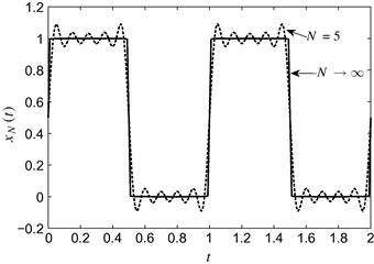
Figure 2.25 Synthesized square wave from Eq. (2.108).
Hence, for a period T, for a fundamental frequency ![]() with frequencies that are integer multiples of the fundamental frequency such that
with frequencies that are integer multiples of the fundamental frequency such that ![]() (the set of all integers), the representation of the harmonic components,
(the set of all integers), the representation of the harmonic components, ![]() , of a signal
, of a signal ![]() can be written as
can be written as
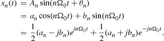 (2.109)
Equation (2.109) presents three equivalent forms to express the harmonic components ![]() : the first one is written as a sine function with amplitude
: the first one is written as a sine function with amplitude ![]() and phase
and phase ![]() ; the second one as sum of sine and cosine functions with real coefficients
; the second one as sum of sine and cosine functions with real coefficients ![]() and
and ![]() , respectively; and the last form writes
, respectively; and the last form writes ![]() in terms of complex exponentials.
in terms of complex exponentials.
The derivation, providing proofs, of the expressions for computing the coefficients in a Fourier series is beyond the scope of this chapter. Hence, we simply state, without proof, that if ![]() is periodic with period T and fundamental frequency
is periodic with period T and fundamental frequency ![]() , any arbitrary real periodic signal
, any arbitrary real periodic signal ![]() could be represented by the infinite summation of harmonically related sinusoidal components, known as the Fourier series:
could be represented by the infinite summation of harmonically related sinusoidal components, known as the Fourier series:
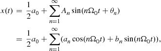 (2.110)
where for ![]() , we have the term
, we have the term ![]() corresponding to the mean value of the signal, with frequency of 0 Hz, known as the DC value (or level), and the other terms are as follows:
corresponding to the mean value of the signal, with frequency of 0 Hz, known as the DC value (or level), and the other terms are as follows:
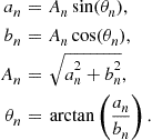 (2.111)
If in the last form presented in (2.109), we substitute
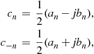 (2.112)
to have a third representation of the Fourier series, given by
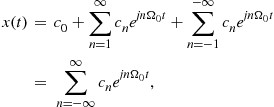 (2.113)
where ![]() is real and
is real and ![]() are complex, for
are complex, for ![]() , coefficients. The coefficients of terms for positive (
, coefficients. The coefficients of terms for positive (![]() ) and negative (
) and negative (![]() ) values of n are complex conjugates (
) values of n are complex conjugates (![]() ). This Fourier series form demands the summation to be performed over all
). This Fourier series form demands the summation to be performed over all ![]() , as the continuous-time complex sinusoids,
, as the continuous-time complex sinusoids, ![]() , present an infinite number of terms (specific frequencies
, present an infinite number of terms (specific frequencies ![]() ). Moreover, for every integer value of n,
). Moreover, for every integer value of n, ![]() is periodic with
is periodic with ![]() . Hence, the periodic signal
. Hence, the periodic signal ![]() must have
must have ![]() in order to compute the Fourier series expansion. However, the analysis of the Fourier cosine series of a function x in the interval
in order to compute the Fourier series expansion. However, the analysis of the Fourier cosine series of a function x in the interval ![]() is equivalent to the analysis of its extension first to
is equivalent to the analysis of its extension first to ![]() as an even function, then to all of components with period
as an even function, then to all of components with period ![]() .
.
The complex exponential representation of the Fourier series, given by (2.113) generates a two-sided spectrum, as the summation requires all ![]() . The first and second representations of the Fourier series, presented in (2.110) produce a one-sided spectra, as the sum is computed only for values of
. The first and second representations of the Fourier series, presented in (2.110) produce a one-sided spectra, as the sum is computed only for values of ![]() .
.
Equations (2.110) and (2.113) are called Fourier synthesis equations as it is possible to synthesize any periodic (time) signal, ![]() , from an infinite set of harmonically related signals.
, from an infinite set of harmonically related signals.
If ![]() is periodic with fundamental frequency
is periodic with fundamental frequency ![]() and period T, the coefficients of the three Fourier series equivalent representations are given by
and period T, the coefficients of the three Fourier series equivalent representations are given by
![]() (2.114)
(2.114)
and by manipulating (2.112) we obtain
 (2.115)
where the integrals in (2.114) and (2.115) are obtained over any interval that corresponds to the period T, with the initial time ![]() for the integration arbitrarily defined.
for the integration arbitrarily defined.
Equations (2.114) and (2.115) are known as Fourier analysis or Fourier decomposition as the signal is being decomposed into its spectral components (basic inputs).
The continuous-time Fourier series expands any continuous-time periodic signal into a series of sine waves. The Fourier analysis methods are named after the French mathematician Jean-Baptiste Joseph Fourier. In general, almost any periodic signal can be written as an infinite sum of complex exponential functions (or real sinusoidal functions) and thus be represented as a Fourier series. Therefore, finding the response to a Fourier series, means finding the response to any periodic function, and its effect on its spectrum. When computing trigonometric coefficients, one could multiply a random signal by sinusoids of different frequencies to disclose all the (hidden) frequency components of the signal. In this way, it becomes easier to isolate the signal of the television station we want to watch from the others that are being simultaneously received by our television set.
In addition, the multiplication of a signal by ![]() means that the signal if being frequency shifted to
means that the signal if being frequency shifted to ![]() . Which is equivalent to the Frequency Shift Laplace Property (Table 2.3).
. Which is equivalent to the Frequency Shift Laplace Property (Table 2.3).
Consider ![]() , where
, where ![]() is the DC level, and three non-null harmonics (
is the DC level, and three non-null harmonics (![]() ) with the time-domain representation displayed by Figure 2.1. The signal has several (hidden) frequencies, and no clue is provided when visually inspecting Figure 2.1. The Fourier series representations are very helpful in this case, showing the amplitudes and phases of each harmonic in the frequency-domain.
) with the time-domain representation displayed by Figure 2.1. The signal has several (hidden) frequencies, and no clue is provided when visually inspecting Figure 2.1. The Fourier series representations are very helpful in this case, showing the amplitudes and phases of each harmonic in the frequency-domain.
The exponential form, recursing to trigonometric identities, is given by:
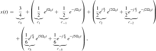 (2.116)
and the Fourier series exponential form coefficients are (all other terms are zero).
The complex-valued coefficient ![]() conveys both the amplitude (
conveys both the amplitude (![]() ) and phase
) and phase ![]() of the frequency content of the signal
of the frequency content of the signal ![]() at each value
at each value ![]() rad/s as pictured in (Figure 2.26).
rad/s as pictured in (Figure 2.26).
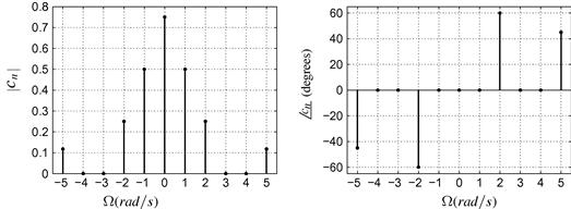
Figure 2.26 Two-sided spectrum of periodic signal ![]() depicted in Figure 2.1.
depicted in Figure 2.1.
The sinusoidal basis functions of the Fourier series are smooth and infinitely differentiable but they only represent periodic signals. The Fourier representation for a non-periodic (time-domain) signal has to treat the frequency spectrum of non-periodic signals as a continuous function of frequency. This representation could be obtained by considering a non-periodic signal as a special case of a periodic signal with an infinite period. The idea is that if the period of a signal is infinite (![]() ), then it is never repeated. Hence, it is non-periodic. As
), then it is never repeated. Hence, it is non-periodic. As ![]() , thus decreasing the spacing between each adjacent line spectra (representing each harmonic contribution in the spectrum) towards a continuous representation of frequency.
, thus decreasing the spacing between each adjacent line spectra (representing each harmonic contribution in the spectrum) towards a continuous representation of frequency.
The generalization to non-periodic signals is known as the Fourier transform and is given by (2.117). It is analogous to the Fourier series analysis Eq. (2.114). It expresses the time-domain function ![]() as a continuous function of frequency
as a continuous function of frequency ![]() defined as follows:
defined as follows:
![]() (2.117)
(2.117)
The inverse Fourier transform is analogous to the Fourier series synthesis equation (2.113). It obtains the time-domain signal, ![]() , from its frequency-domain representation
, from its frequency-domain representation ![]() :
:
![]() (2.118)
(2.118)
The notation ![]() denotes that
denotes that ![]() is the Fourier transform of
is the Fourier transform of ![]() . Conversely,
. Conversely, ![]() denotes that
denotes that ![]() is the inverse Fourier transform of
is the inverse Fourier transform of ![]() . This relationship is expressed with
. This relationship is expressed with ![]() .
.
The Fourier series coefficients have distinct units of amplitude, whereas ![]() has units of amplitude density. The magnitude of
has units of amplitude density. The magnitude of ![]() is termed as the magnitude spectrum (
is termed as the magnitude spectrum (![]() ) and its phase as the phase spectrum
) and its phase as the phase spectrum ![]() .
.
Following the concept of representing signals as a linear combination of eigensignals, instead of choosing ![]() as the eigensignals, one could choose
as the eigensignals, one could choose ![]() as the eigensignals. The latter representation leads to the Fourier transform equation, and any LTI system’s response could be characterized by the amplitude scaling applied to each of the basic inputs
as the eigensignals. The latter representation leads to the Fourier transform equation, and any LTI system’s response could be characterized by the amplitude scaling applied to each of the basic inputs ![]() .
.
This transform is very useful as it produces the frequency complex content of a signal, ![]() , from its temporal representation,
, from its temporal representation, ![]() . Moreover, the mapping provides a representation of the signal as combination of complex sinusoids (or exponentials) for frequency-domain behavior analysis, where the (computationally consuming) computation of the convolution in the time-domain is replaced by the (simple) operation of multiplication in the frequency-domain.
. Moreover, the mapping provides a representation of the signal as combination of complex sinusoids (or exponentials) for frequency-domain behavior analysis, where the (computationally consuming) computation of the convolution in the time-domain is replaced by the (simple) operation of multiplication in the frequency-domain.
Nevertheless, functions such as the unit-step (Figure 2.2a), discontinuous at time ![]() , does not have forward Fourier transform as its integral does not converge.
, does not have forward Fourier transform as its integral does not converge.
An analysis of convergence is beyond the scope of this chapter, hence we assume that the existence of the Fourier transform is assured by three (modified) Dirichlet conditions (for non-periodic signals), requiring the temporal signal, ![]() : to have a finite number of discontinuities, with the size of each discontinuity being finite; to have a finite number of local maxima an minima; and to be absolutely integrable, i.e.,
: to have a finite number of discontinuities, with the size of each discontinuity being finite; to have a finite number of local maxima an minima; and to be absolutely integrable, i.e.,
![]() (2.119)
(2.119)
These are sufficient conditions, although not strictly necessary as several common signals, such as the unit-step, are not absolutely integrable. Nevertheless, we can define a transform pair that satisfies the Fourier transform properties by the usage of impulses when dealing with this class of signals.
The Fourier transform converts a 1-D time-domain signal, ![]() , into its 1-D complex spectrum
, into its 1-D complex spectrum ![]() representation in frequency-domain. In Section 1.02.4, the Laplace transform maps a time-domain 1-D signal,
representation in frequency-domain. In Section 1.02.4, the Laplace transform maps a time-domain 1-D signal, ![]() , to a complex representation,
, to a complex representation, ![]() , defined over a complex plane (s-plane), spanned by its two variables
, defined over a complex plane (s-plane), spanned by its two variables ![]() and
and ![]() , as
, as ![]() . The Laplace and the Fourier transforms are closely related, when
. The Laplace and the Fourier transforms are closely related, when ![]() , i.e.,
, i.e., ![]() , the Laplace integral becomes the Fourier transform. Referring to Figure 2.10 (Section 1.02.4), as the imaginary axis (
, the Laplace integral becomes the Fourier transform. Referring to Figure 2.10 (Section 1.02.4), as the imaginary axis (![]() ) lies within the ROC, the Fourier transform exists only if
) lies within the ROC, the Fourier transform exists only if ![]() . For a certain class of signals, there is a simple relationship between the Fourier and the Laplace transforms given by
. For a certain class of signals, there is a simple relationship between the Fourier and the Laplace transforms given by
![]() (2.120)
(2.120)
The Laplace transform for ![]() is
is ![]() for
for ![]() (Table 2.2).
(Table 2.2). ![]() has a pole at
has a pole at ![]() , which lies at the left-half s-plane. The ROC is located at the right side of
, which lies at the left-half s-plane. The ROC is located at the right side of ![]() (right side of Figure 2.11), thus containing the imaginary axis (
(right side of Figure 2.11), thus containing the imaginary axis (![]() ) of the s-plane. Hence, the signal
) of the s-plane. Hence, the signal ![]() has a Fourier transform given by
has a Fourier transform given by ![]() . However, the Fourier transform does not converge for
. However, the Fourier transform does not converge for ![]() because
because ![]() is not absolutely integrable, whereas
is not absolutely integrable, whereas ![]() has a Laplace transform with the ROC pictured in the left side of Figure 2.11.
has a Laplace transform with the ROC pictured in the left side of Figure 2.11.
Common Fourier transform pairs are summarized in Table 2.5.
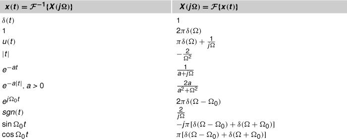
As the Laplace transform, the Fourier transform presents a set of properties. A comprehensive description of the properties of the Fourier transform is beyond the intent of this chapter, and the properties we examine are due to their importance in the study of electronic system analysis. Much of the usefulness of the Fourier transform arises from its properties, that have important interpretations in the context of continuous-time signal processing. Understanding the relationship between time- and frequency-domains (symmetry between operations) is a key point in the study (and usage) of the Fourier transform.(Time and frequency) scaling: If ![]() , then
, then ![]() , with
, with ![]() :
:
![]() (2.121)
(2.121)
 (2.122)
The two previous expressions can be combined in one single expression given by
 (2.123)
implying that a linear expansion of the time axis in the time-domain leads to linear compression of the frequency axis in the frequency-domain, and vice versa. This property indicates an important trade-off between the two domains, as narrow time-domain signals have wide Fourier representations (narrow pulses have wide bandwidth).Symmetry: The symmetry properties are quite useful as for a real-valued, a real-valued and even, a real-valued and odd, and an imaginary temporal signal, ![]() , we have the following relations:
, we have the following relations:

These properties are important as for a real-valued function in time its Fourier transform is conjugate symmetric, ![]() . This means that its real part (the magnitude) is an even function of frequency, and that its imaginary part (phase) is an odd function of frequency. Therefore, when we obtain the Fourier transform of a real-valued time function, it is only necessary to display the transform for positive values of
. This means that its real part (the magnitude) is an even function of frequency, and that its imaginary part (phase) is an odd function of frequency. Therefore, when we obtain the Fourier transform of a real-valued time function, it is only necessary to display the transform for positive values of ![]() . If the signal is even, i.e.,
. If the signal is even, i.e., ![]() , it has a Fourier transform that is a purely real function,
, it has a Fourier transform that is a purely real function, ![]() . Conversely, the transform of an odd function is an purely imaginary function.
. Conversely, the transform of an odd function is an purely imaginary function.
Furthermore, other properties deserve to be highlighted. We start with the Frequency Shifting property presented in Table 2.6. As its representation in the frequency-domain indicates, ![]() , a multiplication by
, a multiplication by ![]() in the time-domain, modulates the signal
in the time-domain, modulates the signal ![]() onto a different frequency. As most modulation and demodulation techniques involve multiplication, it is important to stress the importance of the convolution property (Table 2.6). A simple operation of multiplication in time becomes a computationally intensive operation of convolution in frequency. Conversely, a convolution operation in the time-domain is much easier to analyze in the frequency-domain (multiplication in the frequency-domain). Hence, as the convolution in the time-domain defines the output of a time-invariant filter to a given input, the analysis and design of filters are typically performed in the frequency-domain.
onto a different frequency. As most modulation and demodulation techniques involve multiplication, it is important to stress the importance of the convolution property (Table 2.6). A simple operation of multiplication in time becomes a computationally intensive operation of convolution in frequency. Conversely, a convolution operation in the time-domain is much easier to analyze in the frequency-domain (multiplication in the frequency-domain). Hence, as the convolution in the time-domain defines the output of a time-invariant filter to a given input, the analysis and design of filters are typically performed in the frequency-domain.

Another important relation is the Parseval’s Relationship. It indicates that the information (energy) contained in the time-domain is preserved when representing the signal in the frequency-domain. If the power associated with a (complex) signal ![]() is
is ![]() , Parseval’s Relationship states that the signal is represented equivalently in either the time- or frequency-domain without lost or gain of energy:
, Parseval’s Relationship states that the signal is represented equivalently in either the time- or frequency-domain without lost or gain of energy:
![]() (2.124)
(2.124)
Hence, we can compute average power in either the time- or frequency-domain. The term ![]() is known as the energy spectrum or energy density spectrum of the signal and shows how the energy of
is known as the energy spectrum or energy density spectrum of the signal and shows how the energy of ![]() is distributed across the spectrum.
is distributed across the spectrum.
A list of Fourier transform properties are summarized in Table 2.6.
One more time, we take, as an example, the RLC circuit displayed by Figure 2.8, where the desired response is the voltage, ![]() , across the capacitor
, across the capacitor ![]() . If we use the Fourier transform, assisted by its differentiation property (Table 2.6), to solve the ODE in (2.30) we have
. If we use the Fourier transform, assisted by its differentiation property (Table 2.6), to solve the ODE in (2.30) we have
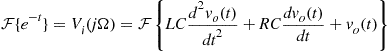 (2.125)
and we get the following result
![]() (2.126)
(2.126)
where the output in the frequency-domain, ![]() , is given by
, is given by
![]() (2.127)
(2.127)
which exhibits a resonant behavior exactly as in (2.96). Also note that the frequency response, defined in (2.93), corresponds to the Fourier transform of the impulse response.
Fourier methods and applications are presented in [1,4,5,16,17].
1.02.8 Conclusion and future trends
This chapter provided an introductory overview on the general concepts of signals, systems, and analysis tools used in the continuous-time domain.
We believe that the knowledge of continuous-time signals and systems, even for a book directed for methods used in the discrete-time domain, is extremely important for, while exploring their differences, the reader can enhance the understanding of the natural phenomena.
A few papers discuss the relevance of teaching (analog) circuits and systems, as well its importance to an engineering career [18].
Analog circuit engineers have to deal with the entire circuit, and many parameters must be considered in their design. In order to simplify circuit models, designers have to make approximations about the analog components, which requires expertise and years of education.
This chapter dealt with traditional electrical components and their fundamental variables: resistors having a direct relationship between voltage and current (![]() the resistance), inductors relating voltage and current with its flux (
the resistance), inductors relating voltage and current with its flux (![]() and
and ![]() the inductance), and capacitors relating voltage and current with charge (
the inductance), and capacitors relating voltage and current with charge (![]() and
and ![]() the capacitance). After first theorized in the early seventies, the memristor regained the media in 2008 when a first real implementation was announced: the fourth fundamental circuit element relating charge and flux as in its axiomatic definition,
the capacitance). After first theorized in the early seventies, the memristor regained the media in 2008 when a first real implementation was announced: the fourth fundamental circuit element relating charge and flux as in its axiomatic definition, ![]() (M the memristance) [19]. The use of this component in usual electronic gadgets as well as teaching its theory even in undergraduate courses seems to be an upcoming technology trend.
(M the memristance) [19]. The use of this component in usual electronic gadgets as well as teaching its theory even in undergraduate courses seems to be an upcoming technology trend.
In addition, most electronic devices have to interface with the external, analog, world, where data conversion is needed at the input and output sides. Analog technologies are used along with digital technologies, spanning from human interface components to analog circuits in wireless components. Furthermore, analog design is also present in the mixed-signal integrated circuits, and it is becoming increasingly critical due to high-speed circuitry [20]. Analog circuits are also used to process signals in very high frequency ranges, such as microwave and RF. In addition, electronic digital circuits are supplied with power, and the trend is to reduce power consumption of digital circuitry. Hence, knowledge of analog circuits is required if an engineer is designing a high performance digital circuit.
We have tried to condense in few pages, all pertinent information regarding analog signals and systems in order to help a complete understanding of the forthcoming chapters. Nevertheless, we have not exhausted the description of all details. For more interested readers, we outline in the following suggested references for further reading. We hope you enjoy the rest of the book.
Glossary
BIBO refers to a certain class of stability known as bounded-input bounded-output
Convolution operation between two functions: the output (zero-state solution) of a linear and time-invariant system corresponds to the convolution integral between the input signal and the impulse response, i.e., ![]()
Frequency response of a linear system corresponds to the Fourier transform of its impulse response: ![]()
Impulse signal ![]() is a pulse of infinite amplitude and infinitesimal time characterized by being equal to zero when
is a pulse of infinite amplitude and infinitesimal time characterized by being equal to zero when ![]() and
and ![]()
Impulse response ![]() is the output of a linear and time-invariant system when the input corresponds to the impulse
is the output of a linear and time-invariant system when the input corresponds to the impulse ![]()
LTI linear and time-invariant system: when the output of a continuous-time system corresponds to a linear operation on the input signal while not depending on a particular instant but remaining the same as time goes by
ODE ordinary differential equation: a differential equation having only one independent variable
RLC is usually related to a circuit with resistor (R), inductor (L) and capacitor (C)
ROC region of convergence of the Laplace transform of a given signal ![]() : in the Laplace transform domain, it corresponds to the set of values of the complex variable s that ensures the existence of
: in the Laplace transform domain, it corresponds to the set of values of the complex variable s that ensures the existence of ![]()
Transfer function is the representation in the s-domain of the input-output relation for a linear system; it corresponds to the Laplace transform of the impulse response, i.e., ![]()
Unit-step signal ![]() is equal to 0 when
is equal to 0 when ![]() , equal to 1 when
, equal to 1 when ![]() and relates to the impulse signal as follows:
and relates to the impulse signal as follows: ![]()
1.02.9 Relevant Websites:
<http://www.britannica.com/EBchecked/topic/330320/Pierre-Simon-marquis-de-Laplace/> (article from the Encyclopedia Britannica about Laplace)
<http://www.genealogy.ams.org/id.php?id=108295> (American Mathematical Society Genealogy Project, Pierre-Simon Laplace)
<http://www.academie-francaise.fr/immortels/base/academiciens/fiche.asp?param=336> (mention to Pierre-Simon de Laplace, immortal of Académie-Française)
<http://www.britannica.com/EBchecked/topic/215097/Joseph-Baron-Fourier/> (article from the Encyclopedia Britannica about Fourier)
<http://www.genealogy.ams.org/id.php?id=17981> (American Mathematical Society Genealogy Project, Jean-Baptiste Joseph Fourier)
<http://www.ieeeghn.org/> (IEEE Global History Network)
<http://www.coe.ufrj.br/∼acmq/> (this site contains many tools for circuit analysis and design as well as a number of interesting links)
Relevant Theory: Signal Processing Theory
1.02.10 Supplementary data
Supplementary data associated with this article can be found, in the online version, at http://dx.doi.org/10.1016/B978-0-12-396502-8.00002-4.

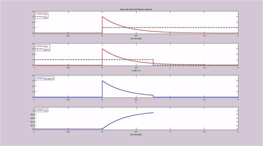

References
1. Oppenheim A, Willsky A, Nawab S. Signals and Systems, Prentice-Hall Signal Processing Series. second ed. Prentice Hall 1996.
2. Lathi BP. Linear Systems and Signals. second ed. Oxford University Press 2004.
3. Lathi BP. Signal Processing and Linear Systems. second ed. Oxford University Press 2009; Incorporated.
4. Haykin S, Veen B. Signals and Systems. second ed. John Wiley & Sons 2003.
5. Girod B, Rabenstein R, Stenger A. Signals and Systems. first ed. John Wiley & Sons 2001.
6. Boyce W, DiPrima R. Elementary differential equations. ninth ed. USA: John Wiley & Sons; 2008.
7. Fischer-Cripps AC. The Mathematics Companion: Mathematical Methods for Physicists and Engineers. New York, USA: Taylor & Francis; 2005.
8. Dorf R, Svoboda J. Introduction to Electric Circuits. eighth ed. USA: John Wiley & Sons; 2010.
9. Strang G. Computational Science and Engineering. Massachusetts, USA: Wellesley-Cambridge Press; 2007.
10. Thomson W. Laplace Transformation, Prentice-Hall Electrical Engineering Series. second ed. Prentice-Hall Inc. 1960.
11. Holbrook J. Laplace transforms for electronic engineers, International Series of Monographs on Electronics and Instrumentation. second ed. Pergamon Press 1966.
12. Oberhettinger F, Badii L. Tables of Laplace transforms, Grundlehren der mathematischen wissenschaften. Springer-Verlag 1973.
13. Padulo L, Arbib MA. System Theory: A Unified State-Space Approach to Continuous and Discrete Systems. Philadelphia, USA: W.B. Saunders Company; 1974.
14. Close C. Analysis of Linear Circuits. California, USA: Harcourt Publishers Ltd.; 1974; International edition.
15. C. Desoer, E. Kuh, Basic circuit theory, McGraw Hill International Editions: Electrical and Electronic Engineering Series, New York, USA, 1969.
16. Bracewell R. The Fourier transform and its applications, McGraw-Hill Series in Electrical and Computer Engineering. third ed. McGraw Hill 2000.
17. Papoulis A. The Fourier integral and its applications, McGraw-Hill Electronic Sciences Series. McGraw-Hill 1962.
18. P. Diniz, Teaching circuits, systems, and signal processing, in: Proceedings of the 1998 IEEE International Symposium on Circuits and Systems 1998, ISCAS’98, vol. 1, 1998, pp. 428–431, <http://dx.doi.org/10.1109/ISCAS.1998.704468>.
19. Pazienza GE, Albo-Canals J. Teaching memristors to EE undergraduate students [class notes]. IEEE Circ Syst Mag. 2011;11(4):36–44.
20. R. Gray, History and trends in analog circuit challenges at the system level, in: 2010 International Symposium on Electronic System Design (ISED), 2010, p. 24, doi: <http://dx.doi.org/10.1109/ISED.2010.62>.
1Authors thank Prof. Ney Bruno for his kind and competent review of this chapter.