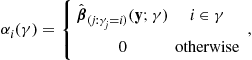
A Tutorial on Model Selection
Enes Makalic*, Daniel Francis Schmidt* and Abd-Krim Seghouane†, *Centre for M.E.G.A. Epidemiology, The University of Melbourne, Australia, †Department of Electrical and Electronic Engineering, The University of Melbourne, Australia
Abstract
Model selection is a key problem in many areas of science and engineering. Given a data set, model selection involves finding the statistical model that best captures the properties and regularities present in the data. This chapter examines three broad approaches to model selection: (i) minimum distance estimation criteria, (ii) Bayesian statistics, and (iii) model selection by data compression. Model selection in the context of linear regression is used as a running example throughout the chapter
Keywords
Model selection; Maximum likelihood; Akaike information criterion (AIC); Bayesian information criterion (BIC); Minimum message length (MML); Minimum description length (MDL)
1.25.1 Introduction
A common and widespread problem in science and engineering is the determination of a suitable model to describe or characterize an experimental data set. This determination consists of two tasks: (i) the choice of an appropriate model structure, and (ii) the estimation of the associated model parameters. Given the structure or dimension of the model, the task of parameter estimation is generally done by maximum likelihood or least squares procedures. The choice of the dimension of a model is often facilitated by the use of a model selection criterion. The key idea underlying most model selection criteria is the parsimonity principle which says that there should be a tradeoff between data fit and complexity. This chapter examines three broad approaches to model selection commonly applied in the literature: (i) methods that attempt to estimate the distance between the fitted model and the unknown distribution that generated the data (see Section 1.25.2); (ii) Bayesian approaches which use the posterior distribution of the parameters to make probabilistic statements about the plausibility of the fitted models (see Section 1.25.3), and (iii) information theoretic model selection procedures that measure the quality of the fitted models by how well these models compress the data (see Section 1.25.4).
Formally, we observe a sample of n data points ![]() from an unknown probability distribution
from an unknown probability distribution ![]() . The model selection problem is to learn a good approximation to
. The model selection problem is to learn a good approximation to ![]() using only the observed data
using only the observed data ![]() . This problem is intractable unless some assumptions are made about the unknown distribution
. This problem is intractable unless some assumptions are made about the unknown distribution ![]() . The assumption made in this chapter is that
. The assumption made in this chapter is that ![]() can be adequately approximated by one of the distributions from a set of parametric models
can be adequately approximated by one of the distributions from a set of parametric models ![]() where
where ![]() defines the model structure and the parameter vector
defines the model structure and the parameter vector ![]() indexes a particular distribution from the model
indexes a particular distribution from the model ![]() . The dimensionality of
. The dimensionality of ![]() will always be clear from the context. As an example, if we are interested in inferring the order of a polynomial in a linear regression problem, the set
will always be clear from the context. As an example, if we are interested in inferring the order of a polynomial in a linear regression problem, the set ![]() may include first-order, second-order and third-order polynomials. The parameter vector
may include first-order, second-order and third-order polynomials. The parameter vector ![]() then represents the coefficients for a particular polynomial; for example, the intercept and linear term for the first-order model. The model selection problem is to infer an appropriate model structure
then represents the coefficients for a particular polynomial; for example, the intercept and linear term for the first-order model. The model selection problem is to infer an appropriate model structure ![]() and parameter vector
and parameter vector ![]() that provide a good approximation to the data generating distribution
that provide a good approximation to the data generating distribution ![]() .
.
This chapter largely focuses on the inference of the model structure ![]() . A common approach to estimating the parameters
. A common approach to estimating the parameters ![]() for a given model
for a given model ![]() is the method of maximum likelihood. Here, the parameter vector is chosen such that the probability of the observed data
is the method of maximum likelihood. Here, the parameter vector is chosen such that the probability of the observed data ![]() is maximized, that is
is maximized, that is
![]() (25.1)
(25.1)
where ![]() denotes the likelihood of the data under the distribution indexed by
denotes the likelihood of the data under the distribution indexed by ![]() . This is a powerful approach to parameter estimation that possesses many attractive statistical properties [1]. However, it is not without its flaws, and as part of this chapter we will examine an alternative method of parameter estimation that should sometimes be preferred to maximum likelihood (see Section 1.25.4.2). The statistical theory underlying model selection is often abstract and difficult to understand in isolation, and it is helpful to consider these concepts within the context of a practical example. To this end, we have chosen to illustrate the application of the model selection criteria discussed in this chapter to the important and commonly used linear regression model.
. This is a powerful approach to parameter estimation that possesses many attractive statistical properties [1]. However, it is not without its flaws, and as part of this chapter we will examine an alternative method of parameter estimation that should sometimes be preferred to maximum likelihood (see Section 1.25.4.2). The statistical theory underlying model selection is often abstract and difficult to understand in isolation, and it is helpful to consider these concepts within the context of a practical example. To this end, we have chosen to illustrate the application of the model selection criteria discussed in this chapter to the important and commonly used linear regression model.
1.25.1.1 Nested and non-nested sets of candidate models
The structure of the set of candidate models ![]() can have a significant effect on the performance of model selection criteria. There are two general types of candidate model sets: nested sets of candidate models, and non-nested sets of candidate models. Nested sets of candidate models have special properties that make model selection easier and this structure is often assumed in the derivation of model selection criteria, such as in the case of the distance based methods of Section 1.25.2. Let us partition the model set
can have a significant effect on the performance of model selection criteria. There are two general types of candidate model sets: nested sets of candidate models, and non-nested sets of candidate models. Nested sets of candidate models have special properties that make model selection easier and this structure is often assumed in the derivation of model selection criteria, such as in the case of the distance based methods of Section 1.25.2. Let us partition the model set ![]() , where the subsets
, where the subsets ![]() are the set of all candidate models with k free parameters. A candidate set
are the set of all candidate models with k free parameters. A candidate set ![]() is considered nested if: (1) there is only one candidate model with k parameters (
is considered nested if: (1) there is only one candidate model with k parameters (![]() for all k), and (2) models
for all k), and (2) models ![]() with k parameters can exactly represent all distributions indexed by models with less than k parameters. That is, if
with k parameters can exactly represent all distributions indexed by models with less than k parameters. That is, if ![]() is a model with k free parameters, and model
is a model with k free parameters, and model ![]() is a model with l free parameters, where
is a model with l free parameters, where ![]() , then
, then
![]()
A canonical example of a nested model structure is the polynomial order selection problem. Here, a second-order model can exactly represent any first-order model by setting the quadratic term to zero. Similarly, a third-order model can exactly represent any first-order or second-order model by setting the appropriate parameters to zero, and so on. In the non-nested case, there is not necessarily only a single model with k parameters, and there is no requirement that models with more free parameters can exactly represent all simpler models. This can introduce difficulties for some model selection criteria, and it is thus important to be aware of the structure of the set ![]() before choosing a particular criterion to apply. The concept of nested and non-nested model sets will be made clearer in the following linear regression example.
before choosing a particular criterion to apply. The concept of nested and non-nested model sets will be made clearer in the following linear regression example.
1.25.1.2 Example: the linear model
Linear regression is of great importance in engineering and signal processing as it appears in a wide range of problems such as smoothing a signal with polynomials, estimating the number of sinusoids in noisy data and modeling linear dynamic systems. The linear regression model for explaining data ![]() assumes that the means of the observations are a linear combination of
assumes that the means of the observations are a linear combination of ![]() measured variables, or covariates, that is,
measured variables, or covariates, that is,
![]() (25.2)
(25.2)
where ![]() is the full design matrix,
is the full design matrix, ![]() are the parameter coefficients and
are the parameter coefficients and ![]() are independent and identically distributed Gaussian variates
are independent and identically distributed Gaussian variates ![]() . Model selection in the linear regression context arises because it is common to assume that only a subset of the covariates is associated with the observations; that is, only a subset of the parameter vector is non-zero. Let
. Model selection in the linear regression context arises because it is common to assume that only a subset of the covariates is associated with the observations; that is, only a subset of the parameter vector is non-zero. Let ![]() denote an index set determining which of the covariates comprise the design submatrix
denote an index set determining which of the covariates comprise the design submatrix ![]() ; the set of all candidate subsets is denoted by
; the set of all candidate subsets is denoted by ![]() . The linear model indexed by
. The linear model indexed by ![]() is then
is then
![]() (25.3)
(25.3)
where ![]() is the parameter vector of size
is the parameter vector of size ![]() and
and
![]()
The total number of unknown parameters to be estimated for model ![]() , including the noise variance parameter, is
, including the noise variance parameter, is ![]() . The negative log-likelihood for the data
. The negative log-likelihood for the data ![]() is
is
![]() (25.4)
(25.4)
The maximum likelihood estimates for the coefficient ![]() and the noise variance
and the noise variance ![]() are
are
![]() (25.5)
(25.5)
![]() (25.6)
(25.6)
which coincide with the estimates obtained by minimising the sum of squared errors (the least squares estimates). The negative log-likelihood evaluated at the maximum likelihood estimates is given by
![]() (25.7)
(25.7)
The structure of the set ![]() in the context of the linear regression model depends on the nature and interpretation of the covariates. In the case that the covariates are polynomials of increasing order, or sinusoids of increasing frequency, it is often convenient to assume a nested structure on
in the context of the linear regression model depends on the nature and interpretation of the covariates. In the case that the covariates are polynomials of increasing order, or sinusoids of increasing frequency, it is often convenient to assume a nested structure on ![]() . For example, let us assume that the
. For example, let us assume that the ![]() covariates are polynomials such that
covariates are polynomials such that ![]() is the zero-order term (constant),
is the zero-order term (constant), ![]() the linear term,
the linear term, ![]() the quadratic term and
the quadratic term and ![]() the cubic term. To use a model selection criterion to select an appropriate order of polynomial, we can form the set of candidate models
the cubic term. To use a model selection criterion to select an appropriate order of polynomial, we can form the set of candidate models ![]() as
as
![]()
where
![]()
From this structure it is obvious that there is only one model with k free parameters, for all k, and that models with more parameters can exactly represent all models with less parameters by setting the appropriate coefficients to zero. In contrast, consider the situation in which the covariates have no natural ordering, or that we do not wish to impose an ordering; for example, in the case of polynomial regression, we may wish to determine which, if any, of the individual polynomial terms are associated with the observations. In this case there is no clear way of imposing a nested structure, as we cannot a priori rule out any particular combination of covariates being important. This is usually called the all-subsets regression problem, and the candidate model set then has the following structure
where ![]() denotes the empty set, that is, none of the covariates are to be used. It is clear that models with more parameters can not necessarily represent all models with less parameters; for example, the model
denotes the empty set, that is, none of the covariates are to be used. It is clear that models with more parameters can not necessarily represent all models with less parameters; for example, the model ![]() cannot represent the model
cannot represent the model ![]() as it is lacking covariate
as it is lacking covariate ![]() . Further, there is now no longer just a single model with k free parameters; in the above example, there are four models with one free parameter, and six models with two free parameters. In general, if there are q covariates in total, the number of models with k free parameters is given by
. Further, there is now no longer just a single model with k free parameters; in the above example, there are four models with one free parameter, and six models with two free parameters. In general, if there are q covariates in total, the number of models with k free parameters is given by ![]() , which may be substantially greater than one for moderate q.
, which may be substantially greater than one for moderate q.
Throughout the remainder of this chapter, the linear model example will be used to demonstrate the practical application of the model selection criteria that will be discussed.
1.25.2 Minimum distance estimation criteria
Intuitively, model selection criteria can be derived by quantifying “how close” the probability density of the fitted model is to the unknown, generating distribution. Many measures of distance between two probability distributions exist in the literature. Due to several theoretical properties, the Kullback-Leibler divergence [2], and its variants, is perhaps the most frequently used information theoretic measure of distance.
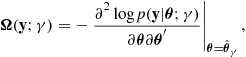
As the distribution ![]() that generated the observations
that generated the observations ![]() is unknown, the basic idea underlying the minimum distance estimation criteria is to construct an estimate of how close the fitted distributions are to the truth. In general, these estimators are constructed to satisfy the property of unbiasedness, at least for large sample sizes n. In particular, the distance-based methods we examine are the well known Akaike information criterion (AIC) (see Section 1.25.2.1) and symmetric Kullback information criterion (KIC) (see Section 1.25.2.2), as well as several corrected variants that improve the performance of these criteria when the sample size is small.
is unknown, the basic idea underlying the minimum distance estimation criteria is to construct an estimate of how close the fitted distributions are to the truth. In general, these estimators are constructed to satisfy the property of unbiasedness, at least for large sample sizes n. In particular, the distance-based methods we examine are the well known Akaike information criterion (AIC) (see Section 1.25.2.1) and symmetric Kullback information criterion (KIC) (see Section 1.25.2.2), as well as several corrected variants that improve the performance of these criteria when the sample size is small.
1.25.2.1 The Akaike information criterion
Recall the model selection problem as introduced in Section 1.25.1. Suppose a collection of n observations ![]() has been sampled from an unknown distribution
has been sampled from an unknown distribution ![]() having density function
having density function ![]() . Estimation of
. Estimation of ![]() is done within a set of nested candidate models
is done within a set of nested candidate models ![]() , characterized by probability densities
, characterized by probability densities ![]() , where
, where ![]() and
and ![]() is the number of free parameters possessed by model
is the number of free parameters possessed by model ![]() . Let
. Let ![]() denote the vector of estimated parameters obtained by maximizing the likelihood
denote the vector of estimated parameters obtained by maximizing the likelihood ![]() over
over ![]() , that is,
, that is,
![]()
and let ![]() denote the corresponding fitted model. To simplify notation, we introduce the shorthand notation
denote the corresponding fitted model. To simplify notation, we introduce the shorthand notation ![]() to denote the maximum likelihood estimator, and
to denote the maximum likelihood estimator, and ![]() to denote the maximized likelihood for model
to denote the maximized likelihood for model ![]() .
.
To determine which candidate density model best approximates the true unknown model ![]() , we require a measure which provides a suitable reflection of the separation between
, we require a measure which provides a suitable reflection of the separation between ![]() and an approximating model
and an approximating model ![]() . The Kullback-Leibler divergence, also known as the cross-entropy, is one such measure. For the two probability densities
. The Kullback-Leibler divergence, also known as the cross-entropy, is one such measure. For the two probability densities ![]() and
and ![]() , the Kullback-Leibler divergence,
, the Kullback-Leibler divergence, ![]() , between
, between ![]() and
and ![]() with respect to
with respect to ![]() is defined as
is defined as
where
![]() (25.8)
(25.8)
and ![]() represents the expectation with respect to
represents the expectation with respect to ![]() , that is,
, that is, ![]() . Ideally, the selection of the best model from the set of candidate models
. Ideally, the selection of the best model from the set of candidate models ![]() would be done by choosing the model with the minimum KL divergence from the data generating distribution
would be done by choosing the model with the minimum KL divergence from the data generating distribution ![]() , that is
, that is
![]()
where ![]() is the maximum likelihood estimator of the parameters of model
is the maximum likelihood estimator of the parameters of model ![]() based on the observed data
based on the observed data ![]() . Since
. Since ![]() does not depend on the fitted model
does not depend on the fitted model ![]() , any ranking of the candidate models according to
, any ranking of the candidate models according to ![]() is equivalent to ranking the models according to
is equivalent to ranking the models according to ![]() . Unfortunately, evaluating
. Unfortunately, evaluating ![]() is not possible since doing so requires the knowledge of
is not possible since doing so requires the knowledge of ![]() which is the aim of model selection in the first place.
which is the aim of model selection in the first place.
As noted by Takeuchi [3], twice the negative maximized log-likelihood, ![]() , acts as a downwardly biased estimator of
, acts as a downwardly biased estimator of ![]() and is therefore not suitable for model comparison by itself. An unbiased estimate of the KL divergence is clearly of interest and could be used as a tool for model selection. It can be shown that the bias in estimation is given by
and is therefore not suitable for model comparison by itself. An unbiased estimate of the KL divergence is clearly of interest and could be used as a tool for model selection. It can be shown that the bias in estimation is given by
![]() (25.9)
(25.9)
which, under suitable regularity conditions can be asymptotically estimated by [4,5]
![]() (25.10)
(25.10)
where
 (25.11)
![]() (25.12)
(25.12)
and ![]() denotes the trace of a matrix. The parameter vector
denotes the trace of a matrix. The parameter vector ![]() defined by
defined by
![]() (25.13)
(25.13)
indexes the distribution in the model ![]() that is closest to the data generating distribution
that is closest to the data generating distribution ![]() in terms of KL divergence. Unfortunately, the parameter vector
in terms of KL divergence. Unfortunately, the parameter vector ![]() is unknown and so one cannot compute the required bias adjustment. However, Takeuchi [3] noted that under suitable regularity conditions, the maximum likelihood estimate can be used in place of
is unknown and so one cannot compute the required bias adjustment. However, Takeuchi [3] noted that under suitable regularity conditions, the maximum likelihood estimate can be used in place of ![]() to derive an approximation to (25.10), leading to the Takeuchi Information Criterion (TIC)
to derive an approximation to (25.10), leading to the Takeuchi Information Criterion (TIC)
![]() (25.14)
(25.14)
where
 (25.15)
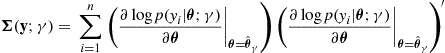 (25.16)
are empirical estimates of the matrices (25.11) and (25.12), respectively. To use the TIC for model selection, we choose the model ![]() with the smallest TIC score, that is
with the smallest TIC score, that is
![]()
The model with the smallest TIC score corresponds to the model we believe to be the closest in terms of KL divergence to the data generating distribution ![]() . Under suitable regularity conditions, the TIC is an unbiased estimate of the KL divergence between the fitted model
. Under suitable regularity conditions, the TIC is an unbiased estimate of the KL divergence between the fitted model ![]() and the data generating model
and the data generating model ![]() , that is
, that is
![]()
where ![]() is a quantity that vanishes as
is a quantity that vanishes as ![]() . The empirical matrices (25.15) and (25.16) are a good approximation to (25.11) and (25.12) only if the sample size n is very large. As this is often not the case in practice, the TIC is rarely used.
. The empirical matrices (25.15) and (25.16) are a good approximation to (25.11) and (25.12) only if the sample size n is very large. As this is often not the case in practice, the TIC is rarely used.
The dependence of the TIC on the empirical matrices can be avoided if one assumes that the data generating distribution ![]() is a distribution contained in the model
is a distribution contained in the model ![]() . In this case, the matrices (25.11) and (25.12) coincide. Thus,
. In this case, the matrices (25.11) and (25.12) coincide. Thus, ![]() reduces to the number of parameters k, and we obtain the widely known and extensively used Akaike’s Information Criterion (AIC) [6]
reduces to the number of parameters k, and we obtain the widely known and extensively used Akaike’s Information Criterion (AIC) [6]
![]() (25.17)
(25.17)
An interesting way to view the AIC (25.17) is as a penalized likelihood criterion. For a given model ![]() , the negative maximized log-likelihood measures how well the model fits the data, while the “
, the negative maximized log-likelihood measures how well the model fits the data, while the “![]() ” penalty measures the complexity of the model. Clearly, the complexity is an increasing function of the number of free parameters, and this acts to naturally balance the complexity of a model against its fit. Practically, this means that a complex model must fit the data well to be preferred to a simpler model with a similar quality of fit.
” penalty measures the complexity of the model. Clearly, the complexity is an increasing function of the number of free parameters, and this acts to naturally balance the complexity of a model against its fit. Practically, this means that a complex model must fit the data well to be preferred to a simpler model with a similar quality of fit.
Similar to the TIC, the AIC is an asymptotically unbiased estimator of the KL divergence between the generating distribution ![]() and the fitted distribution
and the fitted distribution ![]() , that is
, that is
![]()
When the sample size is large and the number of free parameters is small relative to the sample size, the ![]() term is approximately zero, and the AIC offers an excellent estimate of the Kullback-Leibler divergence. However, in the case that n is small, or k is large relative to n, the
term is approximately zero, and the AIC offers an excellent estimate of the Kullback-Leibler divergence. However, in the case that n is small, or k is large relative to n, the ![]() term may be quite large, and the AIC does not adequately correct the bias, making it unsuitable for model selection.
term may be quite large, and the AIC does not adequately correct the bias, making it unsuitable for model selection.
To address this issue, Hurvich and Tsai [7] proposed a small sample correction to the AIC in the linear regression setting. This small sample AIC, referred to as AICc, is given by
![]() (25.18)
(25.18)
for a model ![]() with k free parameters, and has subsequently been applied to models other than linear regressions. From (25.18) it is clear that the penalty term is substantially larger than
with k free parameters, and has subsequently been applied to models other than linear regressions. From (25.18) it is clear that the penalty term is substantially larger than ![]() when the sample size n is not significantly larger than k, and that as
when the sample size n is not significantly larger than k, and that as ![]() the AICc is equivalent to the regular AIC (25.17). Practically, a large body of empirical evidence strongly suggests that the AICc performs significantly better as a model selection tool than the AIC, largely irrespective of the problem. The approach taken by Hurvich and Tsai to derive their AICc criterion is not the only way of deriving small sample minimum distance estimators based on the KL divergence; for example, the work in [8] derives alternative AIC-like criteria based on variants of the KL divergence, while [9] offers an alternative small sample criterion obtained through bootstrap approximations.
the AICc is equivalent to the regular AIC (25.17). Practically, a large body of empirical evidence strongly suggests that the AICc performs significantly better as a model selection tool than the AIC, largely irrespective of the problem. The approach taken by Hurvich and Tsai to derive their AICc criterion is not the only way of deriving small sample minimum distance estimators based on the KL divergence; for example, the work in [8] derives alternative AIC-like criteria based on variants of the KL divergence, while [9] offers an alternative small sample criterion obtained through bootstrap approximations.
For the reader interested in the theoretical details and complete derivations of the AIC, including all regularity conditions, we highly recommend the excellent text by Linhart and Zucchini [5]. We also recommend the text by McQuarrie and Tsai [10] for a more practical treatment of AIC and AICc.
1.25.2.2 The Kullback information criterion
Since the Kullback-Leibler divergence is an asymmetric measure, an alternative directed divergence can be obtained by reversing the roles of the two models in the definition of the measure. A undirected measure of model dissimilarity can be obtained from the sum of the two directed divergences. This measure is known as Kullback’s symmetric divergence, or J-divergence [11]. Since the J-divergence combines information about model dissimilarity through two distinct measures, it functions as a gauge of model disparity which is arguably more sensitive than either of its individual components. The J-divergence, ![]() , between the true generating distribution
, between the true generating distribution ![]() and a distribution
and a distribution ![]() is given by
is given by
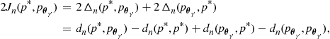
where
![]() (25.19)
(25.19)
![]() (25.20)
(25.20)
As in Section (1.25.2.1), we note that the term ![]() does not depend on the fitted model
does not depend on the fitted model ![]() and may be dropped when ranking models. The quantity
and may be dropped when ranking models. The quantity
![]()
may then be used as a surrogate for the J-divergence, and leads to an appealing measure of dissimilarity between the generating distribution and the fitted candidate model. In a similar fashion to the AIC, twice the negative maximized log-likelihood has been shown to be a downwardly biased estimate of the J-divergence. Cavanaugh [12] derives an estimate of this bias, and uses this correction to define a model selection criterion called KIC (symmetric Kullback information criterion), which is given by
![]() (25.21)
(25.21)
Comparing (25.21) to the AIC (25.17), we see that the KIC complexity penalty is slightly greater. This implies that the KIC tends to prefer simpler models (that is, those with less parameters) than those selected by minimising the AIC. Under suitable regularity conditions, the KIC satisfies
![]()
Empirically, the KIC has been shown to outperform AIC in large sample linear regression and autoregressive model selection, and tends to lead to less overfitting than AIC. Similarly to the AIC, when the sample size n is small the bias correction term ![]() is too small, and the KIC performs poorly as a model selection tool. Seghouane and Bekara [13] derived a corrected KIC, called KICc, in the context of linear regression that is suitable for use when the sample size is small relative to the total number of parameters k. The KICc is
is too small, and the KIC performs poorly as a model selection tool. Seghouane and Bekara [13] derived a corrected KIC, called KICc, in the context of linear regression that is suitable for use when the sample size is small relative to the total number of parameters k. The KICc is
![]() (25.22)
(25.22)
where ![]() denotes the digamma function. The digamma function can be difficult to compute, and approximating the digamma function by a second-order Taylor series expansion yields the so called AKICc, which is given by
denotes the digamma function. The digamma function can be difficult to compute, and approximating the digamma function by a second-order Taylor series expansion yields the so called AKICc, which is given by
![]() (25.23)
(25.23)
The second term in (25.22) appears as the complexity penalty in the AICc(25.18), which is not surprising given that the J-divergence is a sum of two KL divergence functions. Empirically, the KICc has been shown to outperform the KIC as a model selection tool when the sample size is small.
1.25.2.3 Example application: linear regression
We now demonstrate the application of the minimum distance estimation criteria to the problem of linear regression introduced in Section 1.25.1.2. Recall that in this setting, ![]() specifies which covariates from the full design matrix
specifies which covariates from the full design matrix ![]() should be used in the fitted model. The total number of parameters is therefore
should be used in the fitted model. The total number of parameters is therefore ![]() , where the additional parameter accounts for the fact that we must estimate the noise variance. The various model selection criteria are listed below:
, where the additional parameter accounts for the fact that we must estimate the noise variance. The various model selection criteria are listed below:
![]() (25.24)
(25.24)
![]() (25.25)
(25.25)
![]() (25.26)
(25.26)
![]() (25.27)
(25.27)
It is important to stress that all these criteria are derived within the context of a nested set of candidate models ![]() (see Section 1.25.1.1). In the next section we will briefly examine the problems that can arise if these criteria are used in situations where the candidates are not nested.
(see Section 1.25.1.1). In the next section we will briefly examine the problems that can arise if these criteria are used in situations where the candidates are not nested.
1.25.2.4 Consistency and efficiency
Let ![]() denote the model that generated the observed data
denote the model that generated the observed data ![]() and assume that
and assume that ![]() is a member of the set of candidate models
is a member of the set of candidate models ![]() which is fixed and does not grow with sample size n; recall that the model
which is fixed and does not grow with sample size n; recall that the model ![]() contains the data generating distribution
contains the data generating distribution ![]() as a particular distribution. Furthermore, of all the models that contain
as a particular distribution. Furthermore, of all the models that contain ![]() , the model
, the model ![]() has the least number of free parameters. A model selection criterion is consistent if the probability of selecting the true model
has the least number of free parameters. A model selection criterion is consistent if the probability of selecting the true model ![]() approaches one as the sample size
approaches one as the sample size ![]() . None of the distance based criteria examined in this chapter are consistent model selection procedures. This means that even for extremely large sample sizes, there is a non-zero probability that these distance based criteria will overfit and select a model with more free parameters than
. None of the distance based criteria examined in this chapter are consistent model selection procedures. This means that even for extremely large sample sizes, there is a non-zero probability that these distance based criteria will overfit and select a model with more free parameters than ![]() . Consequently, if the aim of the experiment is to discover the true model, the aforementioned distance based criteria are inappropriate. For example, in the linear regression setting, if the primary aim of the model selection exercise is to determine only those covariates that are associated with the observations, one should not use the AIC or KIC (and their variants).
. Consequently, if the aim of the experiment is to discover the true model, the aforementioned distance based criteria are inappropriate. For example, in the linear regression setting, if the primary aim of the model selection exercise is to determine only those covariates that are associated with the observations, one should not use the AIC or KIC (and their variants).
In contrast, if the true model is of infinite order, which in many settings may be deemed more realistic in practice, then the true model lies outside the class of candidate models. In this case, we cannot hope to discover the true model, and instead would like our model selection criterion to at least provide good predictions about future data arising from the same source. A criterion that minimizes the one-step mean squared error between the fitted model and the generating distribution ![]() with high probability as
with high probability as ![]() is termed efficient. The AIC and KIC, and their corrected variants are all asymptotically efficient [4]. This suggests that for large sample sizes, model selection by distance based criteria will lead to adequate prediction errors even if the true model lies outside the set of candidate models
is termed efficient. The AIC and KIC, and their corrected variants are all asymptotically efficient [4]. This suggests that for large sample sizes, model selection by distance based criteria will lead to adequate prediction errors even if the true model lies outside the set of candidate models ![]() .
.
1.25.2.5 The AIC and KIC for non-nested sets of candidate models
The derivations of the AIC and KIC, and their variants, depend on the assumption that the candidate model set ![]() is nested. We conclude this section by briefly examining the behavior of these criteria when they are used to select a model from a non-nested candidate model set. First, consider the case that
is nested. We conclude this section by briefly examining the behavior of these criteria when they are used to select a model from a non-nested candidate model set. First, consider the case that ![]() forms a nested set of models, and let
forms a nested set of models, and let ![]() be the true model, that is, the model that generated the data; this means that
be the true model, that is, the model that generated the data; this means that ![]() is the model in
is the model in ![]() with the least number of free parameters, say
with the least number of free parameters, say ![]() , that contains the data generating distribution
, that contains the data generating distribution ![]() as a particular distribution. If n is sufficiently large, the probability that the model selected by minimising the AIC will have
as a particular distribution. If n is sufficiently large, the probability that the model selected by minimising the AIC will have ![]() parameters is at least 16%, with the equivalent probability for KIC being approximately 8% [10].
parameters is at least 16%, with the equivalent probability for KIC being approximately 8% [10].
Consider now the case in which ![]() forms a non-nested set of candidate models. A recent paper by Schmidt and Makalic [14] has demonstrated that in this case, the AIC is a downwardly biased estimator of the Kullback-Leibler divergence even asymptotically in n, and this downward bias is determined by the size of the sets
forms a non-nested set of candidate models. A recent paper by Schmidt and Makalic [14] has demonstrated that in this case, the AIC is a downwardly biased estimator of the Kullback-Leibler divergence even asymptotically in n, and this downward bias is determined by the size of the sets ![]() . This implies, that in the case of all-subsets regression, the probability of overfitting is an increasing function of the number of covariates under consideration, q, and this probability cannot be reduced even by increasing the sample size.
. This implies, that in the case of all-subsets regression, the probability of overfitting is an increasing function of the number of covariates under consideration, q, and this probability cannot be reduced even by increasing the sample size.
As an example of how great this probability may be, we consider an all-subsets regression in which the generating distribution is the null model; that is, none of the measured covariates ![]() are associated with the observations
are associated with the observations ![]() . Even if there is only as few as
. Even if there is only as few as ![]() covariates available for selection, the probability of erroneously preferring a non-null model to the null model using the AIC is approximately
covariates available for selection, the probability of erroneously preferring a non-null model to the null model using the AIC is approximately ![]() , and by the time
, and by the time ![]() , this probability rises to
, this probability rises to ![]() . Although [14] examines only the AIC, similar arguments follow easily for the KIC. It is therefore recommended that while both criteria are appropriate for nested model selection, neither of these distance based criteria should be used for model selection in a non-nested situation, such as the all-subsets regression problem.
. Although [14] examines only the AIC, similar arguments follow easily for the KIC. It is therefore recommended that while both criteria are appropriate for nested model selection, neither of these distance based criteria should be used for model selection in a non-nested situation, such as the all-subsets regression problem.
1.25.2.6 Applications
Minimum distance estimation criteria have been widely applied in the literature, and we present below an inexhaustive list of successful applications:
• univariate linear regression models [7,13],
• multivariate linear regression models with arbitrary noise covariance matrices [15,16],
• autoregressive model selection [7,12,17],
• selection of smoothing parameters in nonparametric regression [18],
• selection of the size of a multilayer perceptron network [21].
• model selection in the presence of missing data [22].
For details of many of these applications the reader is referred to [10].
1.25.3 Bayesian approaches to model selection
Section 1.25.2 has described model selection criteria that are designed to explicitly minimise the distance between the estimated models and the true model that generated the observed data ![]() . An alternative approach, based on Bayesian statistics [23], is now discussed. The Bayesian approach to statistical analysis differs from the “classical” approach through the introduction of a prior distribution that is used to quantify an experimenter’s a priori (that is, before the observation of data) beliefs about the source of the observed data. A central quantity in Bayesian analysis is the so-called posterior distribution; given a prior distribution,
. An alternative approach, based on Bayesian statistics [23], is now discussed. The Bayesian approach to statistical analysis differs from the “classical” approach through the introduction of a prior distribution that is used to quantify an experimenter’s a priori (that is, before the observation of data) beliefs about the source of the observed data. A central quantity in Bayesian analysis is the so-called posterior distribution; given a prior distribution, ![]() , over the parameter space
, over the parameter space ![]() , and the likelihood function,
, and the likelihood function, ![]() , the posterior distribution of the parameters given the data may be found by applying Bayes’ theorem, yielding
, the posterior distribution of the parameters given the data may be found by applying Bayes’ theorem, yielding
![]() (25.28)
(25.28)
where
![]() (25.29)
(25.29)
is known as the marginal probability of ![]() for model
for model ![]() , and is a normalization term required to render (25.28) a proper distribution. In general, the specification of the prior distribution may itself depend on further parameters, usually called hyperparameters, but for the purposes of the present discussion this possibility will not be considered. The main strength of the Bayesian paradigm is that it allows uncertainty about models and parameters to be defined directly in terms of probabilities; there is no need to appeal to more abstruse concepts, such as the “confidence interval” of classical statistics. However, there is in general no free lunch in statistics, and this strength comes at a price: the specification and origin of the prior distribution. There are essentially two main schools of thought on this topic: (i) subjective Bayesianism, where prior distributions are viewed as serious expressions of subjective belief about the process that generated the data, and (ii) objective Bayesianism [24], where one attempts to express prior ignorance through the use of uninformative, objective distributions, such as the Jeffreys’ prior [11], reference priors [25] and intrinsic priors [26]. The specification of the prior distribution is the basis of most criticism leveled at the Bayesian school, and an extensive discussion on the merits and drawbacks of Bayesian procedures, and the relative merits of subjective and objective approaches, is beyond the scope of this tutorial (there are many interesting discussions on this topic in the literature, see for example, [27,28]). However, in this section of the tutorial, an approach to the problem of prior distribution specification based on asymptotic arguments will be presented.
, and is a normalization term required to render (25.28) a proper distribution. In general, the specification of the prior distribution may itself depend on further parameters, usually called hyperparameters, but for the purposes of the present discussion this possibility will not be considered. The main strength of the Bayesian paradigm is that it allows uncertainty about models and parameters to be defined directly in terms of probabilities; there is no need to appeal to more abstruse concepts, such as the “confidence interval” of classical statistics. However, there is in general no free lunch in statistics, and this strength comes at a price: the specification and origin of the prior distribution. There are essentially two main schools of thought on this topic: (i) subjective Bayesianism, where prior distributions are viewed as serious expressions of subjective belief about the process that generated the data, and (ii) objective Bayesianism [24], where one attempts to express prior ignorance through the use of uninformative, objective distributions, such as the Jeffreys’ prior [11], reference priors [25] and intrinsic priors [26]. The specification of the prior distribution is the basis of most criticism leveled at the Bayesian school, and an extensive discussion on the merits and drawbacks of Bayesian procedures, and the relative merits of subjective and objective approaches, is beyond the scope of this tutorial (there are many interesting discussions on this topic in the literature, see for example, [27,28]). However, in this section of the tutorial, an approach to the problem of prior distribution specification based on asymptotic arguments will be presented.
While (25.28) specifies a probability distribution over the parameter space ![]() , conditional on the observed data, it gives no indication of the likelihood of the model
, conditional on the observed data, it gives no indication of the likelihood of the model ![]() given the observed data. A common approach is based on the marginal distribution (25.29). If a further prior distribution,
given the observed data. A common approach is based on the marginal distribution (25.29). If a further prior distribution, ![]() , over the set of candidate models
, over the set of candidate models ![]() is available, one may apply Bayes’ theorem to form a posterior distribution over the models themselves, given by
is available, one may apply Bayes’ theorem to form a posterior distribution over the models themselves, given by
![]() (25.30)
(25.30)
Model selection then proceeds by choosing the model ![]() that maximizes the probability (25.30), that is
that maximizes the probability (25.30), that is
![]() (25.31)
(25.31)
where the normalizing constant may be safely ignored. An interesting consequence of the posterior distribution (25.30) is that the posterior-odds in favor of some model, ![]() , over another model
, over another model ![]() , usually called the Bayes factor [29,30], can be found from the ratio of posterior probabilities, that is,
, usually called the Bayes factor [29,30], can be found from the ratio of posterior probabilities, that is,
![]() (25.32)
(25.32)
This allows for a straightforward and highly interpretable quantification of the uncertainty in the choice of any particular model. The most obvious weakness in the Bayesian approach, ignoring the origin of the prior distributions, is computational. As a general rule, the integral in the definition of the marginal distribution (25.29), does not admit a closed-form solution and one must resort to numerical approaches or approximations. The next section will discuss a criterion based on asymptotic arguments that circumvents both the requirement to specify an appropriate prior distribution as well as the issue of integration in the computation of the marginal distribution.
1.25.3.1 The Bayesian information criterion (BIC)
The Bayesian Information Criterion (BIC), also sometimes known as the Schwarz Information Criterion (SIC), was proposed by Schwarz [31]. However, the resulting criterion is not unique and was also derived from information theoretic considerations by Rissanen [32], as well as being implicit in the earlier work of Wallace and Boulton [33]; the information theoretic arguments for model selection are discussed in detail in the next section of this chapter. The BIC is based on the Laplace approximation for high dimensional integration [34]. Essentially, under certain regularity conditions, the Laplace approximation works by replacing the distribution to be integrated by a suitable multivariate normal distribution, which results in a straightforward integral. Making the assumptions that the prior distribution is such that its effects are “swamped” by the evidence in the data, and that the maximum likelihood estimator converges on the posterior mode as ![]() , one may apply the Laplace approximation to (25.29) yielding
, one may apply the Laplace approximation to (25.29) yielding
 (25.33)
where ![]() denotes that the ratio of the left and right hand side approaches one as the sample size
denotes that the ratio of the left and right hand side approaches one as the sample size ![]() . In (25.33),
. In (25.33), ![]() is the total number of continuous, free parameters for model
is the total number of continuous, free parameters for model ![]() is the maximum likelihood estimate, and
is the maximum likelihood estimate, and ![]() is the
is the ![]() expected Fisher information matrix for n data points, given by
expected Fisher information matrix for n data points, given by
 (25.34)
The technical conditions under which (25.33) holds are detailed in [31]; in general, if the maximum likelihood estimates are consistent, that is, they converge on the true, generating value of ![]() as
as ![]() , and also satisfy the central limit theorem, the approximation will be satisfactory, at least for large sample sizes. To find the BIC, begin by taking negative logarithms of the right hand side of (25.33)
, and also satisfy the central limit theorem, the approximation will be satisfactory, at least for large sample sizes. To find the BIC, begin by taking negative logarithms of the right hand side of (25.33)
![]() (25.35)
(25.35)
A crucial assumption made is that the Fisher information satisfies
![]() (25.36)
(25.36)
where ![]() is the asymptotic per sample Fisher information matrix satisfying
is the asymptotic per sample Fisher information matrix satisfying ![]() , and is free of dependency on n. This assumption is met by a large range of models, including linear regression models, autoregressive moving-average (ARMA) models and generalized linear models (GLMs) to name a few. This allows the determinant of the Fisher information matrix for n samples to be rewritten as
, and is free of dependency on n. This assumption is met by a large range of models, including linear regression models, autoregressive moving-average (ARMA) models and generalized linear models (GLMs) to name a few. This allows the determinant of the Fisher information matrix for n samples to be rewritten as
![]()
where ![]() denotes a quantity that is constant in n. Using this result, (25.35) may be dramatically simplified by assuming that n is large and discarding terms that are
denotes a quantity that is constant in n. Using this result, (25.35) may be dramatically simplified by assuming that n is large and discarding terms that are ![]() with respect to the sample size, yielding the BIC
with respect to the sample size, yielding the BIC
![]() (25.37)
(25.37)
Model selection using BIC is then done by finding the ![]() that minimises the BIC score (25.37), that is,
that minimises the BIC score (25.37), that is,
![]() (25.38)
(25.38)
It is immediately obvious from (25.37) that a happy consequence of the approximations that are employed is the removal of the dependence on the prior distribution ![]() . However, as usual, this comes at a price. The BIC satisfies
. However, as usual, this comes at a price. The BIC satisfies
![]() (25.39)
(25.39)
where the ![]() term is only guaranteed to be negligible for large n. For any finite n, this term may be arbitrarily large, and may have considerable effect on the behavior of BIC as a model selection tool. Thus, in general, BIC is only appropriate for use when the sample size is quite large relative to the number of parameters k. However, despite this drawback, when used correctly the BIC has several pleasant, and important, properties that are now discussed. The important point to bear in mind is that like all approximations, it can only be employed with confidence in situations that meet the conditions under which the approximation was derived.
term is only guaranteed to be negligible for large n. For any finite n, this term may be arbitrarily large, and may have considerable effect on the behavior of BIC as a model selection tool. Thus, in general, BIC is only appropriate for use when the sample size is quite large relative to the number of parameters k. However, despite this drawback, when used correctly the BIC has several pleasant, and important, properties that are now discussed. The important point to bear in mind is that like all approximations, it can only be employed with confidence in situations that meet the conditions under which the approximation was derived.
1.25.3.2 Properties of BIC
1.25.3.2.1 Consistency of BIC
A particularly important, and defining, property of BIC is the consistency of ![]() as
as ![]() . Let
. Let ![]() be the true model, that is, the model that generated the data; this means that
be the true model, that is, the model that generated the data; this means that ![]() is the model in
is the model in ![]() with the least number of free parameters that contains the data generating distribution
with the least number of free parameters that contains the data generating distribution ![]() as a particular distribution. Further, let the set of all models
as a particular distribution. Further, let the set of all models ![]() be independent of the sample size n; this means that the number of candidate models that are being considered does not increase with increasing sample size. Then, if all models in
be independent of the sample size n; this means that the number of candidate models that are being considered does not increase with increasing sample size. Then, if all models in ![]() satisfy the regularity conditions under which BIC was derived, and in particular (25.36), the BIC estimate satisfies
satisfy the regularity conditions under which BIC was derived, and in particular (25.36), the BIC estimate satisfies
![]() (25.40)
(25.40)
as ![]() [35,36]. In words, this says that the BIC estimate of
[35,36]. In words, this says that the BIC estimate of ![]() converges on the true, generating model with probability one in the limit as the sample size
converges on the true, generating model with probability one in the limit as the sample size ![]() , and this property holds irrespective of whether
, and this property holds irrespective of whether ![]() forms a nested or non-nested set of candidate models. Practically, this means that as the sample size grows the probability that the model selected by the minimising the BIC score overfits or underfits the true, generating model, tends to zero. This is an important property if the discovery of relevant parameters is of more interest than making good predictions, and is not shared by any of the distance-based criteria discussed in Section 1.25.2. An argument against the importance of model selection consistency stems from the fact that the statistical models under consideration are abstractions of reality, and that the true, generating model is not be a member of the set
forms a nested or non-nested set of candidate models. Practically, this means that as the sample size grows the probability that the model selected by the minimising the BIC score overfits or underfits the true, generating model, tends to zero. This is an important property if the discovery of relevant parameters is of more interest than making good predictions, and is not shared by any of the distance-based criteria discussed in Section 1.25.2. An argument against the importance of model selection consistency stems from the fact that the statistical models under consideration are abstractions of reality, and that the true, generating model is not be a member of the set ![]() . Regardless of this criticism, empirical studies suggest that the BIC tends to perform well in comparison to asymptotically efficient criteria such as AIC and KIC when the underlying generating process may be described by a small number of strong effects [10], and thus occupies a useful niche in the gallery of model selection techniques.
. Regardless of this criticism, empirical studies suggest that the BIC tends to perform well in comparison to asymptotically efficient criteria such as AIC and KIC when the underlying generating process may be described by a small number of strong effects [10], and thus occupies a useful niche in the gallery of model selection techniques.
1.25.3.2.2 Bayesian Interpretations of BIC
Due to the fact that the BIC is an approximation of the marginal probability of data ![]() (25.29), it admits the full range of Bayesian interpretations. For example, by computing the BIC scores for two models
(25.29), it admits the full range of Bayesian interpretations. For example, by computing the BIC scores for two models ![]() and
and ![]() , one may compute an approximate negative log-Bayes factor of the form
, one may compute an approximate negative log-Bayes factor of the form
![]()
Therefore, the exponential of the negative difference in BIC scores for ![]() and
and ![]() may be interpreted as an approximate posterior-odds in favor of
may be interpreted as an approximate posterior-odds in favor of ![]() . Further, the BIC scores may be used to perform model averaging. Selection of a single best model from a candidate set is known to be statistically unstable [37], particularly if the sample size is small and many models have similar criterion scores. Instability in this setting is defined as the variability in the choice of the single best model under minor perturbations of the observed sample. It is clear that if many models are given similar criterion scores, then changing a single data point in the sample can lead to significant changes in the ranking of the models. In contrast to model selection, model averaging aims to improve predictions by using a weighted mixture of all the estimated models, the weights being proportional to the strength of evidence for the particular model. By noting that the BIC score is approximately equal to the negative log-posterior probability of the model, a Bayesian predictive density for future data
. Further, the BIC scores may be used to perform model averaging. Selection of a single best model from a candidate set is known to be statistically unstable [37], particularly if the sample size is small and many models have similar criterion scores. Instability in this setting is defined as the variability in the choice of the single best model under minor perturbations of the observed sample. It is clear that if many models are given similar criterion scores, then changing a single data point in the sample can lead to significant changes in the ranking of the models. In contrast to model selection, model averaging aims to improve predictions by using a weighted mixture of all the estimated models, the weights being proportional to the strength of evidence for the particular model. By noting that the BIC score is approximately equal to the negative log-posterior probability of the model, a Bayesian predictive density for future data ![]() , conditional on an observed sample
, conditional on an observed sample ![]() , may be found by marginalising out the model class indicator
, may be found by marginalising out the model class indicator ![]() , that is,
, that is,
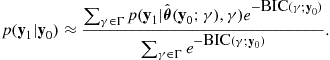 (25.41)
Although such a mixture often outperforms a single best model when used to make predictions about future data [38], there are several drawbacks to the model averaging approach. The first is that the resulting density lacks the property of parsimonity, as no model is excluded from the mixture, and therefore all model parameters contribute to the mixture. In the case of linear regression, for example, this means the ability to decide whether particular covariates are “relevant” is lost. The second drawback is that the predictive density (25.41) is in general not of the same form as any its component models, which can lead to interpretability issues.
1.25.3.3 Example application: linear regression
We conclude our examination of the BIC with an example of an application to linear regression models. Recalling that in this context the model indicator ![]() specifies which covariates, if any, should be used from the full design matrix
specifies which covariates, if any, should be used from the full design matrix ![]() to explain the observed samples
to explain the observed samples ![]() . The BIC score for a particular covariate set
. The BIC score for a particular covariate set ![]() is given by
is given by
![]() (25.42)
(25.42)
where ![]() is the maximum likelihood estimator of the noise variance for model
is the maximum likelihood estimator of the noise variance for model ![]() , and the
, and the ![]() accounts for the fact that the variance must be estimated from the data along with the k regression parameters. The BIC score (25.42) contains the terms
accounts for the fact that the variance must be estimated from the data along with the k regression parameters. The BIC score (25.42) contains the terms ![]() which are constant with respect to
which are constant with respect to ![]() and may be omitted if the set of candidate models only consists of linear regressions; if the set
and may be omitted if the set of candidate models only consists of linear regressions; if the set ![]() also contains models from alternative classes, such as artificial neural networks, then these terms are required to fully characterize the marginal probability in comparison to this alternative class of models. The consistency property of BIC is particularly useful in this setting, as it guarantees that if the data were generated from (25.42) then as
also contains models from alternative classes, such as artificial neural networks, then these terms are required to fully characterize the marginal probability in comparison to this alternative class of models. The consistency property of BIC is particularly useful in this setting, as it guarantees that if the data were generated from (25.42) then as ![]() , minimising the BIC score will recover the true model, and thus determine exactly which covariates are associated with
, minimising the BIC score will recover the true model, and thus determine exactly which covariates are associated with ![]() .
.
Given the assumption of Gaussian noise, the Bayesian mixture distribution is a weighted mixture of Gaussian distributions and thus has a particularly simple conditional mean. Let ![]() denote a
denote a ![]() vector with entries
vector with entries
that is, the vector ![]() contains the maximum likelihood estimates for the covariates in
contains the maximum likelihood estimates for the covariates in ![]() , and zeros for those covariates that are not in
, and zeros for those covariates that are not in ![]() . Then, the conditional mean of the predictive density for future data with design matrix
. Then, the conditional mean of the predictive density for future data with design matrix ![]() , conditional on an observed sample
, conditional on an observed sample ![]() , is simply a linear combination of the
, is simply a linear combination of the ![]()
![]()
which is essentially a linear regression with a special coefficient vector. While this coefficient vector will be dense, in the sense that none of its entries will be exactly zero, it retains the high degree of interpretibility that makes linear regression models so attractive.
1.25.3.4 Priors for the model structure 
One of the primary assumptions made in the derivation of the BIC is that the effects of the prior distribution for the model, ![]() , can be safely neglected. However, in some cases the number of models contained in
, can be safely neglected. However, in some cases the number of models contained in ![]() is very large relative to the sample size, or may even grow with growing sample size, and this assumption may no longer be valid. An important example is that of regression models in the context of genetic datasets; in this case, the number of covariates is generally several orders of magnitude greater than the number of samples. In this case, it is possible to use a modified BIC of the form
is very large relative to the sample size, or may even grow with growing sample size, and this assumption may no longer be valid. An important example is that of regression models in the context of genetic datasets; in this case, the number of covariates is generally several orders of magnitude greater than the number of samples. In this case, it is possible to use a modified BIC of the form
![]() (25.43)
(25.43)
which requires specification of the prior distribution ![]() . In the setting of regression models, there are two general flavors of prior distributions for
. In the setting of regression models, there are two general flavors of prior distributions for ![]() depending on the structure represented by
depending on the structure represented by ![]() . The first case is that of nested model selection. A nested model class has the important property that all models with k parameters contain all models with less than k parameters as special cases. A standard example of this is polynomial regression in which the model selection criterion must choose the order of the polynomial. A uniform prior over
. The first case is that of nested model selection. A nested model class has the important property that all models with k parameters contain all models with less than k parameters as special cases. A standard example of this is polynomial regression in which the model selection criterion must choose the order of the polynomial. A uniform prior over ![]() is an appropriate, and standard, choice of prior for nested model classes. Use of such a prior in (25.43) inflates the BIC score by a term of
is an appropriate, and standard, choice of prior for nested model classes. Use of such a prior in (25.43) inflates the BIC score by a term of ![]() ; this term is constant for all
; this term is constant for all ![]() , and may consequently be ignored when using the BIC scores to rank the models.
, and may consequently be ignored when using the BIC scores to rank the models.
In contrast, the second general case, known as all-subsets regression, is less straightforward. In this setting, there are q covariates, and ![]() contains all possible subsets of
contains all possible subsets of ![]() . This implies that the model class is no longer nested. It is tempting to assume a uniform prior over the members of
. This implies that the model class is no longer nested. It is tempting to assume a uniform prior over the members of ![]() , as this would appear to be an uninformative choice. Unfortunately, such a prior is heavily biased towards subsets containing approximately half of the covariates. To see this, note that
, as this would appear to be an uninformative choice. Unfortunately, such a prior is heavily biased towards subsets containing approximately half of the covariates. To see this, note that ![]() contains a total of
contains a total of ![]() subsets that include k covariates. This number may be extremely large when k is close to
subsets that include k covariates. This number may be extremely large when k is close to ![]() , even for moderate q, and thus these subsets will be given a large proportion of the prior probability. For example, if
, even for moderate q, and thus these subsets will be given a large proportion of the prior probability. For example, if ![]() then
then ![]() and
and ![]() . Practically, this means that subsets with
. Practically, this means that subsets with ![]() covariates are given approximately one-fifth of the total prior probability; in contrast, subsets with a single covariate receive less than one percent of the prior probability. To address this issue, an alternative approach is to use a prior which assigns equal prior probability to each set of subsets of k covariates, for all k, that is,
covariates are given approximately one-fifth of the total prior probability; in contrast, subsets with a single covariate receive less than one percent of the prior probability. To address this issue, an alternative approach is to use a prior which assigns equal prior probability to each set of subsets of k covariates, for all k, that is,
![]() (25.44)
(25.44)
This prior (or ones very similar) also arise from both empirical Bayes [39] and information theoretic arguments [27,40], and have been extensively studied by Scott and Berger [41]. This work has demonstrated that priors of the form (25.44) help Bayesian procedures overcome the difficulties associated with all-subsets model selection that adversely affect distance based criteria such as AIC and KIC [14].
In fact, Chen and Chen [42] have proposed a generalization of this prior as part of what they call the “extended BIC.” An important (specific) result of this work is the proof that using the prior (25.44) relaxes conditions required for the consistency of the BIC. Essentially, the total number of covariates may now be allowed to depend on the sample size n in the sense that ![]() , where
, where ![]() is a constant satisfying
is a constant satisfying ![]() , implying that
, implying that ![]() grows with increasing n. Then, under certain identifiability conditions on the complete design matrix
grows with increasing n. Then, under certain identifiability conditions on the complete design matrix ![]() detailed in [42], and assuming that
detailed in [42], and assuming that ![]() , the BIC given by (25.43) using the prior (25.44) almost surely selects the true model
, the BIC given by (25.43) using the prior (25.44) almost surely selects the true model ![]() as
as ![]() .
.
1.25.3.5 Markov-Chain Monte-Carlo Bayesian methods
We conclude this section by briefly discussing several alternative approaches to Bayesian model selection based on random sampling from the posterior distribution, ![]() , which fall under the general umbrella of Markov Chain Monte Carlo (MCMC) methods [43]. The basic idea is to draw a sample of parameter values from the posterior distribution, using a technique such as the Metropolis-Hastings algorithm [44,45] or the Gibbs sampler [46,47]. These techniques are in general substantially more complex than the information criteria based approaches, both computationally and in terms of implementation,and this complexity generally brings with it greater flexibility in the specification of prior distributions as well as less stringent operating assumptions.
, which fall under the general umbrella of Markov Chain Monte Carlo (MCMC) methods [43]. The basic idea is to draw a sample of parameter values from the posterior distribution, using a technique such as the Metropolis-Hastings algorithm [44,45] or the Gibbs sampler [46,47]. These techniques are in general substantially more complex than the information criteria based approaches, both computationally and in terms of implementation,and this complexity generally brings with it greater flexibility in the specification of prior distributions as well as less stringent operating assumptions.
The most obvious way to apply MCMC methods to Bayesian model selection is through direct evaluation of the marginal (25.29). Unfortunately, this is a very difficult problem in general, and the most obvious approach, the so called harmonic mean estimator, suffers from statistical instability and convergence problems and should be avoided. In the particular case that Gibbs sampling is possible, and that the posterior is unimodal, Chib [48] has provided an algorithm to compute the approximate marginal probability from posterior samples.
An alternative to attempting to directly compute the marginal probability is to view the model indicator ![]() as the parameter of interest and randomly sample from the posterior
as the parameter of interest and randomly sample from the posterior ![]() . This allows for the space of models
. This allows for the space of models ![]() to be explored by simulation, and approximate posterior probabilities for each of the models to be determined by the frequency at which a particular model appears in the sample. There have been a large number of papers published that discuss this type of approach, and important contributions include the reversible jump MCMC algorithm of Green [49], the stochastic search variable selection algorithm [50], the shotgun stochastic search algorithm [51], and an interesting paper from Casella and Moreno [28] that combines objective Bayesian priors with a stochastic search procedure for regression models.
to be explored by simulation, and approximate posterior probabilities for each of the models to be determined by the frequency at which a particular model appears in the sample. There have been a large number of papers published that discuss this type of approach, and important contributions include the reversible jump MCMC algorithm of Green [49], the stochastic search variable selection algorithm [50], the shotgun stochastic search algorithm [51], and an interesting paper from Casella and Moreno [28] that combines objective Bayesian priors with a stochastic search procedure for regression models.
Finally, there has been a large amount of recent interest in using regularisation and “sparsity inducing” priors to combine Bayesian model selection with parameter estimation. In this approach, special priors over the model parameters are chosen that concentrate prior probability on “sparse” parameter vectors, that is, parameter vectors in which some of the elements are exactly zero. These methods have been motivated by the Bayesian connections with non-Bayesian penalized regression procedures such as the non-negative garotte [52] and the LASSO [53]. A significant advantage of this approach is that one needs only to sample from, or maximize over, the posterior of a single model containing all parameters of interest, and there is no requirement to compute marginal probabilities or to explore discrete model spaces. This is a rapidly growing area of research, and some important contributions of note include the relevance vector machine [54], Bayesian artificial neural networks [55] and the Bayesian LASSO [56,57].
1.25.4 Model selection by compression
This section examines the minimum message length (MML) (see Section 1.25.4.1) and minimum description length (MDL) (see Section 1.25.4.6) principles of model selection. Unlike the aforementioned distance based criteria, the MML and MDL principles are based on information theory and data compression. Informally, given a dataset and a set of candidate models, both MML and MDL advocate choosing the model that yields the briefest encoding of a hypothetical message comprising the model and the data. This optimal model is the simplest explanation of the data amongst the set of competing models. In this fashion, MML and MDL treat codelengths of compressed data as a measure of model complexity and, therefore, a yardstick for evaluating the explanatory power of competing models. Since data compression is equivalent to statistical learning of regularity in the data, this is intuitively a sensible procedure. It is important to note that one does not need to encode the models or the data in order to do MML and MDL inference. All that is required is to be able to calculate codelengths which can then be used for model comparison. Before discussing how MML and MDL compute codelengths of models and data, a brief discussion of information theory is necessary. For a detailed treatment of information theory, the interested reader is recommended [58].
To aid in understanding the fundamental information theory concepts, it is helpful to consider the following hypothetical scenario. There exists a sender who is transmitting a data set (message) to a receiver over a transmission channel. The receiver does not know the content of the message. The message, ![]() , is recorded using some alphabet
, is recorded using some alphabet ![]() , such as a subset of the English alphabet
, such as a subset of the English alphabet ![]() , and comprises a sequence of symbols formed from
, and comprises a sequence of symbols formed from ![]() ; for example, the message using
; for example, the message using ![]() may be
may be ![]() . The transmission channel is noiseless and does not modify transmissions in any fashion. Without loss of generality, we assume the coding alphabet used on the transmission channel is the binary alphabet
. The transmission channel is noiseless and does not modify transmissions in any fashion. Without loss of generality, we assume the coding alphabet used on the transmission channel is the binary alphabet ![]() . Prior to sending the message, the sender and the receiver agree on a suitable codebook which will be used to transmit all messages on this channel. The codebook is a mapping
. Prior to sending the message, the sender and the receiver agree on a suitable codebook which will be used to transmit all messages on this channel. The codebook is a mapping ![]() from the source alphabet
from the source alphabet ![]() to the target alphabet
to the target alphabet ![]() , where
, where ![]() is the set of all strings obtained by concatenating elements of
is the set of all strings obtained by concatenating elements of ![]() . Some possible codebooks are:
. Some possible codebooks are:
![]() (25.45)
(25.45)
![]() (25.46)
(25.46)
![]() (25.47)
(25.47)
For example, if the codebook ![]() (25.45) is used by the sender, the message
(25.45) is used by the sender, the message ![]() is mapped to the target code
is mapped to the target code ![]() . If the sender uses codebook
. If the sender uses codebook ![]() instead, the message is encoded as
instead, the message is encoded as ![]() . The task of the sender and receiver is to choose a codebook such that the transmitted message is uniquely decodable by the receiver and as brief as possible.
. The task of the sender and receiver is to choose a codebook such that the transmitted message is uniquely decodable by the receiver and as brief as possible.
If the codebook ![]() possess the prefix property, a message transmitted using
possess the prefix property, a message transmitted using ![]() is uniquely decodable requiring no delimiters between successive symbols. The prefix property states that no codeword is a prefix of any other codeword. In the above example, codebooks
is uniquely decodable requiring no delimiters between successive symbols. The prefix property states that no codeword is a prefix of any other codeword. In the above example, codebooks ![]() and
and ![]() possess the prefix property, while codebook
possess the prefix property, while codebook ![]() does not as the code 0 for source symbol a is a prefix to both codes 01 and 001. Since there exist infinitely many prefix codes, the sender and the receiver may choose the prefix code that results in the briefest possible encoding of the message
does not as the code 0 for source symbol a is a prefix to both codes 01 and 001. Since there exist infinitely many prefix codes, the sender and the receiver may choose the prefix code that results in the briefest possible encoding of the message ![]() . Intuitively, symbols in the message that appear more frequently should be assigned smaller codewords, while symbols that are very rare can be given longer codewords in order to reduce the average length of the encoding. This optimization problem is now formally explored. Note, that in the rest of the section we only consider codebooks which are uniquely decodable and possess the prefix property.
. Intuitively, symbols in the message that appear more frequently should be assigned smaller codewords, while symbols that are very rare can be given longer codewords in order to reduce the average length of the encoding. This optimization problem is now formally explored. Note, that in the rest of the section we only consider codebooks which are uniquely decodable and possess the prefix property.
Let X denote a discrete random variable defined over the support (source alphabet) ![]() with probability distribution function
with probability distribution function ![]() . The random variable X represents the sender of the message. Furthermore, let
. The random variable X represents the sender of the message. Furthermore, let ![]() denote the codelength function which gives the codeword length for each symbol in the source alphabet
denote the codelength function which gives the codeword length for each symbol in the source alphabet ![]() . For example,
. For example, ![]() bit for the codebook
bit for the codebook ![]() , while
, while ![]() bits, for the codebook
bits, for the codebook ![]() . The average codelength per symbol from source alphabet
. The average codelength per symbol from source alphabet ![]() with probability distribution function
with probability distribution function ![]() is defined as
is defined as
![]() (25.48)
(25.48)
where ![]() denotes the expected value of a random variable. We wish to choose the function
denotes the expected value of a random variable. We wish to choose the function ![]() such that the codelength for data from the random variable X is on average the shortest possible; that is we seek a function
such that the codelength for data from the random variable X is on average the shortest possible; that is we seek a function ![]() that minimises
that minimises
![]() (25.49)
(25.49)
The solution to this optimization problem is
![]() (25.50)
(25.50)
which is the Shannon information of a random variable [59]. The unit of information is derived from the base of the logarithm; commonly binary and natural logarithms are used corresponding to the bit and the nit (nat) units respectively. In the rest of this section, all logarithms are assumed to be natural logarithms, unless stated otherwise.
The Shannon information agrees with the previous intuition that high probability symbols should be assigned shorter codewords, while low probability symbols should be given longer code words. At first, it may seem troubling that Shannon information allows for non-integer length codewords. After all, how does one encode and transmit symbols of length, say, 0.2 of a nit? However, this is not an issue in practice as there exist sophisticated coding algorithms, such as arithmetic codes [60], that allow for efficient encoding in the presence of non-integer codewords. It is important to re-iterate here that MML and MDL model selection does not require any actual encoding of data to be performed; all that is required is a function to compute codelengths for data and models. Model selection is then performed by computing codelengths for all candidate models and choosing the one with the smallest codelength as optimal.
The minimum possible average codelength per symbol for a discrete random variable X is known as the Shannon entropy of X and is defined as
![]() (25.51)
(25.51)
with the convention that ![]() ; since
; since ![]() as
as ![]() , this is reasonable. The entropy of a random variable is always non-negative,
, this is reasonable. The entropy of a random variable is always non-negative, ![]() , and is a measure of uncertainty in the random variable. The maximum entropy is attained when there is maximum uncertainty in X, that is, when X is uniformly distributed over the support
, and is a measure of uncertainty in the random variable. The maximum entropy is attained when there is maximum uncertainty in X, that is, when X is uniformly distributed over the support ![]() . For example, the entropy of a random variable X with support
. For example, the entropy of a random variable X with support ![]() and probability distribution function
and probability distribution function
![]() (25.52)
(25.52)
is approximately 2.585 bits or 1.792 nits. As an another example, the entropy of random variable X following a Geometric distribution (![]() ) with distribution function
) with distribution function
![]() (25.53)
(25.53)
is given by
![]() (25.54)
(25.54)
where ![]() for
for ![]() , and
, and ![]() as
as ![]() .
.
The entropy of a random variable is the minimum average codelength per symbol with the length of each codeword X given by ![]() . By the law of large numbers, it can also be shown that using codelengths of the form
. By the law of large numbers, it can also be shown that using codelengths of the form ![]() results in a code that is optimal not only on average, but also optimal for the actually generated sequences of data. It is of interest to quantify the inefficiency resulting from encoding symbols generated by
results in a code that is optimal not only on average, but also optimal for the actually generated sequences of data. It is of interest to quantify the inefficiency resulting from encoding symbols generated by ![]() using an alternative distribution function
using an alternative distribution function ![]() , where
, where ![]() for at least one
for at least one ![]() . The extra number of nits (or bits) required per symbol on average if
. The extra number of nits (or bits) required per symbol on average if ![]() is used instead of
is used instead of ![]() is given by the Kullback-Leibler (KL) divergence (see Section 1.25.2). The KL divergence is always non-negative, and is only equal to zero when
is given by the Kullback-Leibler (KL) divergence (see Section 1.25.2). The KL divergence is always non-negative, and is only equal to zero when ![]() , for all
, for all ![]() . In words, the briefest encoding for data from source
. In words, the briefest encoding for data from source ![]() is achieved using
is achieved using ![]() as the coding distribution and any other distribution, say
as the coding distribution and any other distribution, say ![]() , will necessarily result in messages with a longer average codelength.
, will necessarily result in messages with a longer average codelength.
Recall that both MML and MDL seek models that result in the shortest codelength of a hypothetical message comprising the observed data and the model. That is, both MML and MDL seek models that result in the best compression of the observed data. Formally, this is a sensible procedure since the set of compressible strings from any data source is in fact quite small in comparison to incompressible strings from the same source. This is quantified by the following no hypercompression inequality (p. 136 [61]). Given a sample of n data points ![]() generated from a probability distribution
generated from a probability distribution ![]() , the probability of compressing
, the probability of compressing ![]() by any code is
by any code is
![]() (25.55)
(25.55)
In words, the inequality states that the probability of compressing ![]() by K bits using any code is small and decreases exponentially with increasing K. Clearly, the sender and the receiver would like K to be as large as possible leading to the briefest encoding of the observed data. For any moderate K, it is highly unlikely for a random model to result in a compression of K-bits as the number of models that can compress the data in such a manner is vanishingly small with K. In the next section, we examine model selection with the minimum message principle which is based on information theory and data compression.
by K bits using any code is small and decreases exponentially with increasing K. Clearly, the sender and the receiver would like K to be as large as possible leading to the briefest encoding of the observed data. For any moderate K, it is highly unlikely for a random model to result in a compression of K-bits as the number of models that can compress the data in such a manner is vanishingly small with K. In the next section, we examine model selection with the minimum message principle which is based on information theory and data compression.
1.25.4.1 Minimum message length (MML)
The Minimum Message Length (MML) principle for model selection was introduced by Wallace [27] and collaborators in the late 1960s [33], and has been continuously refined in the following years [62,63]. The MML principle connects the notion of compression with statistical inference, and uses this connection to provide a unified framework for model selection and parameter estimation. Recalling the transmitter-receiver framework outlined in Section 1.25.4, consider the problem of efficiently transmitting some observed data ![]() from the transmitter to the receiver. Under the MML principle, the model that results in the shortest encoding of a decodable message comprising the model and data is considered optimal. For this message to be decodable, the receiver and the transmitter must agree on a common language prior to any data being transmitted. In the MML framework, the common knowledge is a set of parametric models
from the transmitter to the receiver. Under the MML principle, the model that results in the shortest encoding of a decodable message comprising the model and data is considered optimal. For this message to be decodable, the receiver and the transmitter must agree on a common language prior to any data being transmitted. In the MML framework, the common knowledge is a set of parametric models ![]() , each comprising a set of distributions
, each comprising a set of distributions ![]() indexed by
indexed by ![]() , and a prior distribution
, and a prior distribution ![]() . The use of a subjective prior distribution means that MML is an unashamedly Bayesian principle built on information theoretic foundations.
. The use of a subjective prior distribution means that MML is an unashamedly Bayesian principle built on information theoretic foundations.
Given a model from ![]() and a prior distribution
and a prior distribution ![]() over
over ![]() we may define an (implicit) prior probability distribution,
we may define an (implicit) prior probability distribution, ![]() , on the n-dimensional data space
, on the n-dimensional data space ![]() . This distribution
. This distribution ![]() , called the marginal distribution of the data, characterizes the probability of observing any particular data set
, called the marginal distribution of the data, characterizes the probability of observing any particular data set ![]() given our choice of prior beliefs reflected by
given our choice of prior beliefs reflected by ![]() , and plays an important role in conventional Bayesian inference (see Section 1.25.3). The marginal distribution is
, and plays an important role in conventional Bayesian inference (see Section 1.25.3). The marginal distribution is
![]() (25.56)
(25.56)
The receiver and the transmitter both have knowledge of the prior density ![]() and the likelihood function
and the likelihood function ![]() , and therefore the marginal distribution. Under the assumption that our prior beliefs accurately reflect the unknown process that generated the data
, and therefore the marginal distribution. Under the assumption that our prior beliefs accurately reflect the unknown process that generated the data ![]() , the average length of the shortest message that communicates the data
, the average length of the shortest message that communicates the data ![]() to the receiver using the model
to the receiver using the model ![]() is the entropy of
is the entropy of ![]() . The marginal distribution is then used to construct a codebook for the data resulting in a decodable message with codelength
. The marginal distribution is then used to construct a codebook for the data resulting in a decodable message with codelength
![]() (25.57)
(25.57)
This is the most efficient encoding of the data using the model ![]() under the assumed likelihood function and prior density. While the marginal distribution is commonly used in Bayesian inference for model selection (as discussed in Section 1.25.3), the fact that the parameter vector
under the assumed likelihood function and prior density. While the marginal distribution is commonly used in Bayesian inference for model selection (as discussed in Section 1.25.3), the fact that the parameter vector ![]() is integrated out means that it may not be used to make inferences about the particular distribution in
is integrated out means that it may not be used to make inferences about the particular distribution in ![]() that generated the data. That is, the message does not convey anything about the quality of any particular distribution in
that generated the data. That is, the message does not convey anything about the quality of any particular distribution in ![]() in regards to encoding the observed data and cannot be used for point estimation. Following Wallace ([27], pp. 152–153), we shall refer to this code as the non-explanation code for the data.
in regards to encoding the observed data and cannot be used for point estimation. Following Wallace ([27], pp. 152–153), we shall refer to this code as the non-explanation code for the data.
In the MML framework, the message transmitting the observed data comprises two components, commonly named the assertion and the detail. The assertion is a codeword naming a particular distribution indexed by ![]() from the model
from the model ![]() , rather than a range of possible distributions in
, rather than a range of possible distributions in ![]() . The detail is a codeword that states the data
. The detail is a codeword that states the data ![]() using the distribution
using the distribution ![]() that was named in the assertion. The total, joint codelength of the message is then
that was named in the assertion. The total, joint codelength of the message is then
![]() (25.58)
(25.58)
where ![]() and
and ![]() denote the length of the assertion and detail respectively. The length of the assertion measures the complexity of a particular distribution
denote the length of the assertion and detail respectively. The length of the assertion measures the complexity of a particular distribution ![]() in model
in model ![]() , while the detail length measures the quality of the fit of the distribution
, while the detail length measures the quality of the fit of the distribution ![]() to the data
to the data ![]() . Thus, the total, joint codelength automatically captures the tradeoff between model complexity and model capacity. Intuitively, a complex model with many free parameters can be tuned to fit a large range of data sets, leading to a short detail length. However, since all parameters need to be transmitted to the receiver, the length of the assertion will be long. In contrast, a simple model with few free parameters requires a short assertion, but may not fit the data well, potentially resulting in a long detail. This highlights the first defining feature of the MML principle: the measure of model complexity and model fit are both expressed in the same unit, namely the codelength. The minimum message length principle advocates choosing the model
. Thus, the total, joint codelength automatically captures the tradeoff between model complexity and model capacity. Intuitively, a complex model with many free parameters can be tuned to fit a large range of data sets, leading to a short detail length. However, since all parameters need to be transmitted to the receiver, the length of the assertion will be long. In contrast, a simple model with few free parameters requires a short assertion, but may not fit the data well, potentially resulting in a long detail. This highlights the first defining feature of the MML principle: the measure of model complexity and model fit are both expressed in the same unit, namely the codelength. The minimum message length principle advocates choosing the model ![]() and distribution
and distribution ![]() that minimises this two-part message, that is,
that minimises this two-part message, that is,
![]()
This expression highlights the second defining feature of the MML principle: minimization of the codelength is used to perform both selection of a model structure,![]() , as well as estimation of the model parameters,
, as well as estimation of the model parameters,![]() . This is in contrast to both the distance based criteria of Section 1.25.2, and the Bayesian information criterion introduced in Section 1.25.3, which only select a structure
. This is in contrast to both the distance based criteria of Section 1.25.2, and the Bayesian information criterion introduced in Section 1.25.3, which only select a structure ![]() and do not provide an explicit framework for parameter estimation. It remains to determine how one computes the codelength (25.58).
and do not provide an explicit framework for parameter estimation. It remains to determine how one computes the codelength (25.58).
In general, while the set of candidate models ![]() will usually be countable,1 the parameter space
will usually be countable,1 the parameter space ![]() for a model
for a model ![]() is commonly continuous. The continuity of
is commonly continuous. The continuity of ![]() creates a problem for the transmitter when designing a codebook for the members of
creates a problem for the transmitter when designing a codebook for the members of ![]() needed for the assertion, as valid codebooks can only be constructed from discrete distributions. This problem may be circumvented by quantizing the continuum
needed for the assertion, as valid codebooks can only be constructed from discrete distributions. This problem may be circumvented by quantizing the continuum ![]() into a discrete, countable subset
into a discrete, countable subset ![]() . Given a subset
. Given a subset ![]() we can define a distribution over
we can define a distribution over ![]() , say
, say ![]() . This distribution implicitly defines a codelength for the members of
. This distribution implicitly defines a codelength for the members of ![]() . The assertion length for stating a particular
. The assertion length for stating a particular ![]() is then
is then ![]() . The length of the detail, encoded using the distribution indexed by
. The length of the detail, encoded using the distribution indexed by ![]() is
is ![]() , which is the negative log-likelihood of the observed data
, which is the negative log-likelihood of the observed data ![]() . The question remains: how do we choose the quantisation
. The question remains: how do we choose the quantisation ![]() and the distribution
and the distribution ![]() ? The minimum message length principle specifies that the quantisation
? The minimum message length principle specifies that the quantisation ![]() and the distribution
and the distribution ![]() be chosen such that the average codelength of the resulting two-part message is minimum, the average being taken with respect to the marginal distribution. Formally, for a model
be chosen such that the average codelength of the resulting two-part message is minimum, the average being taken with respect to the marginal distribution. Formally, for a model ![]() , the MML two-part codebook solves the following minimization problem:
, the MML two-part codebook solves the following minimization problem:
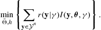 (25.59)
In the literature, this procedure is referred to as strict minimum message length (SMML) [62]. For computational reasons, the SMML procedure commonly described in the literature solves an equivalent minimization problem by partitioning the dataspace ![]() , which implicitly defines the parameter space quantisation
, which implicitly defines the parameter space quantisation ![]() and the distribution
and the distribution ![]() (for a detailed exposition the reader is referred to Chapter 3 of [27]). Model selection and parameter estimation by SMML proceeds by choosing the model/parameter pair from
(for a detailed exposition the reader is referred to Chapter 3 of [27]). Model selection and parameter estimation by SMML proceeds by choosing the model/parameter pair from ![]() and
and ![]() that results in the shortest two-part message, given
that results in the shortest two-part message, given ![]() . Interestingly, this is equivalent to performing maximum a posteriori (MAP) estimation over the quantised parameter space
. Interestingly, this is equivalent to performing maximum a posteriori (MAP) estimation over the quantised parameter space ![]() , treating
, treating ![]() as a special “quantised prior” which is implicitly defined by both the quantisation
as a special “quantised prior” which is implicitly defined by both the quantisation ![]() and the original continuous prior distribution
and the original continuous prior distribution ![]() over
over ![]() .
.
Analysis of the SMML code shows that it is approximately ![]() nits longer than the non explanation code (25.57), where k is the dimensionality of
nits longer than the non explanation code (25.57), where k is the dimensionality of ![]() (pp. 237–238, [27]). This is not surprising given that the SMML code makes a statement about the particular distribution from
(pp. 237–238, [27]). This is not surprising given that the SMML code makes a statement about the particular distribution from ![]() which was used to code the data, rather than using a mixture of distributions as in the non-explanation code. This apparent “inefficiency” in SMML allows the codelength measure to be used not only for model selection (as in the case of the non-explanation code), but also provides a theoretically sound basis for parameter estimation.
which was used to code the data, rather than using a mixture of distributions as in the non-explanation code. This apparent “inefficiency” in SMML allows the codelength measure to be used not only for model selection (as in the case of the non-explanation code), but also provides a theoretically sound basis for parameter estimation.
While the SMML procedure possesses many attractive theoretical properties (see for example, pp. 187–195 of [27] and the “false oracle” property discussed in [64]), the minimization problem (25.59) is in general NP-hard [65], and exact solutions are computationally tractable in only a few simple cases. The difficulties arise primarily due to the fact that a complete quantisation of the continuous parameter space must be found, which is a non-trivial problem that does not scale well with increasing dimensionality of ![]() . In the next section we shall examine an approximation to the two-part message length that exploits the fact that we are only interested in computing the length of the codes, rather than the codebooks. This allows us to circumvent the problematic issue of complete quantisation by using only local properties of the likelihood and prior distribution, resulting in an implementation of the MML principle that is applicable to many commonly used statistical models.
. In the next section we shall examine an approximation to the two-part message length that exploits the fact that we are only interested in computing the length of the codes, rather than the codebooks. This allows us to circumvent the problematic issue of complete quantisation by using only local properties of the likelihood and prior distribution, resulting in an implementation of the MML principle that is applicable to many commonly used statistical models.
1.25.4.2 The Wallace-Freeman message length approximation (MML87)
To circumvent the problem of determining a complete quantisation of the parameter space, Wallace and Freeman [63] presented a formula that gives an approximate length of the two-message for a particular ![]() and data set
and data set ![]() . Rather than finding an optimal quantisation for the entire parameter space
. Rather than finding an optimal quantisation for the entire parameter space ![]() , the key idea underlying their approach is to find an optimal local quantisation for the particular
, the key idea underlying their approach is to find an optimal local quantisation for the particular ![]() named in the assertion. The important implication of this approach is that the quantisation, and therefore the resulting message length formula, depends only on the particular
named in the assertion. The important implication of this approach is that the quantisation, and therefore the resulting message length formula, depends only on the particular ![]() that is of interest. Under certain regularity conditions, the Wallace-Freeman approximation states that the joint codelength of a distribution
that is of interest. Under certain regularity conditions, the Wallace-Freeman approximation states that the joint codelength of a distribution ![]() in model
in model ![]() , and data
, and data ![]() , is
, is
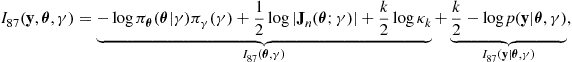 (25.60)
where ![]() is the total number of continuous, free parameters for model
is the total number of continuous, free parameters for model ![]() and
and ![]() is the Fisher information matrix for n data points given by
is the Fisher information matrix for n data points given by
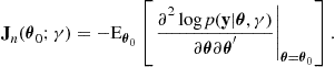 (25.61)
The quantity ![]() is the normalized second moment of an optimal quantising lattice in k-dimensions ([66]). Following ([27], p. 237), the need to determine
is the normalized second moment of an optimal quantising lattice in k-dimensions ([66]). Following ([27], p. 237), the need to determine ![]() for arbitrary dimension k is circumvented by use of the following approximation
for arbitrary dimension k is circumvented by use of the following approximation
![]()
where ![]() is the digamma function, and
is the digamma function, and ![]() . Model selection, and parameter estimation, is performed by choosing the model/parameter pair that minimises the joint codelength, that is,
. Model selection, and parameter estimation, is performed by choosing the model/parameter pair that minimises the joint codelength, that is,
![]() (25.62)
(25.62)
Unlike the SMML codelength, the MML87 codelength (25.60) is a continuous function of the continuous model parameters ![]() which makes the minimization problem (25.62) considerably easier. Again, it is important to re-iterate that unlike the distance based criteria (AIC, KIC, etc.) and the BIC, minimization of the MML87 formula yields both estimates of model structure as well as model parameters. Further, the MML87 parameter estimates possess attractive properties in comparison with estimates based on other principles such as maximum likelihood or maximum posterior mode.
which makes the minimization problem (25.62) considerably easier. Again, it is important to re-iterate that unlike the distance based criteria (AIC, KIC, etc.) and the BIC, minimization of the MML87 formula yields both estimates of model structure as well as model parameters. Further, the MML87 parameter estimates possess attractive properties in comparison with estimates based on other principles such as maximum likelihood or maximum posterior mode.
An important issue remains: under what conditions is the MML87 formula valid? In brief, the MML87 codelength is generally valid if: (i) the maximum likelihood estimates associated with the likelihood function obey the central limit theorem everywhere in ![]() , and (ii) the local curvature of the prior distribution
, and (ii) the local curvature of the prior distribution ![]() is negligible compared to the curvature of the negative log-likelihood everywhere in
is negligible compared to the curvature of the negative log-likelihood everywhere in ![]() . An important point to consider is how close the Wallace–Freeman approximate codelength is to the exact SMML codelength given by (25.59). If the regularity conditions under which the MML87 formula was derived are satisfied, then the MML87 codelength is, on average, practically indistinguishable from the exact SMML codelength (pp. 230–231, [27]).
. An important point to consider is how close the Wallace–Freeman approximate codelength is to the exact SMML codelength given by (25.59). If the regularity conditions under which the MML87 formula was derived are satisfied, then the MML87 codelength is, on average, practically indistinguishable from the exact SMML codelength (pp. 230–231, [27]).
In the particular case that the prior ![]() is conjugate2 with the likelihood
is conjugate2 with the likelihood ![]() , and depends on some parameters
, and depends on some parameters ![]() (usually referred to as “hyperparameters”), Wallace (pp. 236–237, [27]) suggested a clever modification of the MML87 formula that makes it valid even if the curvature of the prior is significantly greater than the curvature of the likelihood. The idea is to first propose some imaginary “prior data”
(usually referred to as “hyperparameters”), Wallace (pp. 236–237, [27]) suggested a clever modification of the MML87 formula that makes it valid even if the curvature of the prior is significantly greater than the curvature of the likelihood. The idea is to first propose some imaginary “prior data” ![]() whose properties depend only on the prior hyperparameters
whose properties depend only on the prior hyperparameters ![]() . It is then possible to view the prior
. It is then possible to view the prior ![]() as a posterior of the likelihood of this prior data
as a posterior of the likelihood of this prior data ![]() and some initial uninformative prior
and some initial uninformative prior ![]() that does not depend on the hyperparameters
that does not depend on the hyperparameters ![]() . Formally, we seek the decomposition
. Formally, we seek the decomposition
![]() (25.63)
(25.63)
where ![]() is the likelihood of m imaginary prior samples and
is the likelihood of m imaginary prior samples and ![]() is an uninformative prior. The new Fisher Information
is an uninformative prior. The new Fisher Information ![]() is then constructed from the new combined likelihood
is then constructed from the new combined likelihood ![]() , and the “curved prior” MML87 approximation is simply
, and the “curved prior” MML87 approximation is simply
![]() (25.64)
(25.64)
![]() (25.65)
(25.65)
This new Fisher information matrix has the interesting interpretation of being the asymptotic lower bound of the inverse of the variance of the maximum likelihood estimator using the combined data ![]() rather than for simply the observed data
rather than for simply the observed data ![]() . It is even possible in this case to treat the hyperparameters as unknown, and use an extended message length formula to estimate both the model parameters
. It is even possible in this case to treat the hyperparameters as unknown, and use an extended message length formula to estimate both the model parameters ![]() and the prior hyperparameters
and the prior hyperparameters ![]() in this hierarchical structure [67,68].
in this hierarchical structure [67,68].
What is the advantage of using the MML87 estimates over the traditional maximum likelihood and MAP estimates? In addition to possessing important invariance and consistency properties that are discussed in the next sections, there is a large body of empirical evidence demonstrating the excellent performance of the MML87 estimator in comparison to traditional estimators such as maximum likelihood and the maximum a posteriori (MAP) estimator, particularly for small to moderate sample sizes. Examples include the normal distribution [27], factor analysis [69], estimation of multiple means [67], the von Mises and spherical von Mises-Fisher distribution [70,71] (pp. 266–269, [27]) and autoregressive moving average models [72]. In the next sections we will discuss some important properties of the Wallace-Freeman approximation. For a detailed treatment of the MML87 approximation, we refer the interested reader to Chapter 5 of [27].
1.25.4.2.1 Model selection consistency
Recall from Section 1.25.3.2 that the BIC procedure yields a consistent estimate of the true, underlying model, say ![]() , that generated the data. The estimate
, that generated the data. The estimate ![]() is also a consistent estimate of
is also a consistent estimate of ![]() as
as ![]() under certain conditions. Assuming that the Fisher information matrix satisfies
under certain conditions. Assuming that the Fisher information matrix satisfies
![]() (25.66)
(25.66)
with ![]() , the MML87 codelength approximation can be rewritten as
, the MML87 codelength approximation can be rewritten as
![]() (25.67)
(25.67)
This is clearly equivalent to the well known BIC discussed in Section 1.25.3.1, and thus the estimator ![]() is consistent as
is consistent as ![]() . For a more rigorous and general proof, the reader is directed to [73].
. For a more rigorous and general proof, the reader is directed to [73].
1.25.4.2.2 Invariance
There is in general no unique way to parameterise the distributions that comprise a statistical model. For example, the normal distribution is generally expressed in terms of mean and variance parameters, say ![]() . However, the alternate parameterisations
. However, the alternate parameterisations ![]() and
and ![]() are equally valid and there is no reason, beyond ease of interpretation, to prefer any particular parameterisation. A sensible estimation procedure should be invariant to the parameterisation of the model; that is, it should give the same answer irrespective of how the inference question is framed. While the commonly used maximum likelihood estimator possesses the invariance property, both the maximum a posteriori estimator and posterior mean estimator based on the Bayesian posterior distribution
are equally valid and there is no reason, beyond ease of interpretation, to prefer any particular parameterisation. A sensible estimation procedure should be invariant to the parameterisation of the model; that is, it should give the same answer irrespective of how the inference question is framed. While the commonly used maximum likelihood estimator possesses the invariance property, both the maximum a posteriori estimator and posterior mean estimator based on the Bayesian posterior distribution ![]() given by (25.28) are not invariant. The SMML and MML87 are invariant under one-to-one reparameterisations, and thus provide an important alternative Bayesian estimation procedure.
given by (25.28) are not invariant. The SMML and MML87 are invariant under one-to-one reparameterisations, and thus provide an important alternative Bayesian estimation procedure.
1.25.4.2.3 Parameter estimation consistency
Consider the case that the data ![]() is generated by a particular distribution
is generated by a particular distribution ![]() from the model
from the model ![]() , that is,
, that is, ![]() . A sequence of estimators,
. A sequence of estimators, ![]() , of parameter
, of parameter ![]() is consistent if and only if
is consistent if and only if
![]()
for any ![]() as
as ![]() . In words, this means that as we accumulate more and more data about the parameters the estimator converges to the true parameter value
. In words, this means that as we accumulate more and more data about the parameters the estimator converges to the true parameter value ![]() . If we consider the case that the dimensionality of
. If we consider the case that the dimensionality of ![]() does not depend on n, and the Fisher information matrix satisfies (25.36) then the maximum likelihood estimator is consistent under suitable regularity conditions [74]. The consistency of the MML87 estimator in this particular case follows by noting that minimising the asymptotic message length (25.67) is equivalent to maximizing the likelihood; similar arguments can also be used to establish the consistency of the MAP and mean posterior estimators in this case.
does not depend on n, and the Fisher information matrix satisfies (25.36) then the maximum likelihood estimator is consistent under suitable regularity conditions [74]. The consistency of the MML87 estimator in this particular case follows by noting that minimising the asymptotic message length (25.67) is equivalent to maximizing the likelihood; similar arguments can also be used to establish the consistency of the MAP and mean posterior estimators in this case.
The situation is strikingly different in the case that the dimensionality of the parameter space depends on the sample size. In this setting there is usually a small number of parameters of interest for which information grows with increasing sample size, and a large number of auxiliary “nuisance” parameters for which an increasing sample size brings no new information. Maximum likelihood estimation, as well as the MAP and mean posterior estimation, of the parameters of interest is in general inconsistent. In contrast, the MML87 estimator has been shown to provide consistent estimates in the presence of many nuisance parameters in several important statistical models, including the Neyman-Scott problem [75], factor analysis [69,76] (also pp. 297–303 in [27]), multiple cutpoint estimation [77] and mixture modeling ([78] and pp. 275–297 in [27]). While a general proof of the consistency of the MML principle in the presence of nuisance parameters does not currently exist, there have been no problems studied so far in which it has failed to yield consistent estimates.
1.25.4.2.4 Similarities with Bayesian inference
There are many similarities between the minimum message length principle and the more conventional Bayesian approaches such as those discussed in Section 1.25.3 (see [79] for a detailed discussion). The differences in codelengths (MML87 or otherwise) between two models may be used to compute an approximate Bayes factor, that is,
![]()
The usual interpretations applied to regular Bayes factors apply equally well to the approximate Bayes factors determined by codelength differences. Further, the codelength measure may be used to perform model averaging over the set of candidate models ![]() in a similar fashion to BIC, as discussed in Section 1.25.3.1. In this case, we use (25.41), replacing the BIC score with the codelength, and (ideally) replacing the maximum likelihood estimate with the appropriate minimum message length estimate.
in a similar fashion to BIC, as discussed in Section 1.25.3.1. In this case, we use (25.41), replacing the BIC score with the codelength, and (ideally) replacing the maximum likelihood estimate with the appropriate minimum message length estimate.
1.25.4.3 Other message length approximations
Recently, Schmidt [72,80] introduced a new codelength approximation that can be used for models for which the application of the Wallace-Freeman approximation is problematic. The new approximation, called MML08, is more computationally tractable than the strict MML procedure, but requires evaluation of sometimes difficult integrals. The joint MML08 codelength of data ![]() and parameters
and parameters ![]() , for model
, for model ![]() , is given by
, is given by
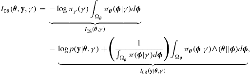 (25.68)
where ![]() is the Kullback-Leibler divergence and
is the Kullback-Leibler divergence and ![]() is chosen to minimise the codelength. The MML08 is a generalization of the previously proposed MMLD codelength approximation [81,82] and is invariant under transformations of the parameters. The MML08 approximation has been applied to the problem of order selection for autoregressive moving average models [72]. Efficient algorithms to compute approximate MMLD and MML08 codelengths are given in [72,83,84].
is chosen to minimise the codelength. The MML08 is a generalization of the previously proposed MMLD codelength approximation [81,82] and is invariant under transformations of the parameters. The MML08 approximation has been applied to the problem of order selection for autoregressive moving average models [72]. Efficient algorithms to compute approximate MMLD and MML08 codelengths are given in [72,83,84].
1.25.4.4 Example: MML linear regression
We continue our running example by applying the minimum message length principle to the selection of covariates in the linear regression model. By choosing different prior distributions for the coefficients ![]() we can arrive at many different MML criteria (for example, [85,86] and pp. 270–272, [27]); however, provided the chosen prior distribution is not unreasonable all codelength criteria will perform approximately equivalently, particularly for large sample sizes. Two recent examples of MML linear regression criteria, called “MMLu” and “MMLg,” that do not require the specification of any subjective prior information are given in [68]. The MMLu criterion exploits some properties of the linear model with Gaussian noise to derive a data driven, proper uniform prior for the regression coefficients. Recall that in the linear regression case, the model index
we can arrive at many different MML criteria (for example, [85,86] and pp. 270–272, [27]); however, provided the chosen prior distribution is not unreasonable all codelength criteria will perform approximately equivalently, particularly for large sample sizes. Two recent examples of MML linear regression criteria, called “MMLu” and “MMLg,” that do not require the specification of any subjective prior information are given in [68]. The MMLu criterion exploits some properties of the linear model with Gaussian noise to derive a data driven, proper uniform prior for the regression coefficients. Recall that in the linear regression case, the model index ![]() specifies the covariates to be used from the full design matrix
specifies the covariates to be used from the full design matrix ![]() . For a given
. For a given ![]() , the MMLu codelength for a linear regression model is
, the MMLu codelength for a linear regression model is
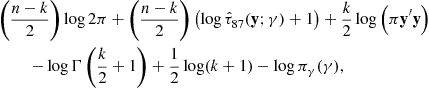 (25.69)
where the MMLu parameter estimates are given by
![]() (25.70)
(25.70)
![]() (25.71)
(25.71)
Here, ![]() denotes the number of covariates in the regression model
denotes the number of covariates in the regression model ![]() is a suitable prior for the model index (see Section 1.25.3.4 for a discussion of suitable priors), and
is a suitable prior for the model index (see Section 1.25.3.4 for a discussion of suitable priors), and
![]() (25.72)
(25.72)
is the fitted sum-of-squares for the least-squares estimates (25.5). Due to the use of a uniform prior on the regression coefficients, and the nature of the Fisher information matrix, the MML87 estimates of the regression coefficients coincide with the usual maximum likelihood estimates (25.5). In contrast to the maximum likelihood estimate of ![]() , given by (25.6), the MML87 estimate is exactly unbiased even for finite sample sizes n.
, given by (25.6), the MML87 estimate is exactly unbiased even for finite sample sizes n.
The MMLg criterion further demonstrates the differences in parameter estimation that are possible by using the MML principle. This criterion is based on a special hierarchical Gaussian prior, and uses some recent extensions to the MML87 codelength to estimate the parameters of the prior distribution in addition to the regression coefficients [67]. For a given ![]() , the MMLg codelength for a linear regression model is
, the MMLg codelength for a linear regression model is
![]() (25.73)
(25.73)
where ![]() . This formula is applicable only when
. This formula is applicable only when ![]() , and
, and ![]() , where
, where
![]()
and ![]() is the positive-part function. The codelength for a “null” model (
is the positive-part function. The codelength for a “null” model (![]() ) is given by
) is given by
![]() (25.74)
(25.74)
We note that (25.73) corrects a minor mistake in the simplified form of MMLg in [68], which erroneously excluded the additional “![]() ” term. The MMLg estimates of
” term. The MMLg estimates of ![]() and
and ![]() are given by
are given by
![]() (25.75)
(25.75)
![]() (25.76)
(25.76)
which are closely related to the unbiased estimate (25.70) of ![]() used by the MMLu criterion. The MMLg estimates of the regression coefficients
used by the MMLu criterion. The MMLg estimates of the regression coefficients ![]() are the least-squares estimates scaled by a quantity less than unity which is called a shrinkage factor [87]. This factor depends crucially on the estimated strength of the noise variance and signal strength, and if the noise variance is too large,
are the least-squares estimates scaled by a quantity less than unity which is called a shrinkage factor [87]. This factor depends crucially on the estimated strength of the noise variance and signal strength, and if the noise variance is too large, ![]() and the coefficients are completely shrunk to zero (that is, none of the covariates are deemed associated with the observations). Further, it turns out that the MMLg shrinkage factor is optimal in the sense that for
and the coefficients are completely shrunk to zero (that is, none of the covariates are deemed associated with the observations). Further, it turns out that the MMLg shrinkage factor is optimal in the sense that for ![]() , the shrunken estimates of
, the shrunken estimates of ![]() will, on average, be better at predicting future data arising from the same source than the corresponding least squares estimates [88].
will, on average, be better at predicting future data arising from the same source than the corresponding least squares estimates [88].
1.25.4.5 Applications of MML
The MML principle has been applied to a large number statistical models. Below is an inexhaustive list of some of the many successful applications of MML; a more complete list may be found in [82].
• Mixture modeling [33,78,89].
• Decision trees/graphs [90–92].
• Artificial neural networks [95,96].
• Linear Regression [68,85,86,97].
• Autoregressive moving average (ARMA) models [72,98,99].
Detailed derivations of the message length formulas for many of these models, along with discussions of their behavior, can also be found in Chapters 6 and 7 of [27].
1.25.4.6 The minimum description length (MDL) principle
The minimum description length (MDL) principle [101,102] was independently developed by Jorma Rissanen from the late 1970s [32,103,104], and embodies the same idea of statistical inference via data compression as the MML principle. While there are many subtle, and not so subtle, differences between MML and MDL, the most important is the way in which they view prior distributions (for a comparison of early MDL and MML, see [105]). The MDL principle views prior distributions purely as devices with which to construct codelengths, and the bulk of the MDL research has been focused on finding ways in which the specification of subjective prior distributions may be avoided. In the MML principle, the codebook is constructed to minimise the average codelength of data drawn from the marginal distribution, which captures our prior beliefs about the data generating source. The MDL principle circumvents the requirement to explicitly specify prior beliefs, and instead appeals to the concept of minimising the worst-case behavior of the codebook. Formally, we require the notion of coding regret
![]() (25.77)
(25.77)
where ![]() is the codelength of the data
is the codelength of the data ![]() using model
using model ![]() , and
, and ![]() is the maximum likelihood estimator. As the maximum likelihood estimator minimises the codelength of the data (without stating anything about the model), the negative log-likelihood evaluated at the maximum represents an ideal target codelength for the data. Unfortunately, this is only realizable if the sender and receiver have a priori knowledge of the maximum likelihood estimator, which in an inferential setting is clearly nonsensical.
is the maximum likelihood estimator. As the maximum likelihood estimator minimises the codelength of the data (without stating anything about the model), the negative log-likelihood evaluated at the maximum represents an ideal target codelength for the data. Unfortunately, this is only realizable if the sender and receiver have a priori knowledge of the maximum likelihood estimator, which in an inferential setting is clearly nonsensical.
Clearly, one would like to keep the regret as small as possible in some sense, to ensure that the chosen codebook is efficient. The MML approach minimises average excess codelength over the marginal distribution, which requires an explicit prior distribution. To avoid this requirement, Rissanen advocates choosing a codebook that minimises the maximum (worst-case) coding regret (25.77), that is finding the probability distribution f that solves the following problem:
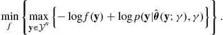 (25.78)
The solution to this optimization problem is known as the normalized maximum likelihood (NML) [106,107] (or Shtarkov [108]) distribution, and the resulting codelength is given by
![]() (25.79)
(25.79)
In MDL parlance, the second term on the right hand side of (25.79) is called the parametric complexity of the model ![]() . The parametric complexity has several interesting interpretations: (i) it is the logarithm of the normalizing constant required to render the infeasible maximum likelihood codes realizable; (ii) it is the (constant) regret obtained by the normalized maximum likelihood codes with respect to the unattainable maximum likelihood codes, and (iii) it is the logarithm of the number of distinguishable distributions contained in the model
. The parametric complexity has several interesting interpretations: (i) it is the logarithm of the normalizing constant required to render the infeasible maximum likelihood codes realizable; (ii) it is the (constant) regret obtained by the normalized maximum likelihood codes with respect to the unattainable maximum likelihood codes, and (iii) it is the logarithm of the number of distinguishable distributions contained in the model ![]() at sample size n[109]. In addition to the explicit lack of prior distributions, the NML code (25.79) differs from the MML two-part codes in the sense that it does not explicitly depend on any particular distribution in the model
at sample size n[109]. In addition to the explicit lack of prior distributions, the NML code (25.79) differs from the MML two-part codes in the sense that it does not explicitly depend on any particular distribution in the model ![]() . This means that like the marginal distribution discussed in Section 1.25.4.1, the NML codes cannot be used for point estimation of the model parameters
. This means that like the marginal distribution discussed in Section 1.25.4.1, the NML codes cannot be used for point estimation of the model parameters ![]() .
.
Practically, the normalizing integral in (25.79) is difficult to compute for many models. Rissanen has derived an asymptotic approximation to the NML distribution which is applicable to many commonly used statistical models (including for example, linear models with Gaussian noise and autoregressive moving average models) [106]. Under this approximation, the codelength formula is given by
![]() (25.80)
(25.80)
where k is the number of free parameters for the model ![]() is the sample size and
is the sample size and ![]() is the per sample Fisher information matrix given by (25.36). The approximation (25.80) swaps an integral over the dataspace for an often simpler integral over the parameter space. For models that satisfy the regularity conditions discussed in [106], the approximate NML codelength satisfies
is the per sample Fisher information matrix given by (25.36). The approximation (25.80) swaps an integral over the dataspace for an often simpler integral over the parameter space. For models that satisfy the regularity conditions discussed in [106], the approximate NML codelength satisfies
![]()
where ![]() denotes a term that disappears as
denotes a term that disappears as ![]() .
.
The NML distribution is only one of the coding methods considered by Rissanen and co-workers in the MDL principle; the interested reader is referred to Grünwald’s book [61] for a detailed discussion of the full spectrum of coding schemes developed within the context of MDL inference.
1.25.4.7 Problems with divergent parametric complexity
The NML distribution offers a formula for computing codelengths that is free of the requirement to specify suitable prior distributions, and therefore appears to offer a universal approach to model selection by compression. Unfortunately, the formula (25.79) is not always applicable as the parametric complexity can diverge, even in commonly used models [110]; this also holds for the approximate parametric complexity in (25.80). To circumvent this problem, Rissanen [106] recommends bounding either the dataspace, for (25.79), or the parameter space, for (25.80), so that the parametric complexity is finite. In the case of linear regression models with Gaussian noise, Rissanen extends this idea even further by treating the hyperparameters that specify the bounding region as parameters, and re-applying the NML formula to arrive at a parameter-free criterion (see [111] for details). Other models with infinite parametric complexity which have been addressed in a similar manner include the Poisson and geometric distributions [110] and stationary autoregressive models [112].
Unfortunately, the choice of bounding region is in general arbitrary, and different choices will lead to different codelength formulae, and hence different behavior. In this sense, the choice of bounding region is akin to the selection of a prior distribution in MML; however, advocates of the Bayesian approach argue that selection of a prior density is significantly more transparent, and interpretable, than the choice of a bounding region.
1.25.4.8 Sequential variants of MDL
One way to overcome the problems of infinite parametric complexity is to code the data sequentially. In this framework, one uses the first t datapoints, ![]() , to construct a predictive model that is used to code
, to construct a predictive model that is used to code ![]() . This process may be repeated until the entire dataset
. This process may be repeated until the entire dataset ![]() has been “transmitted”, and the resulting codelength may be used for model selection. This idea was first proposed as part of the predictive MDL procedure [101,113].
has been “transmitted”, and the resulting codelength may be used for model selection. This idea was first proposed as part of the predictive MDL procedure [101,113].
More recently, the idea has been refined with the introduction of the sequentially normalized maximum likelihood (SNML) model [114], and the related conditional normalized maximum likelihood (CNML) model [115]. These exploit the fact that the parametric complexity, conditional on some observed data, is often finite, even if the unconditional parametric complexity diverges. Additionally, the CNML distributions can be used to make predictions about future data arising from the same source in a similar manner to the Bayesian predictive distribution. A recent paper comparing SNML and CNML against Bayesian and MML approaches in the particular case of exponential distributions found that the SNML predictive distribution has favorable properties in comparison to the predictive distribution formed by “plugging in” the maximum likelihood estimates [116]. Further information on variants of the MDL principle is available in [61,102].
1.25.4.9 Relation to MML and Bayesian inference
It is of interest to compare the NML coding scheme to the codebooks advocated by the MML principle. This is most easily done by comparing the approximate NML codelength (25.80) to the Wallace-Freeman approximate codelength (25.60). Consider the so-called Jeffreys prior distribution:
 (25.81)
The normalizing term in the above equation is the approximate parametric complexity in (25.80). Substituting (25.81) into the Wallace-Freeman code (25.60) leads to the cancellation of the Fisher information term, and the resulting Wallace-Freeman codelength is within ![]() of the approximate NML codelength. This difference in codelengths is attributed to the fact that MML codes state a specific member of the set
of the approximate NML codelength. This difference in codelengths is attributed to the fact that MML codes state a specific member of the set ![]() which is used to transmit the data, while the NML distribution makes no such assertion. The close similarity between the MDL and MML codelengths was demonstrated in [116] in the context of coding data arising from exponential distributions. A further comparison of MDL, the NML distribution and MML can be found in [27], pp. 408–415.
which is used to transmit the data, while the NML distribution makes no such assertion. The close similarity between the MDL and MML codelengths was demonstrated in [116] in the context of coding data arising from exponential distributions. A further comparison of MDL, the NML distribution and MML can be found in [27], pp. 408–415.
The close equivalence of the approximate NML and Wallace-Freeman codes implies that like the BIC, the approximate NML criterion is a consistent estimator of the true model ![]() that generated the data, assuming
that generated the data, assuming ![]() , and that the normalizing integral is finite. In fact, the earliest incarnation of MDL introduced in 1978 [32] was exactly equivalent to the Bayesian information criterion, which was also introduced in 1978. This fact has caused some confusion in the engineering community, where the terms MDL and BIC are often used interchangeably to mean the “k-on-two log n” criterion given by (25.37) (this issue and its implications are discussed, for example, in [117]).
, and that the normalizing integral is finite. In fact, the earliest incarnation of MDL introduced in 1978 [32] was exactly equivalent to the Bayesian information criterion, which was also introduced in 1978. This fact has caused some confusion in the engineering community, where the terms MDL and BIC are often used interchangeably to mean the “k-on-two log n” criterion given by (25.37) (this issue and its implications are discussed, for example, in [117]).
We conclude this section with a brief discussion of the differences and similarities between the MML and MDL principles. This is done to attempt to clear up some of the confusion and misunderstands surrounding these two principles. The MDL principle encompasses a range of compression schemes (such as the NML model, the Bayesian model, etc.), which are unified by the deeper concept of universal models for data compression. In recent times, the MDL community has focused on those universal models that attain minimax regret with respect to the maximum likelihood codes to avoid the specification of subjective prior distributions. The two-part codebooks used in the MML principle are also types of universal models, and so advocates of the MDL school often suggest that MML is subsumed in the MDL principle. However, as the above coincidence of Wallace-Freeman and NML demonstrates, the MDL universal models can be implemented in the MML framework by the appropriate choice of prior distribution, and thus the MML school tend to suggest that MDL is essentially a special case of the MML theory, particularly given the time-line of developments in the two camps.
Practically, the most important difference between the two principles is in the choice of two-part (for MML) versus one-part (for MDL) coding schemes. The two-part codes chosen by MML allow for the explicit definition of new classes of parameter estimators, in addition to model selection criteria, which are not obtainable by the one-part MDL codes. As empirical, and theoretical evidence strongly supports the general improvement of the MML estimators over the maximum likelihood and Bayesian MAP estimators, this difference seems to be of perhaps the greatest importance.
1.25.4.10 Example: MDL linear regression
An MDL criterion for the linear regression example is now examined. Given the importance of linear regression, there have been a range of MDL inspired criteria developed, for example, the predictive MDL criterion [101], g-MDL [118], Liang and Barron’s approach [119], sequentially normalized least squares [120,121] and normalized maximum likelihood based methods [40,111,122]. We choose to focus on the NML criterion introduced by Rissanen in 2000 [111] as it involves no user specified hyperparameters and does not depend on the ordering of the data, a problem which affects the predictive and sequential procedures. Recall that in the linear regression case, the model index ![]() specifies which covariates are to be used from the full design matrix
specifies which covariates are to be used from the full design matrix ![]() . For a given
. For a given ![]() , the NML codelength, up to constants, is
, the NML codelength, up to constants, is
 (25.82)
where ![]() is the maximum likelihood estimate of
is the maximum likelihood estimate of ![]() given by (25.6),
given by (25.6),
![]() (25.83)
(25.83)
and ![]() are the least-squares estimates of the model coefficients
are the least-squares estimates of the model coefficients ![]() for subset
for subset ![]() given by (25.5). As in the case of the BIC given by (25.43), and the MML linear regression criteria given by (25.69) and (25.73, 25.74), the codelength includes a prior
given by (25.5). As in the case of the BIC given by (25.43), and the MML linear regression criteria given by (25.69) and (25.73, 25.74), the codelength includes a prior ![]() required to state the subset
required to state the subset ![]() , and suitable choices are discussed in Section 1.25.3.4.
, and suitable choices are discussed in Section 1.25.3.4.
Interestingly, Hansen and Yu [123] have shown that NML is either asymptotically consistent or asymptotically efficient depending on the nature of the data generating distribution. In this way, the NML criterion can be viewed as a “bridge” between the AIC-based criteria and the BIC. Given the close similarity between the NML and MML linear regression criteria [68], this property is expected to also hold for the MML linear regression criteria.
1.25.4.11 Applications of MDL
Below is an incomplete list of successful applications of the MDL principle to commonly used statistical models:
• the multinomial distribution [124],
• causal models and Naïve Bayes classification [125,126],
• variable bin-width histograms [127,128],
• linear regression [111,118,122],
• autoregressive models [112],
Of particular interest is the multinomial distribution as it is one of the few models for which the exact parametric complexity is finite without any requirement for bounding, and may be efficiently computed in polynomial time using the clever algorithm discussed in [124]. This algorithm has subsequently been used to compute codelengths in histogram estimation and other similar models.
1.25.5 Simulation
We conclude with a brief simulation demonstrating the practical application of the distance based, Bayesian and information theoretic model selection criteria discussed in this chapter. The simulation compares the AICc(25.25), KICc(25.27), BIC (25.42), MMLu(25.69), MMLg(25.73, 25.74) and NML (25.82) criteria on the problem of polynomial order selection with linear regression. Datasets of various sample sizes ![]() were generated from the polynomial model
were generated from the polynomial model
![]() (25.84)
(25.84)
with design points x uniformly generated from the compact set ![]() [13,102]. The noise variance
[13,102]. The noise variance ![]() was chosen to yield a signal-to-noise ratio of ten. Recalling the linear regression example from Section 1.25.1.2, the complete design matrix consisted of polynomial bases
was chosen to yield a signal-to-noise ratio of ten. Recalling the linear regression example from Section 1.25.1.2, the complete design matrix consisted of polynomial bases ![]() for
for ![]() ,
,
![]() (25.85)
(25.85)
For each generated data set, each of the six criteria were used to select a nested polynomial model up to the maximum polynomial of order ![]() . The simulation was repeated
. The simulation was repeated ![]() times and the zero-order polynomial model was not considered. The criteria were compared on two important metrics: (i) order selection, and (ii) squared prediction error. The results are presented in Table 25.1.
times and the zero-order polynomial model was not considered. The criteria were compared on two important metrics: (i) order selection, and (ii) squared prediction error. The results are presented in Table 25.1.
Table 25.1
Polynomial Order Selected by the Criteria (Expressed as Percentages) and Squared Error in Estimated Coefficients
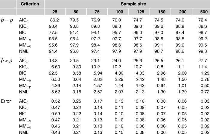
The simulation is highly illustrative of the general behaviors of the model selection criteria under consideration. For small sample sizes (![]() ), the KICc criterion performs adequately in terms of order selection, but like the AICc, this performance does not improve with increasing sample size. This is not surprising given that both AICc and KICc are not consistent model selection procedures. While BIC performs relatively poorly for the smallest sample sizes, its performance dramatically improves when the sample size is larger. The asymptotic approximation from which BIC is derived is inadequate for small sample sizes which explains its poor performance. In contrast, the MML and NML criteria perform well for all sample sizes in terms of both order selection and prediction error. In this particular example, the MMLu and NML criteria are virtually indistinguishable, while the MMLg criterion performs slightly better. For larger sample sizes
), the KICc criterion performs adequately in terms of order selection, but like the AICc, this performance does not improve with increasing sample size. This is not surprising given that both AICc and KICc are not consistent model selection procedures. While BIC performs relatively poorly for the smallest sample sizes, its performance dramatically improves when the sample size is larger. The asymptotic approximation from which BIC is derived is inadequate for small sample sizes which explains its poor performance. In contrast, the MML and NML criteria perform well for all sample sizes in terms of both order selection and prediction error. In this particular example, the MMLu and NML criteria are virtually indistinguishable, while the MMLg criterion performs slightly better. For larger sample sizes ![]() all four consistent criteria performed essentially the same.
all four consistent criteria performed essentially the same.
This brief simulation serves to demonstrate the general behavior of the six criteria and should not be taken as indicative of their performance in other model selection problems. For a more detailed comparison of some recent regression methods, including MMLu, MMLg and NML, see [122]. The MMLu, MMLg and NML criteria were found to be amongst the best of the eight criteria considered in all experiments conducted by the authors. 3
References
1. Lehmann EL, Casella G. Theory of Point Estimation, Springer Texts in Statistics. fourth ed. Springer 2003.
2. Kullback S, Leibler RA. Ann Math Stat. 1951;22:79–86.
3. Takeuchi K. Suri-Kagaku. Math Sci. 1976;153:12–18 (in Japanese).
4. Shibata R. Statistical aspects of model selection. In: Willems JC, ed. From Data to Model. New York: Springer; 1989;215–240.
5. Linhart H, Zucchini W. Model Selection. New York: Wiley; 1986.
6. Akaike H. IEEE Trans Automat Contr. 1974;19:716–723.
7. Hurvich CM, Tsai C-L. Biometrika. 1989;76:297–307.
8. Seghouane A-K, Amari S-I. IEEE Trans Neural Networks. 2007;18:97–106.
9. Seghouane A-K. Signal Process. 2010;90:217–224.
10. McQuarrie ADR, Tsai C-L. Regression and Time Series Model Selection. World Scientific 1998.
11. Jeffreys H. Proc Roy Soc Lond Ser A Math Phys Sci. 1946;186:453–461.
12. Cavanaugh JE. Stat Probab Lett. 1999;42:333–343.
13. Seghouane A-K, Bekara M. IEEE Trans Signal Process. 2004;52:3314–3323.
14. Schmidt DF, Makalic E. Lect Notes Artif Int. 2010;6464:223–232.
15. Seghouane AK. Signal Process. 2006;86:2074–2084.
16. Seghouane A-K. IEEE Trans Aero Electron Syst. 2011;47:1154–1165.
17. Seghouane AK. IEEE Trans Circ Syst Part I 2006;(53):2327–2335.
18. Hurvich CM, Simonoff JS, Tsai C-L. J Roy Stat Soc Ser B. 1998;60:271–293.
19. Bekara M, Knockaert L, Seghouane A-K, Fleury G. Signal Process. 2006;86:1400–1409.
20. Hurvich CM, Tsai C-L. Biometrika. 1998;85:701–710.
21. Murata N, Yoshizawa S, Amari S. IEEE Trans Neural Networks. 1994;5:865–872.
22. Seghouane AK, Bekara M, Fleury G. Signal Process. 2005;85:1405–1417.
23. Robert C. The Bayesian Choice: From Decision-Theoretic Foundations to Computational Implementation, Springer Texts in Statistics. Springer 2001.
24. J. Berger, L. Pericchi, in: P. Lahiri (Ed.), Model selection, vol. 38 of Lecture Notes Monograph Series, Hayward, CA: pp. 135–207.
25. Bernardo JM. J Roy Stat Soc Ser B. 1979;41:113–147.
26. Berger J, Pericchi L. J Am Stat Assoc. 1996;91:109–122.
27. Wallace CS. Statistical and Inductive Inference by Minimum Message Length, Information Science and Statistics. first ed. Springer 2005.
28. Casella G, Moreno E. J Am Stat Assoc. 2006;101:157–167.
29. Jeffreys H. The Theory of Probability. third ed. Oxford University Press 1961.
30. Kass RE, Raftery AE. J Am Stat Assoc. 1995;90:773–795.
31. Schwarz G. The Ann Stat. 1978;6:461–464.
32. Rissanen J. Automatica. 1978;14:465–471.
33. Wallace CS, Boulton DM. Comput J. 1968;11:185–194.
34. Barndorff-Nielsen OE, Cox DR. Asymptotic Techniques for Use in Statistics. New York: Chapman & Hall; 1989.
35. Haughton DMA. Ann Stat. 1988;16:342–355.
36. Rao CR, Wu Y. Biometrika. 1989;76:369–374.
37. Breiman L. Ann Stat. 1996;24:2350–2383.
38. Madigan D, Raftery AE. J Am Stat Assoc. 1994;89:1536–1546.
39. George EI, Foster DP. Biometrika. 2000;87:731–747.
40. Roos T, Myllymäki P, Rissanen J. IEEE Trans Signal Process. 2009;57:3347–3360.
41. Scott JG, Berger JO. Ann Stat. 2010;38:2587–2619.
42. Chen J, Chen Z. Biometrika. 2008;95:759–771.
43. Robert CP, Casella G. Monte Carlo Statistical Methods. Springer 2004.
44. Metropolis A, Rosenbluth M, Rosenbluth A, Teller E. J Chem Phys. 1953;21:1087–1092.
45. Hastings W. Biometrika. 1970;57:97–109.
46. Geman S, Geman D. IEEE Trans Pattern Anal Mach Int. 1984;6:721–741.
47. Casella G, George EI. Am Stat. 1992;46:167–174.
48. Chib S. J Am Stat Assoc. 1995;90:1313–1321.
49. Green PJ. Biometrika. 1995;82:711–732.
50. George EI, McCulloch RE. J Am Stat Assoc. 1993;88:881–889.
51. Hans C, Dobra A, West M. J Am Stat Assoc. 2007;102:507–516.
52. Breiman L. Technometrics. 1995;37:373–384.
53. Tibshirani R. J Roy Stat Soc Ser B. 1996;58:267–288.
54. Tipping ME. J Mach Learn Res. 2001;1:211–244.
55. Neal RM. Bayesian learning for neural networks Lecture Notes in Statistics Springer Verlag 1996.
56. Park T, Casella G. J Am Stat Assoc. 2008;103:681–686.
57. Hans C. Biometrika. 2009;96:835–845.
58. Cover TM, Thomas JA. Elements of Information Theory. second ed. Wiley-Interscience 2006.
59. Shannon CE. Bell Syst Tech J. 1948;27:379–423 and 623–656.
60. Rissanen J, Langdon JGG. IEEE Trans Info Theory. 1981;IT-27:12–23.
61. Grünwald PD. TheMinimum Description Length Principle, Adaptive Communication and Machine Learning. The MIT Press 2007.
62. Wallace C, Boulton D. Class Soc Bull. 1975;3:11–34.
63. Wallace CS, Freeman PR. J Roy Stat Soc Ser B. 1987;49:240–252.
64. Wallace CS. In: Proceedings of the International Conference on Information, Statistics and Induction in Science. World Scientific 1996;304–316.
65. Farr GE, Wallace CS. Comput J. 2002;45:285–292.
66. Conway JH, Sloane NJA. Sphere Packing, Lattices and Groups. third ed. Springer-Verlag 1998.
67. Makalic E, Schmidt DF. Stat Probab Lett. 2009;79:1155–1161.
68. D. Schmidt, E. Makalic, in: The 22nd Australasian Joint Conference on Artificial Intelligence, Melbourne, Australia, pp. 312–321.
69. Wallace CS, Freeman PR. J Roy Stat Soc Ser B. 1992;54:195–209.
70. C.S. Wallace, D. Dowe, MML estimation of the von Mises concentration parameter, Technical Report, Department of Computer Science, Monash University, 1993.
71. Dowe DL, Oliver J, Wallace C. Lect Notes Artif Int. 1996;1160:213–227.
72. D.F. Schmidt, Minimum message length inference of autoregressive moving average models, Ph.D. Thesis, Clayton School of Information Technology, Monash University, 2008.
73. Barron AR, Cover TM. IEEE Trans Info Theory. 1991;37:1034–1054.
74. L. LeCam, University of California Publications in, Statistics, vol. 11 1953.
75. D.L. Dowe, C.S. Wallace, in: Proceedings of 28th Symposium on the Interface, Computing Science and Statistics, vol. 28, Sydney, Australia, pp. 614–618.
76. C.S. Wallace, in: Proceedings of the 14th Biennial Statistical Conference, Queenland, Australia, p. 144.
77. Viswanathan M, Wallace CS, Dowe DL, Korb KB. Lect Notes Artif Int. 1999;1747:405–416.
78. Wallace CS, Dowe DL. Stat Comput. 2000;10:73–83.
79. J.J. Oliver, R.A. Baxter, MML and Bayesianism: similarities and differences, Technical Report TR 206, Department of Computer Science, Monash University, 1994.
80. D.F. Schmidt, in: Proceedings of the 5th Workshop on Information Theoretic Methods in Science and, Engineering (WITMSE-11).
81. L.J. Fitzgibbon, D.L. Dowe, L. Allison, in: Proceedings of the 19th International Conference on, Machine Learning (ICML’02), pp. 147–154.
82. Dowe DL. Comput J. 2008;51:523–560.
83. E. Makalic, Minimum message length inference of artificial neural networks, Ph.D. Thesis, Clayton School of Information Technology, Monash University, 2007.
84. E. Makalic, L. Allison, in: Proceedings of the 85th Solomonoff Memorial Conference, Melbourne, Australia.
85. M. Viswanathan, C. Wallace, in: Proceedings of the 7th Int. Workshop on Artif. Intelligence and Statistics, Ft. Lauderdale, Florida, USA, pp. 169–177.
86. G.W. Rumantir, C.S. Wallace, in: Proceedings of the 5th International Symposium on Intelligent Data Analysis (IDA 2003), vol. 2810, Springer-Verlag, Berlin, Germany, pp. 486–496.
87. W. James, C.M. Stein, in: Proceedings of the 4th Berkeley Symposium, vol. 1, University of California Press, pp. 361–379.
88. Sclove SL. J Am Stat Assoc. 1968;63:596–606.
89. Bouguila N, Ziou D. IEEE Trans Knowl Data Eng. 2006;18:993–1009.
90. Wallace CS, Patrick JD. Mach Learn. 1993;11:7–22.
91. Tan P, Dowe D. Lect Notes Artif Int. 2003;2903:269–281.
92. Tan P, Dowe D. Lect Notes Artif Int. 2006;4293:593–603.
93. C.S. Wallace, K.B. Korb, in: A. Gammerman (Ed.), Causal Models and Intelligent Data Management, Springer-Verlag, pp. 89–111.
94. J.W. Comley, D. Dowe, Minimum Message Length and Generalized Bayesian Nets with Asymmetric Languages, M.I.T. Press (MIT Press), pp. 265–294.
95. Makalic E, Allison L, Dowe DL. In: Proceedings of the IASTED International Conference on Artificial Intelligence and Applications (AIA 2003). 2003.
96. Makalic E, Allison L, Paplinski AP. In: Proceedings of the 8th Brazillian Symposium on Neural Networks (SBRN), Sao Luis, Maranhao, Brazil. 2004.
97. D.F. Schmidt, E. Makalic, Shrinkage and denoising by minimum message length, Technical Report 2008/230, Monash University, 2008.
98. L.J. Fitzgibbon, D.L. Dowe, F. Vahid, in: Proceedings of the International Conference on Intelligent Sensing and Information Processing (ICISIP), pp. 439–444.
99. D.F. Schmidt, in: Proceedings of the 85th Solomonoff Memorial Conference, Melbourne, Australia.
100. Baxter RA, Oliver JJ. Lect Notes Artif Int. 1996;1160:83–90.
101. Rissanen J. Stochastic Complexity in Statistical Inquiry. World Scientific 1989.
102. Rissanen J. Information and Complexity in Statistical Modeling, Information Science and Statistics. first ed. Springer 2007.
103. Rissanen J. Circuits, Systems, and Signal Process. 1982;1:395–396.
104. Rissanen J. Ann Stat. 1983;11:416–431.
105. R.A. Baxter, J. Oliver, MDL and MML: similarities and differences, Technical Report TR 207, Department of Computer Science, Monash University, 1994.
106. Rissanen J. IEEE Trans Info Theory. 1996;42:40–47.
107. Rissanen J. IEEE Trans Info Theory. 2001;47:1712–1717.
108. Shtarkov YM. Probl Inform Transm. 1987;23:3–17.
109. V. Balasubramanian, in: I.J.M.P.D. Grünwald, M.A. Pitt (Eds.), Advances in Minimum Description Length: Theory and Applications, MIT Press, pp. 81–99.
110. de Rooij S, Grünwald P. J Math Psychol. 2006;50:180–192.
111. Rissanen J. IEEE Trans Info Theory. 2000;46:2537–2543.
112. Schmidt DF, Makalic E. IEEE Trans Signal Process. 2011;59:479–487.
113. Dawid AP. J Roy Stat Soc Ser A. 1984;147:278–292.
114. T. Roos, J. Rissanen, in: Proceedings of the 1st Workshop on Information Theoretic Methods in Science and Engineering (WITMSE-08), Tampere International Center for, Signal Processing (Invited Paper).
115. Rissanen J, Roos T. In: Proceeding of the 2007 Information Theory and Applications Workshop (ITA-07). IEEE Press 2007;337–341. (Invited Paper).
116. Schmidt DF, Makalic E. IEEE Trans Info Theory. 2009;55:3087–3090.
117. Schmidt DF, Makalic E. IEEE Trans Signal Process. 2012;60:1508–1510.
118. Hansen MH, Yu B. J Am Stat Assoc. 2001;96:746–774.
119. Liang F, Barron A. IEEE Trans Info Theory. 2004;50:2708–2726.
120. Rissanen J, Roos T, Myllymäki P. J Multivariate Anal. 2010;101:839–849.
121. D.F. Schmidt, T. Roos, in: Proceedings of the 3rd Workshop on Information Theoretic Methods in Science and Engineering (WITMSE-10), Tampere International Center for, Signal Processing. (Invited Paper).
122. Giurcaˇneanu CD, Razavi SA, Liski A. Signal Process. 2011.
123. M. Hansen, B. Yu, in: Science and Statistics: A Festchrift for Terry Speed, of Lecture Notes—Monograph Series, vol. 40, Institute of Mathematical, Statistics, pp. 145–164.
124. Kontkanen P, Myllymäki P. Info Process Lett. 2007;103:227–233.
125. T. Mononen, P. Myllymaki, in: Proceedings of the 10th International Conference on Discovery Science, Lecture Notes in Computer Science, Sendai, Japan, vol. 4755, pp. 151–160.
126. T. Silander, T. Roos, P. Myllymäki, in: Proceedings of the 12th International Conference on Artificial Intelligence and, Statistics (AISTATS-09).
127. Rissanen J, Speed TP, Yu B. IEEE Trans Info Theory. 1992;38:315–323.
128. Kontkanen P, Myllymäki P. In: Meila M, Shen X, eds. Proceedings of the 11th International Conference on Artificial Intelligence and Statistics (AISTATS), San Juan, Puerto Rico. 2007.
129. Yang Y, Tabus I. In: IEEE International Workshop on Genomic Signal Processing and Statistics (GENSIPS). 2007;1–4.
130. Tabus I, Rissanen J, Astola J. Signal Process. 2003;83:713–727.
1A set A is countable if its members can be put into a one-to-one correspondence with the natural numbers, that is, ![]() .
.
2The use of a conjugate prior ensures that the posterior distribution of the parameters is of the same mathematical form as the conjugate prior distribution.
3Unfortunately, through no fault of the authors, the formulae for MMLg given in [122] is missing the ![]() term that is present in formula (25.73) in this tutorial. However, this has not effected the experimental results as the simulation code uses the correct formula (see Section 1.25.4.4).
term that is present in formula (25.73) in this tutorial. However, this has not effected the experimental results as the simulation code uses the correct formula (see Section 1.25.4.4).