
Day-Ahead and Real-Time Markets Simulation Methodology on Hydro Storage
Yang Gu*; Jordan Bakke†; James McCalley‡ * NRG Energy, Princeton, NJ, 08540
† Midcontinent Independent System Operator, Inc., Eagan, MN 55121
‡ Department of Electrical and Computer Engineering, Iowa State University, Ames, IA, 50011
Abstract
This chapter presents a simulation methodology that evaluates the economic performance of hydro storage system in the day-ahead (DA) and real-time (RT) markets. A long-term production cost simulation model is employed which conducts Security-Constrained Unit Commitment (SCUC) and Security-Constrained Economic Dispatch (SCED) and co-optimizes both the energy market and the ancillary services market. A novel simulation method named DA/RT interleave method is implemented in the production cost simulation model to represent the interactions between day-ahead market simulation and real-time market simulation. A unique RT market bidding strategy of hydro storage units named tiered bidding is proposed which uses the Value of Water in Storage (VWS) curve and DA market dispatch schedule/LMP to determine hydro storage units’ RT market offer curves.
1 Introduction
In the last decade, there has been significant growth in wind capacity in the United States, partly due to government subsidies/incentives, state renewable portfolio standards, wind-turbine technology advancement, and environmental concerns. While huge environmental benefits have been obtained by employing renewable power, there are great challenges for its large-scale integration due to its variability and inability to offer full capacity at peak loading conditions.
Many studies have been performed to evaluate the economic/technical viability of using various bulk energy-storage systems to manage wind-power fluctuations [1–5]. Energy-storage systems can perform energy arbitrage, provide high-value ancillary services, and enhance the stability of electric systems. As most energy-storage systems have fast-ramping capability, they are the ideal options to counterbalance wind-output variability. At high wind-penetration levels and/or imperfect wind forecasts, the value and use of energy storage increases.
Hydroelectric (hereafter called hydro) systems are one of the most economically competitive high capacity energy-storage options and the most widely used renewable-generation technology in the world [6]. There are three types of hydro units: pumped hydro units, run-of-the-river (ROR) hydro units, and what we refer to as dispatchable (or reservoir) hydro units. This chapter focuses on using large dispatchable hydro units, which have large water-storage reservoirs, to smooth the wind output and gain economic benefits from the electric market.
In 2011, MISO initiated a study called the “Manitoba Hydro Wind Synergy Study” to evaluate the economic benefits of using MH’s hydro system to facilitate large-scale wind integration in the Midwest independent transmission system operator (MISO). Manitoba hydro (MH) has 5.5 GW of installed hydro capacity (13 ROR hydro units and 2 dispatchable hydro units) and is currently looking to expand its hydro system by 2.2 GW over the next 15 years. MH is its own balancing authority and is outside of MISO’s market footprint, so MH is responsible for scheduling its generation to supply its own demand. Besides balancing its own generation and load, MH also participate in MISO’s energy and ancillary services market. While the ROR hydro units have limited dispatchability, the dispatchable hydro units can freely maneuver or adjust their power output to maximize their profits. From MISO’s perspective, MH’s dispatchable hydro units can be considered as a super-sized pumped storage hydro unit with low minimum capacity and a fast-ramping rate (ramping from 0 to maximum capacity in about 1 minute). During the peak hours when wind generation is low, MH increases the generation output of the dispatchable hydro units and sells energy to MISO; during the off-peak hours when the sufficient wind generation causes low locational marginal price (LMPs) in MISO, MH reduces the generation output of the dispatchable hydro units and purchases energy from MISO to serve its local load. When MH purchases energy from MISO to substitute its own dispatchable hydro generation, more water is stored in the storage reservoirs, which has the same effect as “pumping.”
As a product of the Manitoba Hydro Wind Synergy Study, a simulation methodology to model the long-term operations of hydro systems (especially dispatchable hydro units) in the day-ahead (DA) and real-time (RT) markets is presented in this chapter. The aim of the proposed simulation methodology is to accurately represent the way a hydro system operates in an energy and ancillary services market for a long period of time (e.g., 1 year). This simulation framework can then be used for various economic analyses on hydro systems, such as evaluating the economic effects of a market rule change or the economic benefits of investing new dispatchable hydro units and new transmission lines.
Previous technical publications proposed various approaches to optimize hydro-system dispatch using long-term LMP forecasts or LMP forecasts with hourly market simulations. Reference [2] proposed a mathematical optimization model for short-term hydro scheduling by optimizing the bids and operating strategy of hydro units; here, hydro units are considered as price-takers. Reference [3] discussed an hourly-discretized optimization algorithm to maximize the 24-hour operational profits of the wind-hydro power plant considering wind forecast uncertainties. A similar problem was also solved using the dynamic programming approach in [7]. In [8], a two-stage stochastic programing problem is formulated to jointly optimize a wind farm and a pumped-storage facility. In [9], the optimal bidding strategy of pumped hydro units in DA energy and ancillary services markets was investigated. Three bidding strategies of wind-hydro units in the DA market are investigated in [10]. In [11,12], the joint operation strategies of hydro/pumped-storage and wind/pumped-storage in energy and ancillary services market were discussed, respectively.
Compared with existing publications, the proposed framework has several features that are new or rare: 1) a value of water in storage (VWS) curve is introduced to capture the long-term opportunity cost of water in a storage reservoir; 2) a new simulation method called the DA/RT Interleave method is proposed to enable dispatchable hydro units to adjust their bids based on the VWS curve and the current water storage volume; 3) a unique bidding strategy of hydro units called tiered bidding (TB) is considered in the RT market simulation, which closely follows the way hydro-system operators act in the market; and 4) the wind/demand forecast errors between DA and RT markets and wind/demand intra-hour fluctuations are considered in the simulation process.
The remaining sections are organized as follows. Section 3 describes the detailed hydro-system model that considers the operating characteristics of different types of hydro systems. Section 4 illustrates the simulation methodology. Section 5 describes how wind units are modeled and how wind and load forecast uncertainties are considered in the model. Section 7 illustrates how the proposed methodology is implemented. The proposed methodology is applied to the whole Eastern Interconnection system and the simulation results are included in Section 7. This chapter concludes with a summary of the findings of this study in Section 8.
2 Hydro-System Model
Hydro units have special operating characteristics that require special considerations in the simulation model. This section illustrates modeling details of ROR hydro units and dispatchable hydro units and a special way to quantify the VWS reservoirs.
Since the production level of ROR hydro units is largely dictated by river flow, they are, in practice, much less dispatchable than reservoir units. Thus, we refer to the former as non-dispatchable and the latter as dispatchable. The dispatchable hydro units are the primary focus of this study. By selling energy (generating) to the market when prices are high and buying energy (pumping) from the market to substitute hydro generation when prices are low, the hydro-storage system can conduct energy arbitrage similar to the way pumped hydro units do without pumping losses.
2.1 Run-of-the-river Hydro Units
Run-of-the-river (ROR) hydro utilizes the run of the river flows for power generation. Run-of-the-river hydro either has no storage capability, or has a small storage reservoir. The power output of a ROR hydro unit is dependent on the water inflow, so the generation schedule cannot follow demand. Run-of-the-river hydro’s generation output follows the seasonal variation in river flow. From the power system operator’s point of view, the ROR hydro units are non-dispatchable.
In the proposed production cost model, each ROR hydro unit has an hourly generation schedule, which determines the maximum generation output for each hour. As many ROR units are along the same river, the cascading water flow is considered when building their hydro profiles. As hydro units have no fuel cost, only operations and maintenance costs are considered in the simulation model.
2.2 Dispatchable Hydro Units
Dispatchable hydro units have large water-storage reservoirs so their generation output can be adjusted. In our study, dispatchable hydro units in MH are used to counterbalance the wind fluctuations in MISO by adjusting their generation output.
In general, there is not sufficient water supply for a hydro unit to run throughout the year at full capacity, so hydro units are considered as energy-limited resources. For thermal generators not under take-or-pay contracts, the power level in one period is largely independent of the power level in previous periods, except as constrained by ramp rate. For dispatchable hydro units, however, the power level in one period depends on the power level in other periods due to the water inflow limit and the need to satisfy reservoir maximum and minimum limits. The inter-temporal constraints and energy limited feature of hydro generation requires consideration of multiple time steps and multiple time horizons in hydro scheduling.
3 Hydro-Unit Performance Curve
One of the key differences between a hydro unit and a thermal unit is that the hydro unit has a unique unit-performance curve. The generation output of a hydro storage unit can be expressed as a nonlinear function of the inflow of the water turbine and the water-level difference between the forebay (the water reservoir) and the tailrace (the channel that carries water away from the water turbine) [13–15]. For large reservoirs, the impact of variations of water levels in the upper reservoir can be ignored so the generation output is only dependent on water flow. The nonlinear production functions of hydro turbines cause computational burdens for long-term large-scale production cost simulations, so studies have been performed to linearize the nonlinear functions into linear segments [14,16]. In Figure 7.1, a piece-wise linearized hydro unit performance curve is presented, which closely represents the relationship between water inflow and turbine output. The x axis of the curve is the water flow that goes into the hydro turbine, while the y axis is the hydro-turbine generation output. The hydro-generator efficiency is defined as hydro-turbine generation output divided by flow. For example, when flow equals a, a hydro turbine’s overall efficiency can be obtained by dividing the corresponding turbine output in the curve by a.
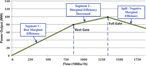
The hydro-unit performance curve is linearized into three segments, each having a different marginal efficiency. The marginal efficiency is defined as the change in hydro-turbine output as the result of one unit change in water flow, which is essentially the slope of the corresponding segment in the curve. As shown in Figure 7.1, the first segment of the unit-performance curve has the best marginal efficiency, i.e., the steepest positive slope. With the increase of water flow, the water-level difference between the forebay and the tailrace gets smaller, which decreases the efficiency of the hydro generator. The decreased marginal efficiency is shown in Figure 7.1 as segment 2 of the unit-performance curve. When the flow is at full-gate discharge and the water turbine is at maximum-rated head the maximum overall power output is achieved. If the flow keeps increasing beyond the full-gate discharge amount, the additional water needs to be released to the downstream through the spillway as the hydro turbine cannot handle the excessive water inflow. This situation is called a spill. During a spill, the water-level difference between the forebay and the tailrace is smaller than it is under normal conditions, which reduces hydro-generation output. This means with more flow, the overall hydro-turbine output reduces, i.e., the marginal generation efficiency is negative.
In the proposed model, a dispatchable hydro unit is modeled as three separate generators with various constraints to capture their operating characteristics, such as ramp rates, efficiencies, minimum and maximum capacities, etc. Since the first generator has the lowest marginal cost (highest efficiency) among the three generators, the first generator will be dispatched first. The second generator will be dispatched after the first generator reaches full capacity. The third generator has negative efficiency so it will only be forced in when the first two generators are running at full capacity, the storage reservoir is full, and there is water in the spillway. In this way, the dispatch order of the three generators is maintained by the production-cost minimization problem. By modeling the hydro-unit performance curve using three generators rather than using a polynomial function (e.g., a quadratic function), the production-cost model does not have quadratic terms in the objective function so it can be solved by faster linear programming and mixed-integer linear-programming techniques.
4 Value of Water in Storage Curve
The modeling of the hydro generation’s market behavior has additional complexity that is not present for other generating resources. Hydro units do not have fuel cost, but economic values of the water in the storage reservoir need to be considered as the total amount of water is limited. This chapter introduces a method to determine the relationship between the water-storage volume and the value of water.
To get a complete picture of the economic value created by the usage of water, the model needs to look at multiple short- and long-term value streams. The usage of a water resource needs to consider the trade-off between the short-term value of water, which means the economic benefits gained by selling energy now, and the long-term value of water, which means potential benefits of selling energy in the future. In the DA market, the value of water in the storage reservoir determines hydro energy’s offer curve. In the RT market, the hydro units can deviate from the DA schedule if there are economic incentives, i.e., higher LMPs. However, if the hydro unit always generates more in RT than in DA, the reservoir will be prematurely drained of water, which prevents it from getting paid when there are higher LMPs in the future. In order to balance the value gained by a short-term deviation with the long-term loss of water, it is critical to find a way to determine the value of water in storage reservoir.
In order to represent the relationship between water storage volume and water value, a VWS curve is derived from the projected value of long-term water storage throughout a year [17], as shown in Figure 7.2. When there is low storage volume in the storage reservoir, the value of water is high because the hydro-system operator needs to save enough water to supply its own demand. Consequently, the hydro-system operator will be conservative when bidding in the market by submitting high-priced offers. When there is high storage volume in the storage reservoir, the value of water drops, so the hydro-system operator will submit low-priced offers to the market. When the storage reservoir is full, the value of water drops to zero as the dam needs to spill excess water.

The VWS curve is designed to be a robust representation of an uncertain future so several hydrologic scenarios are considered when constructing the final VWS curve. The procedure to get the final VWS curve is a multi-step process, and it is described in the Appendix.
Based on the corresponding storage reservoir volume, this curve is then used to create the daily price for water with which the hydro-system operator can participate in the DA and RT markets.
5 Simulation Methodology
5.1 Production-Cost Simulation Model
A production-cost simulation model is created to simulate the operations of the DA/RT energy and ancillary services markets for a long period of time (e.g., several months or longer). The production-cost model simulates the hourly DA markets and the 5-minute RT market separately. In the energy market, each generator submits energy bids to the independent system operator (ISO) according to their marginal production costs. In the ancillary services market, each eligible generator submits hourly bids for reserves [18]. The co-optimization of the energy market and the ancillary services market, subject to transmission and resource constraints, is implemented in both the DA and RT markets. The production-cost simulation model considers many constraints in the security-constrained unit commitment (SCUC) and security-constrained economic dispatch (SCED) problem, such as ramp up/down rates, minimum up/down time, emission rates and costs, start-up/shut-down costs, generator-maintenance schedules, etc.
In the DA market simulation, each generator submits its bids one day before the actual market day. The bids contain the hourly offer prices/quantities for the 24 hours in the next day. In the 5-minute RT market, the RT bids must be submitted hourly for the next operating hour in the market day. MH can participate in MISO’s DA and RT markets through the External Asynchronous Resource (EAR) and E-tag (as described in Section 7.1). In the proposed simulation framework, EAR and E-tag have the same temporal specifications as the other offers.
In the DA market, energy and ancillary services products are cleared based on forecasted wind outputs, bid-demand levels, and generator-maintenance schedules. In the 5-minute RT market, the generator dispatch might be different due to wind/demand forecast errors, wind/demand intra-hour fluctuations, generation/transmission forced outages, generation bid changes, etc.
A large portion of a hydro unit’s value is derived from the trade of water in the DA market, but further value can be obtained by additional power purchases and sales in the RT market by taking advantage of the forecast errors and intra-hour fluctuations of the wind and load. Besides energy trading, it is also valuable to look at the economic benefits gained from the ancillary services market participation. All of these value streams are modeled in the proposed production-cost simulation model.
5.2 Simulation-Process Overview
The proposed simulation process is comprised of sequential steps mixed with an iterative market mechanism to simulate the operations of a hydro-storage system, as shown in Figure 7.3.
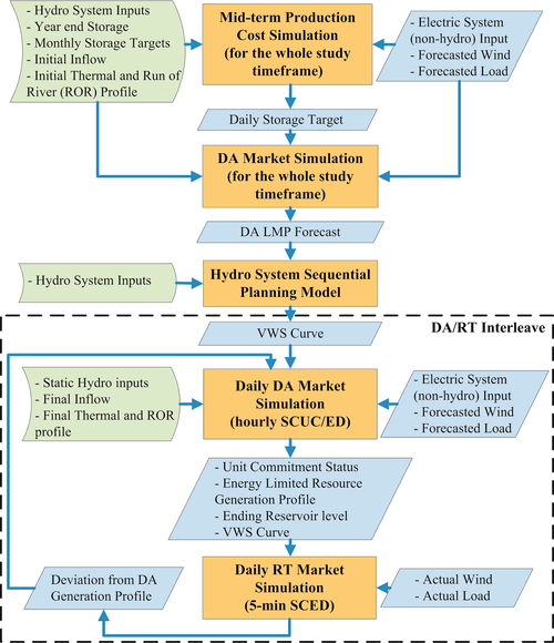
The process starts with taking long-term hydro-storage constraints and decomposing them into daily storage constraints using a mid-term (MT) schedule model. Based on the initial storage level, expected year-end storage level, run-of-river (ROR) profiles, and monthly storage targets, the MT schedule model simulates the long-term system operations using load-duration curves and produces short-term storage constraints for the daily modeling.
The first iteration of DA market simulation is then performed for a whole year to generate the forecasted hourly DA LMPs for the year. In DA market simulation, the forecasted wind and load profiles are used.
With the LMP forecast, a separate tool named hydro-system sequential-planning model is then used to create the VWS curve for the market simulation.
The final market simulation consists of interleaving the DA market with the RT market to simulate near actual market operations similar to how the MISO market operates. The hydro’s generation in the RT market follows the DA schedule, but is allowed to deviate from the DA schedule based on price differences between the RT and DA markets. The differences in the amount of water used in the RT market and that projected to be used by the DA market will be taken into account during the next simulation day using the VWS curve.
5.3 Simulation Subtasks
5.3.1 Use MT schedule model to generate daily storage target
The first step of the simulation process is to convert the monthly water-storage targets to daily storage targets. The monthly water storage targets are decomposed by running a simplified non-chronologic simulation in which the hourly chronological load profile for each month is simplified as a load-duration curve. In the simplified non-chronologic simulation, instead of optimizing the total production cost on a daily interval like the DA market does, the total system production cost for each month is optimized. Inter-temporal constraints such as ramp-up/ramp-down rates and minimum run/down time are ignored in the simplified non-chronologic simulation. By using duration curves rather than a chronological simulation to simplify the temporal constraints, the MT model considers the monthly water-storage targets on dispatchable hydro units and still simulates at a time step of an hour. As the result of the MT simulation, the hourly hydro-unit output can be obtained, which is used to calculate the daily ending storage volume by back calculating the water usage for each day. The daily ending storage volume is used as the preliminary hydro-system hourly dispatch schedules for the first round of DA simulation.
5.3.2 Run DA model to generate DA-LMP forecast
After the daily storage target is obtained using the MT model, the daily storage target is passed to the DA model. Then the DA model is executed to generate the hourly LMP forecast for the whole year. In this round of the DA simulation, for each hydro-storage unit, the daily maximum available energy is considered based on MT simulation results. Then an hourly simulation is performed that determines the optimal generation dispatch for each hour.
5.3.3 Use hydro-system sequential-planning model to create VWS curve
The hydro-system sequential-planning model takes an hourly LMP forecast as an input and considers detailed hydro-system operating characteristics. The hydro-system sequential-planning model determines the generation schedules of hydro-storage units under multiple possible hydraulic conditions. This information is then used to create a VWS curve.
The general mathematical model of the hydro-system sequential-planning tool is:
![]()
Subject to:
where C is the cost, ep is the export amount of MH, im is the import amount of MH, λ is the LMP, sv is the storage volume in the water reservoir, wfin is the water inflow, wftail is the tail flow, w is the hourly hydro-unit water usage, and ws is the amount of water that gets spilled.
Equation (1) balances the supply and demand of the MH system. Equations (2) and (3) price the export revenue and import cost, respectively. Equation (4) updates the water-storage volume in each storage reservoir. Equation (5) defines the tail flow for each hydro unit. The water-storage volume constraints for each reservoir are enforced in function (6).
6 DA/RT Interleave Method
Most long-term production-cost simulation tools simulate the hourly operations of the system (DA market) for the whole simulation timeframe without considering the interactions between the hourly simulation and sub-hourly simulation (if that function is available) [19–21]. In the real system, however, it is important for generation companies (Gencos) to evaluate the RT-settlement results from the previous day in order to prepare the next DA bids. This need is especially critical for energy-limited resources such as hydro units as the DA/RT dispatch difference will change the available energy for those units, which affects the DA dispatch for the next day. For example, if only the DA simulation is considered, the simulation model will generate the operating schedule of hydro-storage units for the whole simulation horizon. If the RT market is also considered, however, the hydro-storage units’ generation might be different from the dispatch results in DA. For example, if hydro-storage units participate actively in the RT market and keep generating more in the RT market, they will eventually use up the water reservoir prematurely. A DA-only or RT-only simulation model cannot capture that scenario. Figure 7.4 shows the existing methods for DA and RT market simulations. Most of the software tools perform long-term DA-only simulation (the upper box) [22]. Some tools can perform long-term RT-only simulation (the lower box). A few tools can perform DA simulation for the whole simulation timeframe and then conduct RT simulation [6].

In this study, a novel simulation method named Interleave method is proposed. To the best of our knowledge, it is the first time that this approach is proposed and applied on a large electric system. The simulation process of the Interleave method is demonstrated in Figure 7.5. Both the long-term DA market simulation and the RT market simulation are broken into daily simulation problems. After each daily DA simulation, the unit-commitment and economic-dispatch decisions are passed to the hydro-storage model and the RT problem. Based on the DA results, the hydro-storage model adjusts the hydro units’ bids in the RT problem. Then the RT problem conducts a 5-minute simulation for the same day. After the RT problem is finished, the hydro-storage model is updated again using the RT economic dispatch results. This process is repeated throughout the simulation horizon.

In the DA and RT market simulations, the energy and ancillary services markets are co-optimized. Three types of ancillary services are considered in the simulation: regulation up, regulation down, and contingency reserve. In the co-optimization problem, the sum of energy commitments and reserve commitments respect reservoir limits.
6.1 Run DA Model to Simulate DA Market Operation
The process of using the VWS curve to determine DA hydro-energy bids is illustrated in Figure 7.6. V1 and P1 are the water-storage volume and corresponding value of water at the beginning of the DA market simulation, respectively.
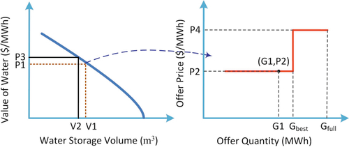
A hydro unit’s DA market offer curve is determined by hydro-unit efficiency curve and the marginal value of water. The hydro unit’s efficiency curve can be derived by taking the derivatives of the hydro-unit performance curve. A hydro-unit offer curve is shown on the right side of Figure 7.6.
The two segments of the offer curve correspond to the first two segments of the hydro-unit performance curve. Gbest and Gfull are the best-gate and full-gate generation capacities, respectively. The value of one cubic meter of water can be calculated by dividing P1, which is the value of water in $/MWh, by the average hydro-unit efficiency (in MWh/m3). P2 and P4 are calculated by multiplying the value of one cubic meter of water with the generation efficiencies (in MWh/m3) of the first generator and the second generator, respectively, as shown in equations (8) and (9).

where ηdh1 and ηdh2 are generation efficiencies of the first generator and second generator, respectively.
Note that the third generator represents the effect of a spill, which means the storage reservoir is full and the value of water is zero. This will create an offer price of zero for the offer curve.
Based on the ROR profiles, forecasted wind and load profiles, electric system inputs, and hydro-energy DA market bids, the DA model conducts hourly SCUC and SCED for the next day. As the result of DA market simulation, the hydro energy’s bids are settled. The accepted offer quantity for each hour is denoted as G1 in Figure 7.6. The total hydro-storage unit water consumption during the day can be obtained by summing up the hourly accepted offer quantity G1 for the 24 hours. After the DA-market simulation, the water-storage volume after the DA market can be updated using equation (10).

where V2 is the water-storage volume in the reservoir after the DA market simulation, and W is a water-usage function that calculates the amount of water used to generate a specific amount of energy.
6.2 Run RT Model to Simulate RT-Market Operation
In the RT market, the simulation engine only has access to the current 5-minute period of the system status and is unable to know if a unit should generate now or wait for better opportunities in the future. Because of this, the hydro units’ dispatch information needs to be passed from the DA simulation to the RT simulation. The DA simulation optimizes the hourly system operations using forecasted wind and load profiles, while the RT simulation looks at the 5-minute level that has actual wind and load information in it. This implies the simulation needs to be flexible in order to balance the value gained by following the DA dispatch and the value from over- or under-generating to take advantage of DA/RT system condition changes.
A unique bidding method called tiered bidding is proposed to make sure hydro energy’s RT-generation output generally follows the DA schedule, but also can deviate from DA dispatch based on RT LMPs. Figure 7.7 illustrates the process of using the VWS curve and the updated water-storage volume to create the tiered bids in the RT market. First, the updated value of water (P3) is obtained based on the VWS curve and the current water-storage volume. Then based on P3 and G1, a group of RT offers can be obtained as shown in Figure 7.7. The RT bidding curve is a step function. For each bid segment, the offer price and offer quantity are determined by multiplying P3 with a value of water multiplier and multiplying G1 with an offer-quantity multiplier, respectively. For example, the value of the water multiplier and offer quantity multiplier of the 4th segment are 0.6 and 0.8, respectively. So the 4th offer segment in the offer curve is the line between (0.8G1, 0.6P3) and (G1, 0.6P3).
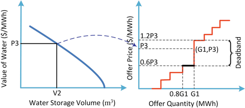
As illustrated in Figure 7.7, the RT offer curve is obtained by multiplying P3 with various offer-price multipliers and multiplying G1 with various offer-quantity multipliers. Each hydro unit submits the same set of offer prices for the 24 hours (the offer quantities at each hour are based on the cleared quantity for the same hour in the DA simulation). In order to make sure the RT generation does not deviate from the DA schedule when the LMP difference is small, the RT offers are set up in such a way that RT dispatch will be the same as the DA dispatch if the RT market LMP is with a certain range of the value of water. This range is called deadband. The size of the deadband and the values of offer-price multipliers determine how sensitive the hydro-storage unit is to the RT-market LMP fluctuations.
6.3 Wind/Load Profiles
Wind units are modeled as a dispatchable intermittent resource (DIR), which means wind units can actively bid in the energy market and can be dispatched down when needed (instead of being curtailed manually by operators) [23]. DIR is not eligible to supply operating reserves. In our formulation, the DA problems consider the forecasted wind output for the next day and make commitment/dispatch decisions accordingly. In this way, instead of being modeled as negative load as many previous studies do [24,25], wind can be dispatched up or down based on market conditions and forecasted maximal wind output [26].
Creating the 5-minute wind/load profile for the RT simulation is a 3-step process:
Based on 2008–2011 MISO historical wind/load hourly and 5-minute data, calculate a) statistics of the differences between the forecasted DA hourly MW outputs and the actual hourly MW outputs, and b) statistics of the differences between the actual 5-minute values and the actual hourly values. In this way, the mean and variance of the DA hourly wind/load forecast errors and RT wind/load intra-hour fluctuations are obtained, as illustrated in Table 7.1. The statistics are compiled using aggregate MISO forecasts/actuals and as such some of the variation in wind may have been reduced due to geodiversityIncreased variation in the model is considered by using separate wind forecasts for every wind site and doing a separate statistical draw on each wind site independent of the other wind sites.
Table 7.1
Wind and Load Data Statistics
| Wind Variance | Load Variance | |||
| Statistics | (DA Forecast - Hourly Actual)/Hourly Actual | (5-min Actual - Hourly Actual)/Hourly Actual | (DA Forecast - Hourly Actual)/Hourly Actual | (5-min Actual - Hourly Actual)/Hourly Actual |
| Mean | 13.08% | 0.03% | 0.35% | 0.01% |
| Std Dev | 39.89% | 2.42% | 1.89% | 1.20% |
| Max | 308.65% | 108.93% | 14.15% | 56.48% |
| Min | −96.50% | −46.40% | −17.03% | −38.54% |

Based on the mean and variance of the DA hourly wind/load forecast errors, the hourly variance can be applied to the hourly DA forecast to create the RT hour ending value. In this study, for each wind farm, there is a unique nominal 1-MW multi-variate wind power hourly production time series to represent the DA forecast. This hourly wind forecast is obtained from the Eastern Wind Dataset created by AWS-Truewind and National Renewable Energy Laboratory (NREL) [27].
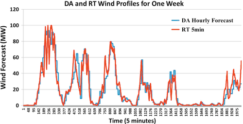
The wind/load intra-hour statistical information can be applied to create the RT 5-minute value. The DA hourly wind forecast and the corresponding RT 5-minute profile are shown in Figure 7.8, for one wind farm.
7 Implementation
Because of the intricacies in modeling a hydro-storage system and its effect on wind variability and ancillary service prices, production-cost software called PLEXOS was chosen as the primary simulation tool for this study. PLEXOS is a power-market simulation tool that uses mathematical programming and stochastic optimization techniques to provide an analytical framework for power-market modelers [28]. The users can select among multiple commercial optimization solvers, such as CPLEX, to solve the optimization problem. The simulation model can simulate the wholesale electricity market in a similar way as many ISO/RTO market applications do, but with a much longer simulation timeframe [29–31].
The interleave method is implemented by adding custom .NET assemblies (libraries) into the PLEXOS database and having the PLEXOS engine execute the assemblies at runtime.
7.1 Simulation Results
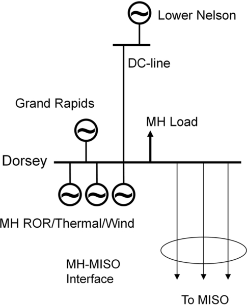
The proposed simulation methodology is used to evaluate the economic benefits of expanding MH’s participation in the MISO RT market. The MH hydro system is set up as a group of 13 ROR hydro units and 2 dispatchable hydro units. As shown in Figure 7.9, the MH system is modeled as two buses linked by a DC line. Thirteen ROR hydro units are modeled with MW schedules provided by MH to match the water-condition assumptions. The power capacities of the two MH dispatchable hydro units, Grand Rapids and Lower Nelson, are 465 MW and 3518 MW, respectively. The detailed Manitoba Hydro model is linked with the rest of the Eastern Interconnection model (excluding Florida, ISO New England, and Eastern Canada). The MISO-MH interface consists of three AC-lines between MH and MISO. The rating from MH to MISO is 1850 MW, while the rating from MISO to MH is 850 MW.
The proposed simulation methodology is applied to the whole Eastern Interconnection system, which has about 5800 generators, 70000 buses, and 90000 branches. About 1100 contingencies are considered in the security-constrained unit-commitment and economic-dispatch models. Most of the contingencies are (n-1) contingencies, but there are also some (n-2) contingencies. Under each contingency, the flows on one or more related transmission lines or transformers are monitored and their flow limits are enforced. The contingencies are represented as additional flow constraints in the security-constrained unit commitment and economic-dispatch models, as shown in function (11).

where f is the flow limit, P is generator output, Li is the i-th transmission line, Gj is the j-th generator, SFmGjLi is the shift factor of generator Gj on transmission line Li under the m-th (n-k) contingency, and NG is the total number of generators.
In our study, out of the 5800 generators considered in the simulation, 532 generators are hydro units. The 13 ROR units and 2 dispatchable hydro units in the MH system are modeled in detail based on the information provided by MH, e.g., hourly ROR profiles. The other 517 hydro units are modeled as energy-limited resources that have monthly energy limits. The simulation time is about 120 hours for the 12-month simulation using a personal computer (PC) running Windows 7 with 3.07GHz dual-core CPU and 128GB of RAM.
MH participates in MISO’s market through the use of two market resources called External Asynchronous Resource (EAR) and E-tag. MH is not within MISO’s market footprint and is its own balancing authority, so the generation and transmission systems in MH are not modeled in MISO’s market application. In the MISO market, the whole MH system is considered as an EAR and can provide energy, regulation, and contingency reserves to MISO. From MISO’s perspective, an EAR can be considered as an asynchronous DC tie between MISO and an asynchronous island where the system generation-load balancing is performed independent of MISO. In the DA and RT markets, MH submits price-MW offers through the EAR, and MISO makes economic-dispatch decisions on the MH offers. MH can also submit an E-tag to arrange a fixed interchange schedule.
Figure 7.10 shows the MH-MISO interface flows and the storage volumes of MH dispatchable hydro units during one week.
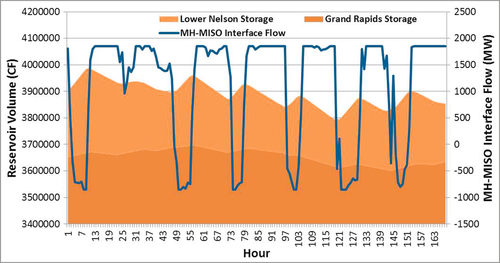
When MH-MISO interface flows are positive, MH sells electricity to MISO so the total storage volume decreases. When MH-MISO interface flows are negative, MH purchases electricity from MISO to substitute the generation of its dispatchable hydro units. As the result of that, the total storage volume increases, which has the same effect as pumping.
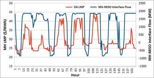
Figure 7.11 shows the MH-MISO interface flows and MH DA LMPs during one week. As shown in Figure 7.11, there is a strong correlation between MH DA LMPs and MH-MISO interface flows. When the MH DA LMPs are high, MH exports to MISO to earn economic benefits; when the MH DA LMPs are low, MH imports from MISO to supply its own load. The MISO to MH flows constantly hit the interface flow limit at 1850 MW, which indicates potential economic opportunity for investing new transmission lines between MH and MISO.
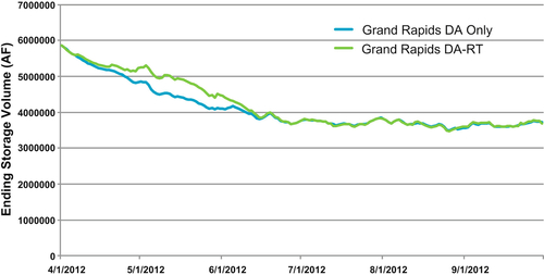
Compared with DA market-only simulation, the DA/RT interleaved simulation can capture the over- or under-usage of water in the RT market. Figure 7.12 shows the storage volume of Grand Rapids over a six-month horizon under two simulations: DA-only simulation and DA-RT-interleaved simulation. The difference between the storage-volume curves demonstrates the effect of RT simulation on the actual storage volume. In this example, it was more profitable for MH to hold back in the RT market and sell less than scheduled in the DA market in order to use the water later.
The current EAR is one-directional as it only allows MH to sell to MISO. In the RT market, if MH wants to buy from MISO, it needs to submit an “E-tag,” which means submitting a fixed interchange schedule. This fixed interchange schedule is a price-taker. It is possible that while a fixed interchange is submitted through E-tag trying to take advantage of the low DA prices, the RT market prices turn out to be much higher than the DA prices, which drastically increase MH’s purchase payment. As a result of the high financial risks associated with the E-tags, MH is very conservative in RT-market participation. The RT tiered-bidding curve under the current one-directional EAR is shown in Figure 7.13.
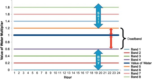
The deadband of the RT tiered-bidding curve is between 60% of the value of water and 120% of the value of water. The uneven deadband above and below the value of water represents MH’s limited participation in MISO’s RT market. The bands above the value of water represent the EAR, while the bands below the value of water represent the E-tag. As MH has to use E-tag to schedule RT fixed interchange (purchase), which exposes MH to high financial risks. MH will only schedule purchases when there is a high price difference between the RT price and the value of water. So there is a high gap between band 5 and the value of water. The value of the deadband is determined by the experts from MH based on their practical experience concerning the way MH bids into MISO’s market.
One of the goals of the Manitoba Hydro Wind Synergy Study is to evaluate the potential economic benefits of enabling MH’s bi-directional RT market participation through expended EAR. With the bi-directional EAR product, MH can submit energy purchase offers (i.e., negative MW/price curve) through the EAR and the MISO market applications will clear the negative generation offers to minimize total MISO production cost. The bi-directional EAR enables MH to buy with certainty in the RT market as there is less financial risk for MH to use EAR than energy E-tags. The RT tiered-bidding curve under extended EAR is illustrated in Figure 7.14. Compared with the bidding curve shown in Figure 7.13, the extended EAR RT tiered-bidding curve enables MH to respond to RT price fluctuations more aggressively.
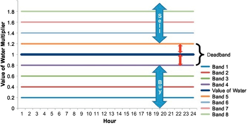
Figure 7.15 shows the RT LMPs for one day under one-directional EAR and under bi-directional EAR

Under the extended EAR, the deadband is smaller, which enables the dispatchable hydro units to respond to RT LMP changes more aggressively. As shown in Figure 7.15, when RT LMPs drop, the extended EAR allows dispatchable hydro units to adjust their generation when the RT LMPs hit 0.8VWS. Under one-directional EAR, however, dispatchable hydro units can not adjust their generation until the RT LMPs hit 0.6VWs.
Increased MH RT market participation helps to reduce MISO RT price volatility and ultimately system production cost by allowing MH to respond to unforeseen system fluctuations in MISO. Figures 7.16 and 7.17 show the monthly MISO production-cost savings and operating-reserve (both regulation and contingency) savings, respectively.
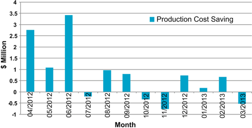

As shown in Figure 7.16 and Figure 7.17, the overall benefits are positive for both production-cost and reserve-cost savings throughout the year, but some months experience negative savings because of changing water usage between the simulations, which shifts benefits on either side of the monthly border. Energy benefits are also higher in the Spring since MH has more water to trade within the market.
Compared with the status quo case (i.e., with the unidirectional EAR), the bi-directional EAR case can achieve $8.74 million in MISO annual production-cost savings and $0.1 million in MISO annual-reserve cost savings. Additionally, by extending the RT-market participation, the total wind curtailment in MISO is reduced by 21 GWh, which is about 0.05% of the total potential wind energy. Note that this is only the benefit achieved by converting the one-directional EAR to the bi-directional EAR.
8 Conclusions
This chapter proposed a detailed DA and RT markets simulation methodology, which includes a detailed hydro-storage system model. Hydro-storage systems have more complexity than is present in other generation resources. With the help of the MH planning and operations departments, the operating characteristics as well as DA/RT market participation strategy of two hydro-storage units were modeled in great detail. A hydro unit’s performance curve was represented as three generators and their associated constraints in the simulation model. The tiered-bidding method was combined with the value of water in the storage curve to represent the hydro-storage units’ bidding curves in the RT market. A novel simulation method called the Interleave method was implemented to enable hydro units to adjust their bids at the beginning of each daily DA and RT market simulation based on the VWS curve and water-storage volume.
The proposed simulation methodology is employed in the Manitoba Hydro Wind Synergy Study to evaluate the potential economic benefits of extending MH’s participation in MISO’s RT market through the implementation of an extended EAR product. The simulation shows that, by extending the market participation in MISO’s energy and ancillary services markets, MH benefits from increased energy/reserve payments, while MISO benefits from more efficient dispatch, reduced reserve costs, and less wind curtailment.
Besides the application illustrated in the case-study section, the proposed simulation methodology can also be used to perform many other kinds of economic studies, such as evaluating new generation or transmission facilities investments or accessing market rule changes.
Appendix
The procedures to get the final VWS curve are:
The MH-only system is simulated for a year at different starting volumes for a reservoir. The hydro-system sequential-planning tool (described in Section 6)) is used to maximize the profit of the whole hydro system by determining the optimal-dispatch schedule for the dispatchable hydro units. The profits of MH at different starting volumes can be calculated in this step.
Calculate the incremental value of water (IVW) at different starting volumes. The incremental value of water (in $/Mwh) between two starting volumes x1 and x2 can be calculated by function (12) below. Multiple values of water points are created in this process.
where R is the total amount of revenue for the whole simulation horizon with a certain starting storage volume, and ηdh is the average hydro-turbine efficiency in MWh/m3.
The average hydro-turbine efficiency is obtained from historical data by dividing the total historical generation output over a long period of time by the total water inflow during that time frame.
Repeat steps 1-2 for several different hydrologic scenarios to get the incremental value of water at different starting volumes for each water-inflow scenario.
Average the incremental values of water calculated in step 3 under all different hydrologic scenarios using their probabilities to create the final VWS curve. Three hydrologic scenarios, low-water scenario, medium-water scenario, and high-water scenario, are considered in this study, with probabilities 20%, 60%, and 20%, respectively.