
Operation of Independent Large-Scale Battery-Storage Systems in Energy and Reserve Markets*
Hossein Akhavan-Hejazi; Hamed Mohsenian-Rad Electrical Engineering Department at the University of California, Riverside, CA, USA.
*
This work was supported by NSF Grant ECCS 1253516.
Abstract
In this chapter, we consider a scenario where a group of investor-owned independently-operated storage units seek to offer energy and reserve in the day-ahead market and energy in the hour-ahead market. We are particularly interested in the case where a significant portion of the power generated in the grid is from wind and other intermittent renewable energy resources. In this regard, we formulate a stochastic programming framework to choose optimal energy and reserve bids for the storage units that takes into account the fluctuating nature of the market prices due to the randomness in the renewable power generation availability. We show that the formulated stochastic program can be converted to a convex optimization problem to be solved efficiently. Our simulation results also show that our design can assure profitability of the private investment on storage units. We also investigate the impact of various design parameters, such as the size and location of the storage unit on increasing the profit.
Nomenclature
h, t Indices for hours.
k Index of random wind-generation scenarios.
K Total number of random wind-generation scenarios
γ The weight/probability for different scenarios.
![]() Expected value operator.
Expected value operator.
P Storage bid in the day-ahead market for power.
R Storage bid in the day-ahead market for reserve.
p Storage bid in the hour-ahead market for power.
r Actual utilization of the storage reserve.
rmax The upper bound for reserve utilization.
CP Price value for energy in the day-ahead market.
CR Price for reserve in the day-ahead market.
cp Price for energy in the hour-ahead market.
cr Price for reserve utilization in the hour-ahead market.
Clinit Initial charging level of the battery unit.
Clfull Maximum charging capacity of the battery unit.
Clmin Minimum charging capacity of the battery unit.
![]() The total number of peak price hours.
The total number of peak price hours.
hj* The jth hour from the set of peak price hours.
1 Introduction
Due to their intermittency and inter-temporal variations, the integration of renewable energy sources is very challenging [1]. A recent study in [2] has shown that significant wind-power curtailment may become inevitable if more renewable power-generation resources are installed without improving the existing infrastructure or using energy storage. other studies, e.g., in [3–5] have similarly suggested that energy storage can potentially help integrating renewable, in particular wind, energy resources. Although this basic idea has been widely speculated in the smart-grid community, it is still not clear how we can encourage major investment for building large-scale independently-owned storage units and how we should utilize the many different opportunities existing for these units. Addressing these open problems is the focus of this chapter.
The existing literature on integrating energy storage into smart grids is diverse. One thread of research, e.g., in [6–8], seeks to achieve various social objectives such as increasing the power-system reliability, reducing carbon emissions, and minimizing the total power-generation cost. They do not see the storage units as independent entities and rather assume that the operation of energy-storage systems is governed by a centralized controller. As a result, they do not address the profitability of investment in the storage sector and the possibility for storage units to participate in the wholesale market. Another thread of research, e.g., in [9–12], seeks to optimally operate a storage unit when it is combined and co-located with a wind farm. They essentially assume that it is the owner of the wind farm that must pay for the storage units. Clearly, this assumption may not always hold and it can certainly limit the opportunities to attract investors to build new energy-storage systems. Finally, there are some papers, such as [12–16], that aim to select optimal strategies for certain storage technologies, e.g., pumped hydro-storage units, to bid in the electricity market. However, they typically do not account for the uncertainties in the market prices, which can be a major decision factor if the amount of renewable power generation is significant. Moreover, they do not consider the opportunities for the energy-storage systems to participate not only in energy markets but also in reserve markets. Finally, the operation of large storage units such as pumped hydro are different from that of limited energy-storage units, which are of interest in this work. While pumped hydro units are mostly limited to the discharge rate or the capacity of turbines, batteries are limited by the available state of charge.
Therefore, the following question is yet to be answered: How can an energy-storage unit that is owned and operated by a private investor bid in both energy and reserve markets to maximize its profit, when there exists a significant penetration of unpredictable resources in the power grid? The storage unit may or may not be collocated with renewable or traditional generators. In fact, the location and size of the unit is decided by investors based on factors such as land availability and spot-price profile. In order to optimally operate the storage unit of interest, we propose a stochastic optimization approach to bid for energy and reserve in the day-ahead (DA) market and energy in the hour-ahead (HA) markets. Here, we assume a reserve-market structure similar to a simplified version of the day-ahead scheduling reserve market in the PJM (Pennsylvania, New Jersey, Maryland) inter-connection [17], where the exact utilization of the reserve bids is not decided by the storage unit; instead, it is decided by the market. As a result, finding the optimal charge and discharge schedules is particularly challenging when the storage unit participates in the reserve market. Another challenge is to formulate the bidding-optimization problem as a convex program to make it tractable and appropriate for practical scenarios. Compared to an earlier conference version of this work in [18], in this chapter, a more accurate solution approach is proposed to solve the formulated non-convex optimization problems. The new solution is more general and allows selling unused reserves in the hour-ahead energy market. Our contributions in this chapter can be summarized as follows:
• We propose a new stochastic optimization bidding mechanism for independent storage units in the DA and HA energy and reserve markets. Our design operates the charge and discharge cycles for the batteries such to assure meeting the future reserve commitments under different scenarios, regardless of the uncertainties that are present in the decision-making process.
• An important feature in our proposed market-participation model is that the power grid does not treat independent storage units any different from other energy and reserve resources. Therefore, our design can be used to encourage large-scale integration of energy-storage resources without the need for restructuring the market.
• We show through computer simulations that our proposed optimal energy and reserve-bidding mechanism is highly beneficial to independent storage units as it assures the profit gain of their investment. We also investigate the impact of various design parameters, such as the size and location of the storage unit on increasing the profit.
The rest of this chapter is organized as follows. The system model and the optimal-bidding problem formulation are explained in Section 2. Two different tractable design approaches to solve the formulated problems are presented in Section 3. Simulation results are presented in Section 4. The concluding remarks and future work are discussed in Section 5.
2 Problem Formulation
Consider a power grid with several traditional and renewable power generators as well as multiple independent energy-storage systems. We assume that not only the generators but also the storage units can bid and participate in the deregulated electricity market. As pointed out in Section 1, our key assumption is that the storage units are not treated any differently than other generators that participate in the energy or reserve markets. Since the energy-storage units in the system are owned and operated by private entities, they naturally seek to maximize their own profit. The stochastic wind generation, however, may create some extra benefits for storage units, considering that energy and reserve market prices may fluctuate significantly, giving them more opportunities to gain profit in the presence of high wind-power penetration. The assumption of high wind-power penetration adds to the load-forecast error component of the operating (DA scheduling) reserve,1 since the wind generation is typically considered as part of the net load.
With more fluctuations in the net load, the operating reserves are more likely to be called up frequently. We also assume that the storage unit operates as a price-taker, i.e., it operates as a self-scheduling (must-run) unit and does not bid for price. Therefore, the storage unit will be compensated based on market-clearing prices. Of course, at the time of bidding in the day-ahead market, the storage unit does not know the actual prices, rather it only has an estimate of them. We also assume that the storage unit’s operation does not have impact on market prices due to its typically lower size (in megawatts) compared to traditional generators.
The main decision variables of the storage unit in our system model are the energy and reserve quantities for different hours in the DA market. However, the storage decisions and operation in the day-ahead market and hour-ahead (real-time) market are highly tied together. The storage unit’s bid in the DA market has a direct impact on the storage unit’s future profit in the HA market, since the commitments in the DA market will put some constraints in the charging and discharging profiles of the storage unit. An example of the charging and discharging cycles in the DA energy and reserve markets is shown in Figure 11.1, where the storage unit has committed to offer energy and reserve at three hours: h1 = 7:00 AM, h2 = 3:00 PM, and h3 = 8:00 PM. In each case, the state-of-charge (SOC) of batteries must reach a level Clh ≥ Ph + Rh for all h ∈ {h1, h2, h3}.

When a storage unit bids for reserve at a particular hour of the DA market, all, part of, or none of its committed reserve could be used. This will create uncertainty in the charging level of the storage unit; and depending on which value presumed for the utilization of reserve, the storage might have more or less charge available in real time. Therefore, even for the DA market bidding, the storage unit should have some information on the hour-ahead operation model.
When an independent storage unit submits a bid to the day-ahead market (DAM), it seeks to maximize its profit in the DA market plus the expected value of its profit in the next 24 hour-ahead markets (HAM). Therefore, prior to submitting the bids into the DA market, the storage unit should solve an operation-optimization problem in both the DA and HA markets for all the services that it aims to provide. The services that we aim to consider in this chapter are: DA power, DA reserve, and HA power.2 Also the storage needs some estimation of the prices at hours h = 1 – 24 in both DA and HA markets. The prices of the HA markets on the next day will have more uncertainty due to availability variation and uncertainty in wind generation. The decision-making process of storage and the input information required is illustrated in Figure 11.2 This can be mathematically formulated as the following optimization problem3:


Note that P can take both positive and negative values while R is always positive. Negative values for P indicate purchasing power, i.e., charging. The expected value of the profit in the HA market, i.e., the second term in the objective function in (1), depends on not only the choices of P and R, but also the storage unit’s decision on the amount of power to be sold in the HA market ph, the price of power in the HA market c![]() , the price of reserve in the HA market c
, the price of reserve in the HA market c![]() , the actual reserve utilization in the HA market
, the actual reserve utilization in the HA market ![]() and the fluctuations in wind generated. The third constraint assures that the reserve bid is non-negative. Note that, at the time of solving (1),
and the fluctuations in wind generated. The third constraint assures that the reserve bid is non-negative. Note that, at the time of solving (1), ![]() are unknown stochastic parameters.
are unknown stochastic parameters.
Using the definition of mathematical expectation, we can rewrite the second term in (1) as a weighted summation of the aggregate HA profit terms, denoted by HAM, at many but finite scenarios, where the weight for each scenario is the probability for that scenario. That is, we can write:

where HAMk denotes the aggregate HA profit when scenario k occurs. We have ∑ k = 1Kγk = 1. It is worth clarifying that one of the main causes for profit uncertainty is the fluctuations in available wind power. Therefore, in our system model, each scenario is derived as a realization of available wind power at different wind-generation locations, given the wind-speed probability distribution functions, which is assumed to be available, e.g., by using the wind-forecasting techniques in [19–21]. For each scenario k, the corresponding aggregate HA profit can be calculated as follows:

where pk is the adjustment to the power draw or power injection of the storage unit in the HA market for h = 1,…, 24, under scenario k. Here, cpk, crk, and rk are the actual realizations of the stochastic parameters ![]() when scenario k occurs. We note that they are all set by the grid operator. The constraint in (3) indicates that the total generation bid up to hour h of the HA market has to be limited to the total charge available to the storage unit at hour h. Such total charge is calculated as the initial charge minus the sum of all the power drawn from the storage including the bid for power, i.e., Ph, and the reserve utilization in the HA market, i.e., rk,h, for all previous hours t = 1,…, h – 1.
when scenario k occurs. We note that they are all set by the grid operator. The constraint in (3) indicates that the total generation bid up to hour h of the HA market has to be limited to the total charge available to the storage unit at hour h. Such total charge is calculated as the initial charge minus the sum of all the power drawn from the storage including the bid for power, i.e., Ph, and the reserve utilization in the HA market, i.e., rk,h, for all previous hours t = 1,…, h – 1.
Note that the actual reserve utilization rk,h may not always be as high as the committed reserve, as the grid may not need to utilize the entire reserve power offered by the storage unit. As a result, in the HA market, the storage unit needs to make corrective decisions to make the best use of any extra charge that is available due to different reserve utilizations caused by different wind availability and load scenarios. This makes dealing with parameter rk,h particularly complicated, as shown in Figure 11.3. Let rh,kmax denote the maximum reserve power that the grid operator will need from the storage unit of interest at hour h if scenario k occurs. It is required that:

On the other hand, parameter rk,h also depends on the storage unit’s reserve commitment for each hour h based on its bid in the DA market. Therefore, it is further required that
From (4) and (5), at each hour h and scenario k, we have:
Replacing (6) in the HA problem (3), it becomes:

Next, we use the following equality [22]:
and combine problems (1) and (3) into a single problem:

However, optimization problem (9) is non-convex and hence difficult to solve. Note that the non-convexity is due to the way that the min function has appeared in the first constraint.
3 Solution Methods
In this section, we consider some practical assumptions in order to make problem (9) more tractable. In this regard, we take two approaches for choosing pk,h before solving the rest of the optimization problem. In both cases, we assume that the participation of the storage unit in the HA market is mainly to sell the unused charge from reserve bids. Therefore, for both approaches we always have pk,h ≥ 0.
3.1 The First Approach
In this approach, the intuition is that the storage unit immediately sells any excessive power available at each hour in case the entire committed reversed power is not utilized. That is, at each hour h and for each scenario k, we choose:
The second term in the objective in problem (9) becomes:
Next, we note that based on (10), the total power sold in the HA market at hour h is:

Therefore, the first constraint in problem (9) becomes:
The second constraint can also be revised as:
From (9), (11), (13), and (14), we can rewrite problem (9) based on (10) and with respect to the rest of the variables as:

Since min is a convex function and the rest of the objective function and constraints are all linear, problem (15) is a convex program, as long as crk,h – cpk,h ≥ 0, for all k = 1,…, K and for all h = 1,…, 24. Interestingly, this condition holds in most practical markets, where the reserve-utilization price is relatively higher than the energy-clearing price. Therefore, we maintain this assumption for the rest of this chapter. If this condition holds, then optimization problem (11) can further be written as a linear program. To show how, next, we introduce an auxiliary variable
υk,h and rewrite problem (15) as:

where v is a 24 K × 1 vector of all auxiliary variables. It is easy to show that at optimality, for all k = 1,…, K and any h = 1,…, 24, we have. υk, h = min{rk,hmax, Rh}. Therefore, while problems (15) and (16) are not exactly the same, they are equivalent, i.e., they both lead to the same optimal solutions [22, Chapter 4]. As a result, solving one problem readily gives the solution for the other problem. Linear program (16) can be solved efficiently using the interior point method [22].
3.2 The Second Approach
In this approach, instead of immediately selling the excessive power Rh – rk,h at hour h, we may wait and sell accumulated unused reserve powers in an HA market with high price of electricity. We define an hour h* as a “peak hour” if no other hour h > h* exist with a cpk,h > cpk,h*, i.e. a higher price for energy. Based on the second approach, for each k = 1,…, K and h = 2,…, 24, we select pk,h as follows:
• If h is not a peak hour then pk,h = 0.
• If h is the jth peak hour, j = 1,…, ![]() , then:
, then:

At each peak hour, the amount of electricity sold is equal to the total unused reserve since the previous peak-hour. Next, we replace pk,h in (9) with selling strategy explained above. The second term in the objective function in problem (9) becomes:

where
Next, we note that from (17), we have:
and
Therefore, a sufficient condition for the first constraint in (9) to hold is to satisfy the following more restrictive constraint:
Next, consider the second constraint in (9). Given the complexity of this constraint, we need to separately analyze two different cases. On one hand, for each peak hour hj*, we have:

By replacing (23) in the second constraint in (9) it becomes:

On the other hand, at each non-peak hour h = hj* + 1, …, hj*+ 1 − 1, since no power is sold in the HA market, we only need that the sum of the DA power bids and the actual reserve utilization do not exceed the maximum charge level permitted for the batteries. The second constraint in (9) for each non-peak hour h ∈ {hj* + 1, …, hj*+ 1 − 1} become:
From (9), (18), (22), (24), and (25) and after using the auxiliary variable vector v, we propose to solve the following optimization problem as our second approach:
Unlike problem (9), problem (26) is a convex program. Therefore, problem (26) is significantly more tractable as it can be solved using standard convex-optimization techniques, e.g., see [22]. However, in general, solving problem (26) gives a sub-optimal (not necessarily optimal) solution for the original optimization problem (9) for the following two reasons. First, the first constraint in (26) is more restrictive than the first constraint in (9). This can limit the feasible set. Second, there is no guarantee for problem (26) that at its optimality we have υk, h = min{rk,hmax, Rh}. Therefore, it is possible that the optimal solution of problem (26) does not satisfy the second constraint in problem (9). In such rare cases, in order to maintain a feasible solution, the storage unit needs to sell any excessive stored energy into the HA energy market, even if the next hour is not a peak-price hour. This corrective action can cause some minor sub-optimality. Nevertheless, we will see in our simulation results that the optimality gap of our second approach is very minor.
3.3 Selecting Stochastic Price Parameters
Before we end this section, we note that in order to solve problems (16) and (26), we must know the values of rk,hmax, cpk,h, and crk,h as well as CPh and CRh. These parameters are obtained in an off-line calculation by solving a standard stochastic unit commitment (SUC), as explained in the Appendix. Once the SUC problem is solved, since the storage units are price-takes, we can calculate cpk,h from the Lagrange multipliers of the HA market constraints in the SUC problem. To calculate crk,h, we assume that it is proportional to cpk,h. Next, we obtain CPh using the definition of the locational marginal price (LMP) and by comparing the SUC’s optimal objective values with and without having an additional unit of load at each bus [23]. After that, we set CRh equal to the reserve market-clearing price, which is calculated based on the opportunity costs for generation units [24]. Here, we assume that the independent system operator (ISO) uniformly utilizes all available units that are deployed for reserve service. Therefore, parameter rk,hmax is obtained by dividing the total reserve utilization in each scenario by the total number of units that offer reserve. Note that, all these parameters could be obtained based on historical data on previous market operations, i.e., by following the standard procedure in solving SUCs for different scenarios. The obtained solutions are then placed in look-up tables to be used every time that problem (16) is solved by the independent storage unit.
4 Numerical Results
4.1 Simulation Setting and Experimental Data
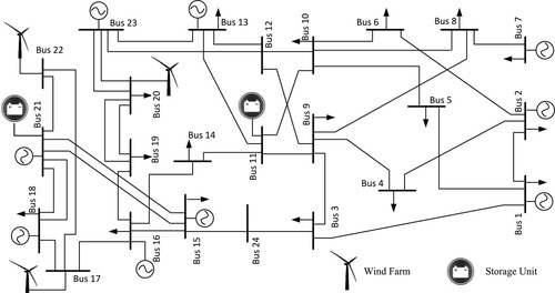
In this section, we consider the modified IEEE 24-bus test system [25], as shown in Figure 11.4. At any hour, the maximum total load in the system is 2850 MW. There are three wind farms with 150, 70, and 30 wind turbines at buses 22, 17, and 11, respectively. Each wind turbine is assumed to have a maximum generation capacity of 1.5 MW. Therefore, the wind penetration is about 13%. The wind speed across these three wind sites is assumed to be the same, due to relative proximity. The wind-speed data was obtained from the Alternative Energy Institute Wind Test Center [26] for the duration of September to November 2012. The wind-speed probability-distribution curves, such as the one shown in Figure 11.5, was derived separately for every hour of the day. Given the wind-speed probability-distribution curves, we generate 200 daily wind-power generation scenarios for the purpose of our analysis. In order to make our simulations more realistic, 180 scenarios are used as training scenarios to run the standard SUC to obtain the price values used for the storage stochastic bidding optimization, which can be thought of as historical data. The remaining 20 scenarios are used as unseen test scenarios to evaluate the actual operation of the storage unit, after it bids in the DA market during its run time.

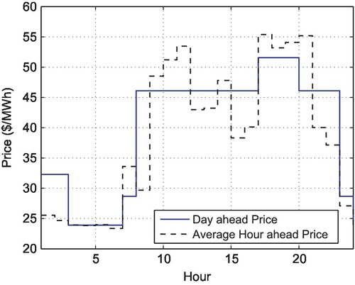
Two independent investor-owned 4.5 MWhs storage units are assumed at buses 21 and 11. The initial charge level for both units is 1.5 MW. The price values for the DA and the HA markets are obtained from the standard SUC analysis that we explained in Section 2. The price curves for the DA energy market, and the average prices in the HA energy markets across all scenarios, at bus 21, are shown in Figure 11.6. Depending on the scenarios, the HA prices may go up to $215/MWh. The price curves for the DA market and for different scenarios of the HA market are used to set the storage bid for purchasing or selling of energy and reserve services in the DA market.
4.2 Stochastic versus Deterministic Design
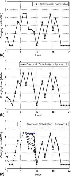
To understand the differences across different design methods, we start by showing the SOC for each method in Figure 11.6. The deterministic optimization method is intended to serve as a base for comparison, where we use the expected values of the HA market prices instead considering each random scenario separately. The two stochastic optimization approaches are those that we proposed in Sections 3.1 and 3.2, respectively. Note that, while the SOC does not change across different scenarios when Approach 1 is used, it does change when Approach 2 is used as shown by different dashed lines for different scenarios in Figure 11.7(c).
4.3 Optimality
Recall from Section 3.2 that our second approach may sometimes be sub-optimal due to the slight differences between the constraints in optimization problems (9) and (26). Therefore, in this section, we examine the optimality of the second approach. The results for 10 different unseen test scenarios are shown in Table 11.1. Here, the optimality loss was calculated based on the difference in the amount of revenue if the unused reserve power is sold only during the peak hours in the hour-ahead market. We can see that for two scenarios, 4 and 9, the exact optimal solution was achieved as there was no need to sell power in any off-peak hour. For the rest of the scenarios, although the solution was sub-optimal, the optimality loss was very minor. on average, the optimality loss across all 10 scenarios is only 3.367%.
Table 11.1
Actual Hour-Ahead Operation of the Storage Unit for 10 Unseen Test Scenarios
| Scenario Number | 1 | 2 | 3 | 4 | 5 | 6 | 7 | 8 | 9 | 10 |
| Power Sold at Peak Hours (MW) | 7.08 | 6.52 | 7.13 | 4.09 | 7.08 | 7.06 | 6.72 | 6.92 | 4.23 | 7.12 |
| Power Sold at Off-Peak Hours (MW) | 0.93 | 0.46 | 0.88 | 0 | 0.89 | 0.95 | 0.70 | 0.63 | 0 | 0.61 |
| Optimality Loss (%) | 4.37 | 3.53 | 4.69 | 0 | 4.54 | 4.45 | 4.78 | 3.73 | 0 | 3.67 |

4.4 Day-ahead versus Hour-ahead Operation
In this section, we take a closer look at the operation of the storage unit in the DA and the HA markets based on an example solution that we obtained by using our second approach. The DA energy and reserve bids in this example are shown in Figure 11.8(a). Here, any negative bar indicates charging of the batteries in an hour h, where Ph < 0 and Rh = 0. In contrast, any positive bar indicates discharging of the batteries in an hour h, where Ph ≥ 0 and Rh ≥ 0. Recall that the exact utilization of the reserve power and the amount of power sold in the HA market are determined later during the operation time. Therefore, different operation scenarios can lead to different outcomes when it comes to the participation of the storage unit in the HA market. Three examples based on three different scenarios are shown in Figures 11.8(b) and (c). We can see that, at each hour, the amount of reserve that is sold in the HA market is always upper bounded by the amount of reserve that the storage unit is committed to in the DA market, i.e., rr,h ≤ Rh for any scenario k. Moreover, the unused reserve power that is sold in the HA market, i.e., ph,k, is almost always sold during the peak hours to maximize the storage unit’s profit.

4.5 Impact of Increasing the Storage Capacity
The daily revenue obtained using various design approaches are shown in Figure 11.9, where the storage capacity grows from 4.5 MW to 4.5 × 10 = 45 MW. We can see that both stochastic optimization approaches outperform deterministic optimization, while the second stochastic optimization approach outperforms the first stochastic optimization approach. The performance gains maintain across all storage-capacity scenarios. When the storage size is as high as 50 MW, the merit of using our proposed approaches become particularly evident.

4.6 Optimal Storage Capacity Planning
The results in Figure 11.9 can also be used for optimal-capacity planning of investor-owned storage units by examining both revenue and cost. This issue is better illustrated in Figure 11.10, where we have plotted the net daily profit, i.e., the revenue minus the cost, versus the size of the storage units. The battery-investment cost was obtained per cycle of charge and discharge for units with WB-LYP1000AHA lithium-ion 1000 Ah battery modules with 3.2 V discharge voltage [27]. The lifetime of the batteries was assumed to be 12000 cycles and the listed price was $1660 per module, which we assumed to decrease to $1000 as more batteries are installed. We can see that there is a trade-off between revenue and cost and the optimal profit can be reached for certain sizes of the storage system.

4.7 Impact of Location
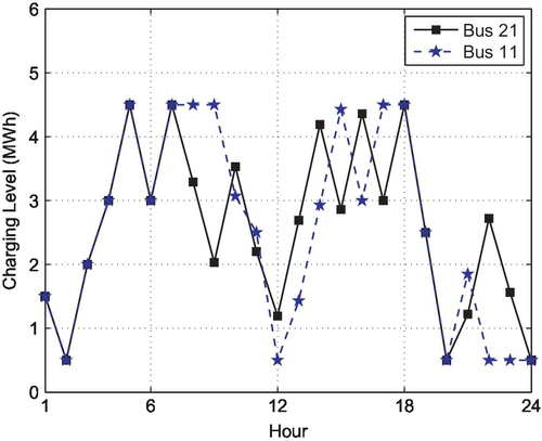
Next, we investigate the impact of location for the storage unit with respect to the revenue achieved. In this regard, we run the simulations for 24 different scenarios, each for a case where the storage unit is assumed to be located at one of the 24 different buses in the system. The results are shown in Figure 11.11. We can see that different buses provide different opportunities for the storage units, making it more desirable to build the storage unit at certain locations. The differences are mainly due to changes in the LMPs at different buses, which is caused by different line-congestion scenarios. In our study, in order to see the effect of line congestions, the capacity of some of the 500 MW transmission lines of the standard test system was reduced to 200 MW. Note that the results in Figure 11.11 are based on the first stochastic optimization approach, i.e., by solving optimization problem (16). That is, we separately obtained the optimal bids and charge/discharge schedules for the case of placing the storage unit at each of the buses. As an example, the charging level when the storage unit is located at buses 21 and 11 are separately plotted in Figure 11.12.

5 Conclusions
Integration of large-scale storage systems in the power system is a key component of future smart grids. In this chapter, a novel approach was proposed to optimally operate such storage systems that are owned by independent private investors. In particular, we proposed an optimal-bidding mechanism for storage units to offer both energy and reserve in the day- ahead and the HA markets when significant fluctuation exists in the market prices due to high penetration of wind and intermittent renewable energy resources. Our design was based on formulating a stochastic programming framework to select different bidding variables. We showed that the formulated optimization problem can be transformed into convex-optimization problems that are tractable and appropriate for implementation. We showed that accounting for the unpredictable feature of market prices due to wind-power fluctuations can improve the decisions made by large storage units, hence increasing their profit. We also investigated the impact of various design parameters, such as the size and location of the storage unit on increasing the profit.
Appendix
First, we explain the new set of notations that we need in order to formulate and solve the standard stochastic unit-commitment problem. C(.) denotes the cost of a particular service. Comii,h denotes commitment of the ith unit in hour h. Pi,h denotes generation of the ith unit in hour h. Ri,h denotes reserve commitment of the ith unit in hour h. Pi+ denotes the maximum capacity of the ith unit. Pi– denotes the minimum capacity of the ith unit. Rampi+ denotes the maximum ramp-up of the ith unit. Rampi– denotes the maximum ramp down of the ith unit. Gf denotes the subset of the fast generators. pi,k,h denotes the generation of the ith fast unit in the hour-ahead market for hour h and scenario k. ri,k,h denotes the reserve usage of the ith unit in the hour-ahead market for hour h and scenario k. NLk,h denotes the total net load in hour h of scenario k, which is the actual demand minus the wind-power generation. Given these notations and parameters, we can now formulate the standard SUC as follows, in which the realization scenarios are considered in order to minimize the expected value of the unit commitment cost in the system:

The above SUC is a mixed-integer program. In general, mixed-integer programs are difficult to solve, although some classes of mixed-integer programs can be solved, e.g., using commercial optimization packages such as MOSEK and CPLEX software [2]. Alternatively, we can relax the binary constraint, solve problem (27), which is a convex-optimization problem after the binary constraints are relaxed, and then set Comi,h = 1 for any i and h with the highest Comi,h. If we repeat this operation until any Comi,h in the solution is either zero or one, we can obtain a feasible but sub-optimal solution for the original problem (27). We used the latter approach. Given the solution and the Lagrange multipliers corresponding to each constraint, the needed system parameters are calculated accordingly, as we have already explained at the end of Section 2. Note that the above problem is solved in centralized fashion. We also note that since the storage units are assumed to have no impact on prices, this optimization problem does not include any variable from the storage units.