Search in book...
Toggle Font Controls
Create new playlist

Name your new playlist

Playlist description (optional)
Sign In

Email address

Password

Forgot Password?

or

Continue with Facebook

Continue with Google
Sign Up

Full Name

Email address

Confirm Email Address

Password

or

Continue with Facebook

Continue with Google

Chapter 6

Incorporating Short-Term Stored Energy Resource into MISO Energy and Ancillary Service Market and Development of Performance-Based Regulation Payment

Yonghong Chen; Marc Keyser; Matthew H. Tackett; Ryan Leonard; Joe Gardner Midcontinent Independent System Operator, Inc. (MISO) Carmel, IN, USA 46032

Abstract

This chapter analyzes various approaches to incorporate short-term stored energy resources (SERs) into MISO co-optimized energy and ancillary service market. Based on analysis, the best approach is to utilize short-term storage energy resources for regulating reserve with the real-time energy dispatch of the SERs to be set in such a way that the maximum regulating reserve on SERs can be cleared. It also introduces the implementation of market based regulation performance payment. The purpose of the enhancement is to provide fair compensation for resources such as SERs that can provide fast and accurate responses.

Keywords

Market design

Ancillary services

Co-optimization

Dispatch and scheduling

Locational marginal price

Market Clearing Price

Reserve

Stored energy resource

1 Introduction

As the regional transmission organization (RTO) and balancing authority (BA), MISO is responsible for reliable and economical procurement of energy, regulating reserve, and contingency reserves as well as utilizing automatic generation control (AGC) to meet North American Electric Reliability Corporation (NERC) standards for BAs.

In February 2007, the Federal Energy Regulatory Commission (FERC) issued order No. 890 [1] to ensure participation of non-generation resources in Independent System Operator (ISO) markets on a fair and equitable basis. When MISO started its energy market in April 2005, the energy market tariff allowed demand response resources (DRR) to bid into the energy market. With the start of the energy and ancillary service market in January 2009, the tariff further separated DRR into two types to allow better participation in the energy and/or ancillary service markets. MISO also included in its energy and ancillary services tariff the means for implementation of energy-storage technologies into the market. The provision to allow short-term stored-energy resources (SER) to participate in the regulating reserve market was implemented in January 2010.

There are various types of energy storages, such as pumped storage generators, compressed air storage, batteries, and flywheels [2]. One of the important characteristics of storage devices is the discharge time at rated power (DTRP) [3]. Devices with DTRP in the range of hours can be handled similar to pumped-storage resources. Such resources can provide energy, contingency reserves, and regulating reserves. Adequate unit commitment and economic dispatch algorithms are required to effectively utilize the limited storage in both the operation planning and dispatch stages. Devices with DTRP less than 5 minutes will be difficult to manage by MISO’s market system with a real-time dispatch interval of 5 minutes. The focus of the chapter is on the so-called short-term SER. This specific type of stored-energy resources typically has a DTRP less than an hour but greater than the real-time dispatch interval, so that it can be effectively considered by real-time security-constrained economic dispatch (SCED) software.

The short-term SER has several unique characteristics that can benefit the energy and ancillary service markets. First of all, SERs are usually very fast to respond and can provide significant value for regulation response in AGC. Pacific Northwest National Laboratory (PNNL) compared the performance of fast-responsive storage resources with conventional regulation resources like hydro, combustion turbines, steam turbines, and combined-cycle units in the California ISO market [4]. The conclusion is that the faster response resources can help reduce California ISO’s regulation procurement by up to 40% on average. The second important benefit of short-term SER is that it can help reduce CO₂ emissions. In [5], KEMA reported on a study of Beacon Power’s flywheel technology in PJM, California ISO, and ISO New England. The conclusion is that flywheel-based frequency regulation can be expected to produce significantly less CO₂ emissions for all three regions.

Because of these benefits, many RTOs have been working on integrating short-term storage resources into their market systems. New York ISO (NYISO) created a resource type called “limited energy stored resources (LESR)” [6]. ISO New England and California ISO have developed pilot programs for this new technology to participate in their regulating reserve markets.

In October 2011, the FERC further issued order No. 755 requiring a two-part payment for regulation resources to account, in part, for accuracy in responding to a transmission system operator’s AGC signal. The two parts of the payment to compensate regulation resources include a market-based capacity payment and a market-based payment for performance (or mileage). The uniform market-based capacity payment also includes a marginal unit’s opportunity costs for keeping a resource’s capacity in reserve in the event that it is needed to provide real-time frequency regulation service. The market-based performance (mileage) payment should reflect the amount of work each resource performs in real-time in response to the system operator’s dispatch signal [7].

Under MISO’s energy and ancillary service market that started in 2009, energy is co-optimized with operating reserves [8]. Operating reserve includes regulating reserve and contingency reserve. Contingency reserve further includes spinning reserve and supplemental reserve. Market participants submit energy offers (including startup cost, no load cost, and incremental energy offer), regulating reserve offers and contingency reserve offers. All reserve offers are in $/MW/h. Under MISO’s market rules, regulating reserve is cleared for deployment in both up and down directions. The regulating reserve market-clearing price (MCP) resulting from the co-optimization include the marginal units’ opportunity costs and is used to pay for the cleared regulating capacity. However, prior to FERC order 755, there was no compensation for the movement of regulation. With the same cleared regulation capacity, fast-ramping resources can respond to AGC regulation deployment signals quicker than slower-ramping resources, and tend to provide more movement for regulation. Hence, order No. 755 requires a fair compensation for “the inherently greater amount of frequency regulation service being provided by faster-ramping resources.”

MISO complied with order No. 755 by enhancing its market rules with a two-part payment calculation to compensate resources that provide regulating reserve. This enhancement was implemented in December 2012.

This chapter presents the studies and analysis that led to the market design for incorporating short-term SERs into the MISO market [9] and the development of performance-based regulation payment [10].

2 Market-Product Qualification and Market-Clearing Price on Short-term SER

2.1 Market-Product Qualification

The MISO energy and ancillary service market clears energy and operating reserves. In MISO’s market, the operating reserve consists of regulating reserve and contingency reserve. Regulating reserve is cleared for AGC deployment on a 4-second basis. Contingency reserve consists of spinning reserve and supplemental reserve. These products are cleared in order to be able to respond in the event of a system contingency. Overall, the ancillary service market procures three types of reserve products – regulating reserve, spinning reserve, and supplemental reserve. The qualification and deployment requirements of the three types of reserve products are defined in the tariff [8].

A short-term SER can only provide a very limited amount of sustained energy before it needs to be charged. Hence, it is not suited for an energy product. Based on the NERC’s 90 minutes contingency reserve restoration period requirement following a contingency event [11], a short-term SER is not suited for contingency reserves either. Therefore, in MISO’s tariff, the short-term SER is only allowed to provide regulating reserves. In MISO’s market design, regulating reserve is a higher-quality product than contingency reserves and it can substitute for contingency reserves. To prevent regulating reserves cleared from short-term SERs to substitute for contingency reserves, a constraint is added to ensure that the total amount of regulation cleared on short-term SERs is no more than the market-wide regulating reserve requirement. This constraint has implications on the regulating reserve MCP for short-term SERs.

MISO also enforces zonal reserve constraints. Within each zone, regulating reserve can substitute for contingency reserve. Zonal contingency reserve requirements come from deliverability studies. The purpose is to ensure enough contingency reserves inside each zone so that the amount of contingency deployment imported from outside the zone will not cause transmission congestion. If short-term SERs are allowed to meet zonal regulating reserve requirements, they can potentially be used to substitute for zonal contingency reserves. After a short time period, likely less than the disturbance recovery period, the storage will deplete, and the zone will need additional import from outside to replace the deployment from short-term SERs. For this reason, short-term SERs are not allowed to meet zonal regulating reserve requirements.

2.2 Optimization constraints and MCP

Under MISO’s day-ahead (DA) commitment and dispatch, its reliability assessment commitment (RAC) [12], and its look-ahead commitment (LAC) [13], energy is co-optimized with regulating and contingency reserves in the security-constrained unit commitment (SCUC) and the DA-SCED software. Under MISO’s real-time dispatch [14], energy is also co-optimized with regulating and contingency reserves every 5 minutes in the RT-SCED software.

A simplified MISO RT-SCED formulation is used here to explain how energy and reserve products are co-optimized in the market-clearing processes. This simplified model does not include constraints such as special handling of demand response resources, penalty terms or reserve demand curves, etc. These simplifications reduce the complexity that is not directly related to the problem under discussion.

Without short-term SERs, the RT-SCED optimization problem for the solution interval t can be described as follows:

${Min}_{p, r} \sum_{jϵJ} \{C_{j, t}^{P} (p_{j}^{t}) + \sum_{x \in X} ({O_{j, t}^{x} \cdot r}_{j}^{x, t})\}$ ${Min}_{p, r} \sum_{jϵJ} \{C_{j, t}^{P} (p_{j}^{t}) + \sum_{x \in X} ({O_{j, t}^{x} \cdot r}_{j}^{x, t})\}$

Subject to:

Market-wide or zonal constraints (shadow price):

Power-Balance Equation with losses (λ_t)

$\sum_{jϵJ} \{p_{j, t} \cdot (1 - Λ_{n_{j}, t})\} + \sum_{nϵN} \{P_{n, t} \cdot (1 - Λ_{n, t})\} - ▵_{t}^{LOSS} = 0$ $\sum_{jϵJ} \{p_{j, t} \cdot (1 - Λ_{n_{j}, t})\} + \sum_{nϵN} \{P_{n, t} \cdot (1 - Λ_{n, t})\} - ▵_{t}^{LOSS} = 0$

(1)

In RT SCED, losses are linearized around the SE snapshot. Δ_t^LOSS reflects the difference between state estimation (SE) AC losses and the corresponding marginal losses calculated by using loss sensitivities and SE injections and withdrawals [15].

Transmission Constraints (μ_i,t)

$\sum_{j \in J} \{p_{j, t} \cdot B_{i, n_{j}, t}\} + \sum_{n \in N} \{P_{n, t} \cdot B_{i, n, t}\} + ▵_{i, t}^{FLOW} \leq {\bar{F}}_{i, t} \forall i \in I$ $\sum_{j \in J} \{p_{j, t} \cdot B_{i, n_{j}, t}\} + \sum_{n \in N} \{P_{n, t} \cdot B_{i, n, t}\} + ▵_{i, t}^{FLOW} \leq {\bar{F}}_{i, t} \forall i \in I$

(2)

In RT SCED, transmission flows are linearized around the SE snapshot. Δ_i,t^FLOW reflects the difference between SE AC flow and the corresponding flow calculated by using flow-sensitivity factors and SE injections and withdrawals [15].

Market-wide regulating reserve requirement (γ_t^MRR)

$\sum_{j \in J} (r_{j, t}^{REG}) \geq R_{MKT, t}^{REG}$ $\sum_{j \in J} (r_{j, t}^{REG}) \geq R_{MKT, t}^{REG}$

(3)

Market-wide regulating plus spinning reserve requirement (γ_t^MRS)

$\sum_{j \in J} (r_{j, t}^{REG} + r_{j, t}^{SPIN}) \geq R_{MKT, t}^{REG} + R_{MKT, t}^{SPIN}$ $\sum_{j \in J} (r_{j, t}^{REG} + r_{j, t}^{SPIN}) \geq R_{MKT, t}^{REG} + R_{MKT, t}^{SPIN}$

(4)

Market-wide operating reserve requirement (γ_t^MOR)

$\sum_{j \in J} (\sum_{x \in X} r_{j, t}^{x}) \geq \sum_{x \in X} R_{MKT, t}^{x}$ $\sum_{j \in J} (\sum_{x \in X} r_{j, t}^{x}) \geq \sum_{x \in X} R_{MKT, t}^{x}$

(5)

Zonal regulating reserve requirement (γ_k,t^ZRR)

$\sum_{j \in J^{k}} (r_{j, t}^{REG}) \geq R_{k, t}^{REG} \forall k \in K$ $\sum_{j \in J^{k}} (r_{j, t}^{REG}) \geq R_{k, t}^{REG} \forall k \in K$

(6)

Zonal regulating plus spinning reserve requirement (γ_k,t^ZRS)

$\sum_{j \in J^{k}} (r_{j, t}^{REG} + r_{j, t}^{SPIN}) \geq R_{k, t}^{REG} + R_{k, t}^{SPIN} \forall k \in K$ $\sum_{j \in J^{k}} (r_{j, t}^{REG} + r_{j, t}^{SPIN}) \geq R_{k, t}^{REG} + R_{k, t}^{SPIN} \forall k \in K$

(7)

Zonal operating reserve requirement (γ_k,t^ZOR)

$\sum_{j \in J^{k}} (\sum_{x \in X} r_{j, t}^{x}) \geq \sum_{x \in X} R_{k, t}^{x} \forall k \in K$ $\sum_{j \in J^{k}} (\sum_{x \in X} r_{j, t}^{x}) \geq \sum_{x \in X} R_{k, t}^{x} \forall k \in K$

(8)

Resource-level constraints:

Limit constraints and ramp constraints:

$p_{j, t} + \sum_{x \in X} r_{j, t}^{x} \leq U_{j, t} \cdot {\bar{P}}_{j, t} \forall j \in J$ $p_{j, t} + \sum_{x \in X} r_{j, t}^{x} \leq U_{j, t} \cdot {\bar{P}}_{j, t} \forall j \in J$

$p_{j, t} {- r}_{j, t}^{REG} \geq U_{j, t} \cdot {\underline{P}}_{j, t} \forall j \in J$ $p_{j, t} {- r}_{j, t}^{REG} \geq U_{j, t} \cdot {\underline{P}}_{j, t} \forall j \in J$

$- L_{t} \cdot V_{j, t}^{DOWN} \leq p_{j, t} - P_{j, t 0} \leq L_{t} \cdot V_{j, t}^{UP} \forall j \in J$ $- L_{t} \cdot V_{j, t}^{DOWN} \leq p_{j, t} - P_{j, t 0} \leq L_{t} \cdot V_{j, t}^{UP} \forall j \in J$

${0 \leq r}_{j, t}^{x} \leq {\bar{R}}_{j, t}^{x} \forall x \in X, \forall j \in J$ ${0 \leq r}_{j, t}^{x} \leq {\bar{R}}_{j, t}^{x} \forall x \in X, \forall j \in J$

Under this formulation, market-wide and zonal reserve MCPs are calculated as:

${MCP}_{MKT, t}^{REG} = γ_{t}^{MRR} + γ_{t}^{MRS} + γ_{t}^{MOR}$ ${MCP}_{MKT, t}^{REG} = γ_{t}^{MRR} + γ_{t}^{MRS} + γ_{t}^{MOR}$

(9)

${MCP}_{MKT, t}^{SPIN} = γ_{t}^{MRS} + γ_{t}^{MOR}$ ${MCP}_{MKT, t}^{SPIN} = γ_{t}^{MRS} + γ_{t}^{MOR}$

(10)

${MCP}_{MKT, t}^{SUPP} = γ_{t}^{MOR}$ ${MCP}_{MKT, t}^{SUPP} = γ_{t}^{MOR}$

(11)

${MCP}_{k, t}^{REG} = γ_{t}^{MRR} + γ_{t}^{MRS} + γ_{t}^{MOR} + γ_{k, t}^{ZRR} + γ_{k, t}^{ZRS} + γ_{k, t}^{ZOR}$ ${MCP}_{k, t}^{REG} = γ_{t}^{MRR} + γ_{t}^{MRS} + γ_{t}^{MOR} + γ_{k, t}^{ZRR} + γ_{k, t}^{ZRS} + γ_{k, t}^{ZOR}$

(12)

${MCP}_{k, t}^{SPIN} + γ_{t}^{MRS} + γ_{t}^{MOR} + γ_{k, t}^{ZRS} + γ_{k, t}^{ZOR}$ ${MCP}_{k, t}^{SPIN} + γ_{t}^{MRS} + γ_{t}^{MOR} + γ_{k, t}^{ZRS} + γ_{k, t}^{ZOR}$

(13)

${MCP}_{k, t}^{SUPP} = γ_{t}^{MOR} + γ_{k, t}^{ZOR}$ ${MCP}_{k, t}^{SUPP} = γ_{t}^{MOR} + γ_{k, t}^{ZOR}$

(14)

${LMP}_{n, t} = λ_{t} (1 - Λ_{n, t}) + \sum_{i \in I} \{μ_{i, t} \cdot B_{i, n, t}\}$ ${LMP}_{n, t} = λ_{t} (1 - Λ_{n, t}) + \sum_{i \in I} \{μ_{i, t} \cdot B_{i, n, t}\}$

(15)

$\forall k \in K, \forall n \in N$ $\forall k \in K, \forall n \in N$

where:

j – Index of all resources

n – Index of all nodes in the network

t – Index of dispatch interval

i – Index of transmission constraints

x – Index of all reserve categories including regulating reserve (REG), spinning reserve (SPIN), and supplemental reserve (SUPP)

J – Set of resources

N – Set of nodes in the network

K – Set of reserve zones

I – Set of transmission constraints

X – Set of reserve categories {REG, SPIN, SUPP}

J^k– Set of resources in zone k ∈ K

R_MKT,t^x – Market-wide requirement for reserve x at t

R_k,t^x – Zone k requirement for reserve x at t

B_i,n,t – Sensitivity of the flow on transmission constraint i to injection at node n and withdrawal at the reference bus

Λ_n,t – Sensitivity of system losses to injection at node n and withdrawal at the reference bus

P_n,t – Net fixed injection at node n

P_t – Vector of net fixed injection

Δ_t^LOSS – System loss linearization offset

Δ_i,t^FLOW – Transmission constraint i flow linearization offset

n_j – The node at which resource j is located

${\bar{F}}_{i, t}$ ${\bar{F}}_{i, t}$ – Limit for transmission constraint i

O_j,t^x – Resource j available offer price for reserve x, in $/MW/h

${\bar{P}}_{j, t}$ ${\bar{P}}_{j, t}$ – Resource j maximum power output at interval t

${\underline{P}}_{j, t}$ ${\underline{P}}_{j, t}$ – Resource j minimum power output at interval t

${\bar{R}}_{j, t}^{x}$ ${\bar{R}}_{j, t}^{x}$ – Maximum amount of reserve x that can be cleared on resource j, 0 if resource j is not qualified for providing reserve x

L_t – Interval length of interval t, in minutes

V_j,t^UP – Resource j up ramp rate in MW/Min

V_j,t^DOWN – Resource j down ramp rate in MW/Min

P_j,t0 – Resource j energy dispatch target from previous interval; for single-interval SCED, this is a given parameter.

U_j,t – Binary parameter that is 1 when resource j is committed and online dispatchable for interval t, 0 otherwise

p_j,t – Cleared energy on resource j

p_t – Vector of cleared energy

r_j,t^x – Cleared reserve x on resource j

C_j,t^P(·) – Energy offer cost function from resource j, in $/h. It is a function of p_j,t_.

MCP_MKT,t^x – Market-wide MCP for reserve x

MCP_k,t^x – Zonal MCP for reserve x in zone k

LMP_n,t – LMP at node n

In this formulation, a higher-quality reserve product can substitute for a lower-quality reserve product. Regulating reserves can substitute for spinning reserves and spinning reserves can substitute for supplemental reserves. Resources in each zone are paid at the zonal reserve MCPs for cleared reserves. It has the property that: ${MCP}_{k, t}^{REG} \geq {MCP}_{k, t}^{SPIN} \geq {MCP}_{k, t}^{SUPP} \geq 0, \forall k \in K .$ ${MCP}_{k, t}^{REG} \geq {MCP}_{k, t}^{SPIN} \geq {MCP}_{k, t}^{SUPP} \geq 0, \forall k \in K .$

By introducing the short-term SER, cleared regulating reserve on short-term SERs can meet requirements in constraints (3), (4), and (5). To prevent short-term SERs from substituting for spinning or supplemental reserves, a new constraint called “market-wide short-term SER regulating reserve constraint” is introduced to ensure that total cleared regulation on short-term SERs is no more than the market-wide regulating reserve requirement:

$\sum_{s \in S} (r_{s, t}^{REG}) \leq R_{MKT, t}^{REG}$ $\sum_{s \in S} (r_{s, t}^{REG}) \leq R_{MKT, t}^{REG}$

(16)

where:

s Index of SERs

S Set of SERs

In (16), r_s,t^REG is the regulating reserve cleared on short-term SER s at interval t. Denote the shadow price for this constraint as γ_t^MSERR. It is negative when the constraint is binding. The MCP for regulating reserve cleared on short-term SER is:

${MCP}_{SER, t}^{REG} = γ_{t}^{MRR} + γ_{t}^{MRS} + γ_{t}^{MOR} + γ_{t}^{MSERR}$ ${MCP}_{SER, t}^{REG} = γ_{t}^{MRR} + γ_{t}^{MRS} + γ_{t}^{MOR} + γ_{t}^{MSERR}$

(17)

When zonal reserve constraints (6) ~ (8) and the market-wide short-term SER regulating reserve constraint (17) are not binding, short-term SERs and all the other generation-based resources have the same regulating reserve MCP. The regulating reserve MCP is no less than the spinning reserve MCP and the spinning reserve MCP is no less than the supplemental reserve MCP. Under market-wide regulating reserve scarcity, regulating reserve scarcity price will be reflected into MCP_SER,t^REG. Under market-wide regulating plus spinning reserve scarcity or market-wide operating reserve scarcity, the corresponding scarcity prices will also be reflected into MCP_SER,t^REG as long as not all the market-wide regulating reserve requirement is served by short-term SERs, i.e., constraint (16) is not binding. The reason is that clearing more regulating reserve on short-term SERs can free up regulating reserve on other resources so that they can be used to substitute spinning reserve or supplemental reserves.

When zonal reserve constraints (6) ~ (8) are binding, the regulating reserve MCP for the binding zones will be higher than MCP_SER,t^REG. The reason is that short-term SERs cannot meet the zonal reserve requirement and more expensive reserves on other types of resources need to be cleared to meet zonal requirements.

When zonal reserve constraints (6) ~ (8) are not binding but the “market-wide short-term SER regulating reserve constraint” (16) is binding, i.e., all market-wide regulating reserve requirement is met by short-term SERs, MCP_SER,t^REG can be less than the spinning or supplemental reserve MCP. The reason is that the lower cost regulation from short-term SERs cannot substitute for spinning or supplemental reserves. In this scenario, even if there is market-wide regulating plus spinning reserve or market-wide operating reserve scarcity, the scarcity prices will not be reflected into MCP_SER,t^REG because regulating reserve from short-term SERs can neither substitute for spinning or supplemental reserves nor help to free up regulating reserve on other resources to substitute for spinning or supplemental reserves.

2.3 Example 1: SER regulating reserve MCP

Figure 6.1 shows a 5-bus system with SER.

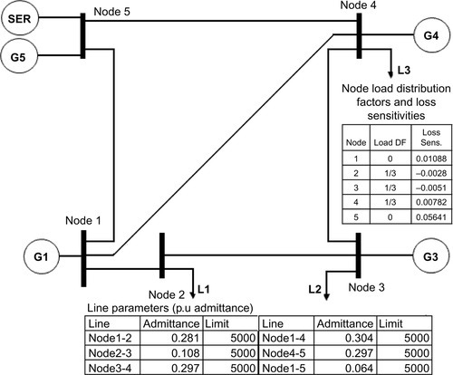
f06-01-9780124104914 — Figure 6.1 5-Bus System.

• G1 ~ G5 are all in zone 1, and there is only one zone.

• Assume all resources are online and qualified for regulating and spinning reserve. The market-wide contingency reserve requirement can be met by spinning reserves and there is no requirement for supplemental reserves.

• In the RT-SCED algorithm, fix the SER energy dispatch at 0 MW and allow the regulation to be cleared within its limit ranging from −75MW to 75MW based on the regulation offer price of $1/MW/h.

The input data for RT-SCED is shown in Table 6.1. Table 6.2 shows the solution from RT-SCED. In this special scenario, the regulation offer is cheaper than contingency reserve offers. Therefore, more than the required 71 MW of regulation is cleared to substitute for contingency reserve. Even though the regulation from the SER is the cheapest at $1/MW/h, it is only cleared up to the market-wide regulating reserve requirement, 71 MW. The shadow price γ_t^MOR = 7 and γ_t^MSERR = −6. The MCP for the SER is MCP_SER,t^REG = 1 and it is the price paid for the 71 MW regulation cleared on SER. The MCPs for other resources are:

${MCP}_{“ 1, ” t}^{REG} = {MCP}_{“ 1, ” t}^{SPIN} = {MCP}_{“ 1, ” t}^{SUPP} = 7 .$ ${MCP}_{“ 1, ” t}^{REG} = {MCP}_{“ 1, ” t}^{SPIN} = {MCP}_{“ 1, ” t}^{SUPP} = 7 .$

Table 6.1

Input Data for Example 1

Unit	Node	Offer			Power Output Limit (MW)		Ramp Rate MW/Min	Zone	Energy Target from previous Interval
Unit	Node	Energy ($/MW/h)	Regulating Reserve ($/MW/h)	Contingency Reserve ($/MW/h)	Min	Max	Ramp Rate MW/Min	Zone	Energy Target from previous Interval
G1	1	14	1.9	4.62	0	110	10	1	110
G3	3	30	4.5	7	0	520	20	1	67
G4	4	31	4.65	10.23	0	200	10	1	70
G5	5	10	1.5	5.3	0	600	30	1	450
SER	5	N/A	1	N/A	−75	75	1000	N/A	0

t0010

Table 6.2

Example 1 Clearing Results

Load	670 MW	Market wide Regulating Reserve Requirement	Market wide Contingency Reserve Requirement
Solved Losses	34.92 MW	71 MW	81 MW
Unit	Cleared Energy (MW)	Cleared Regulating reserve(MW)	Cleared Contingency reserve(MW)
G1	84.92	25.08	0
G3	0	0	36.92
G4	20	20	0
G5	600	0	0
SER	0	71	0
Total	704.92	116.08	36.92

t0015

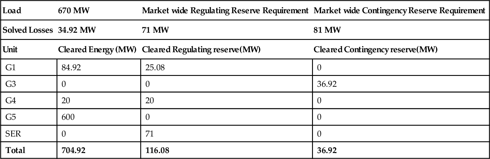
The regulation cleared on G1 and G4 are used to substitute for contingency reserves. Therefore, the regulating reserve MCP on generation resources is the same as the spinning and supplemental reserve MCPs.

3 Real-Time Dispatch

In MISO’s real-time market, energy is co-optimized with regulating reserve and contingency reserve in RT-SCED every 5 minutes. Even though short-term SERs only provide regulating reserve, the energy dispatch is critical to the procurement of regulating reserve. This section introduces the physical parameters of short-term SERs and how their capacity limits are dynamically calculated for RT-SCED. Three options that have been studied on the energy dispatch are analyzed, and option 3 is chosen.

3.1 Physical parameters and capacity limit calculation

A short-term SER needs to provide the following physical parameters for a dispatch interval:

(a) ${\bar{P}}_{s, t}^{PHY}$ ${\bar{P}}_{s, t}^{PHY}$ , ${\underline{P}}_{s, t}^{PHY}$ ${\underline{P}}_{s, t}^{PHY}$ – Maximum and minimum physical power output, i.e., the MW of power that a SER can physically output without storage limitation. Minimum power output can be negative

(b) ${\bar{P}}_{s, t}$ ${\bar{P}}_{s, t}$ , ${\underline{P}}_{s, t}$ ${\underline{P}}_{s, t}$ – Maximum and minimum power output at interval t based on actual energy storage level (in MW)

(d) ${\bar{ESL}}_{s, t}$ ${\bar{ESL}}_{s, t}$ – Maximum energy storage level (in MWh)

(e) ER_s,t^CHG– Maximum energy that the resource can be charged during a 1-minute time period (in MWh/Min)

(f) ER_s,t^DCHG– Maximum energy that the resource can be discharged during a one-minute time period (in MWh/Min)

(g) ER_s,t^LOSS– Energy lost during a 1-minute time period, inherent to the system (in MWh/Min)

(h) ER_s,t^FWDR– Maximum full charge energy withdrawal rate. Used to model additional capability for withdrawal of energy by adding, for example, resistors (in MWh/Min).

In addition, the RT-SCED algorithm needs to know the energy storage level ESL_s,t0^ICCP and the MW output P_s,t0^ICCPat time t₀ when the case starts to execute. These two are instantaneous real-time measurements sent to the RTO via inter-control center communications protocol (ICCP). P_s,t0^ICCP is used by the state estimator to solve for the state-estimation output P_s,t0^SE.

The RT-SCED case that starts at t₀ solves for target time t = t₀ + 10. The case solves every 5 minutes. Between [t_0, t₀ + 5], the resource is expected to follow the dispatch from the previous RT-SCED solution. Assume the cleared energy and regulating reserve from the previous interval solution are P_j,t0 + 5 and r_j,t0 + 5^REG, respectively.

To solve for the p_j,t0 + 10 and r_j,t0 + 10^REG, the maximum and minimum limit for the SER between [t₀+ 5, t₀+ 10] must be determined. These limits change with the storage level. There are three steps to calculate the limits:

1. Calculate the maximum and minimum possible MW output between [t₀, t₀+ 5] based on P_s,t0^SE, P_j,t0 + 5, and r_j,t0 + 5^REG. Assuming the SER follows RTO set points, its output should come from the energy dispatch and regulation deployment from AGC. The maximum and minimum output that the SER can reach at t₀+ 5 are:

${HMW}_{s, t 0 + 5} = {Min (P_{s, t 0 + 5} + SERRegDeployfactor \cdot r}_{s, t 0 + 5}^{REG}, P_{s, t 0}^{SE} + 5 \cdot V_{s, t 0 + 5});$ ${HMW}_{s, t 0 + 5} = {Min (P_{s, t 0 + 5} + SERRegDeployfactor \cdot r}_{s, t 0 + 5}^{REG}, P_{s, t 0}^{SE} + 5 \cdot V_{s, t 0 + 5});$

${LMW}_{s, t 0 + 5} = {Max (P_{s, t 0 + 5} - SERRegDeployfactor \cdot r}_{s, t 0 + 5}^{REG} {, P}_{s, t 0}^{SE} - 5 \cdot V_{s, t 0 + 5}) .$ ${LMW}_{s, t 0 + 5} = {Max (P_{s, t 0 + 5} - SERRegDeployfactor \cdot r}_{s, t 0 + 5}^{REG} {, P}_{s, t 0}^{SE} - 5 \cdot V_{s, t 0 + 5}) .$

SERRegDeployfactor is a tuning parameter between 0 and 1 that estimates the regulation deployment between [t_0, t₀+ 5]. This parameter will be discussed in detail in Section 5.

2. Calculate the maximum and minimum possible energy storage level at t₀+ 5 based on ESL_s,t0^ICCP and assuming that the SER stays at LMW_s,t0 + 5 and HMW_s,t0 + 5, respectively, between [t₀, t₀+ 5].
The maximum possible storage level (energy storage ceiling) at t₀+ 5 is:

${ESL}_{s, t 0 + 5}^{CEILING} = {Min {\bar{ESL}}_{s, t 0 + 10}, Max (0, {ESL}_{s, t 0}^{ICCP} - 5 \cdot {ER}_{s, t 0 + 5}^{LOSS} - 5 \cdot {LMW}_{s, t 0 + 5} / 60)};$ ${ESL}_{s, t 0 + 5}^{CEILING} = {Min {\bar{ESL}}_{s, t 0 + 10}, Max (0, {ESL}_{s, t 0}^{ICCP} - 5 \cdot {ER}_{s, t 0 + 5}^{LOSS} - 5 \cdot {LMW}_{s, t 0 + 5} / 60)};$

si37_e

The minimum possible storage level (energy storage floor) at t₀+ 5 is:

${ES L}_{s, t 0 + 5}^{FLOOR} = Max \{0, {ESL}_{s, t 0}^{ICCP} - 5 \cdot {ER}_{s, t 0 + 5}^{LOSS} - 5 \cdot {HMW}_{s, t 0 + 5} / 60)\};$ ${ES L}_{s, t 0 + 5}^{FLOOR} = Max \{0, {ESL}_{s, t 0}^{ICCP} - 5 \cdot {ER}_{s, t 0 + 5}^{LOSS} - 5 \cdot {HMW}_{s, t 0 + 5} / 60)\};$

3. Calculate the maximum and minimum MW that the SER can sustainably output between [t₀+ 5, t₀+ 10] under the energy storage floor and ceiling calculated from step 2. The maximum limit is also capped by physical parameters like maximum energy discharge rate and maximum physical power output. Similarly the minimum limit is capped by maximum energy-charge rate and minimum physical-power output.

${\bar{P}}_{s, t 0 + 10} = Min \{12 \cdot Max (0, {ESL}_{s, t 0 + 5}^{FLOOR} - 5 \cdot {ER}_{s, t 0 + 10}^{LOSS}), 60 \cdot {ER}_{s, t 0 + 10}^{DCHG}, {\bar{P}}_{s, t 0 + 10}^{PHY}\};$ ${\bar{P}}_{s, t 0 + 10} = Min \{12 \cdot Max (0, {ESL}_{s, t 0 + 5}^{FLOOR} - 5 \cdot {ER}_{s, t 0 + 10}^{LOSS}), 60 \cdot {ER}_{s, t 0 + 10}^{DCHG}, {\bar{P}}_{s, t 0 + 10}^{PHY}\};$

si39_e

${\underline{P}}_{s, t 0 + 10} = Max \{- 12 \cdot [{\bar{ESL}}_{s, t 0 + 10} + 5 \cdot {ER}_{s, t 0 + 10}^{FWDR} - ({ESL}_{s, t 0 + 5}^{CE I LING} - 5 \cdot {ER}_{s, t 0 + 10}^{LOSS})], - 60 \cdot {ER}_{s, t 0 + 10}^{CHG}, {\underline{P}}_{s, t 0 + 10}^{PHY}\} .$ ${\underline{P}}_{s, t 0 + 10} = Max \{- 12 \cdot [{\bar{ESL}}_{s, t 0 + 10} + 5 \cdot {ER}_{s, t 0 + 10}^{FWDR} - ({ESL}_{s, t 0 + 5}^{CE I LING} - 5 \cdot {ER}_{s, t 0 + 10}^{LOSS})], - 60 \cdot {ER}_{s, t 0 + 10}^{CHG}, {\underline{P}}_{s, t 0 + 10}^{PHY}\} .$

si40_e

${\bar{P}}_{s, t 0 + 10}$ ${\bar{P}}_{s, t 0 + 10}$ and ${\underline{P}}_{s, t 0 + 10}$ ${\underline{P}}_{s, t 0 + 10}$ are used as the limits for solving the target time t=t₀+ 10 energy dispatch and reserve procurement. Three options have been considered for handling the energy dispatch in RT-SCED.

3.2 Real-time energy dispatch options

For all three options, there are no energy offers, spinning reserve offers, or supplemental reserve offers from the short-term SER. The short-term SER can only offer regulating reserve into the market.

Option 1: Co-optimize short-term SER’s energy dispatch with regulating reserve procurement. In this option, both p_s,t0 + 10 and r_s,t0 + 10^REG are primal variables. Since there is no energy offer, only the regulating reserve cost from SER is added into the objective. It essentially treats the SER energy cost as 0.

Since RT-SCED solves for one target time and does not look over future intervals, this option may not manage the storage well to maximize its benefit over longer periods of time. For example, if dispatching the energy up can help relieve a transmission constraint, the energy will be dispatched to the maximum level until the storage is empty in several intervals. After that, if the LMP is not low enough, the SER will not be charged. This outcome can result in a large percentage of idling time for the short-term SER. Hence, it may not be the best use of the regulation capability of short-term SERs.

Option 2: Always preset short-term SER’s energy dispatch at the position that maximizes the regulating reserves that can be cleared. It is similar to the approach used by NYISO [6]. This approach pre-calculates and fixes the SER energy dispatch halfway between the maximum and minimum limits:

$P_{s, t 0 + 10} = 0.5 \cdot ({\underline{P}}_{s, t 0 + 10} + {\bar{P}}_{s, t 0 + 10})$ $P_{s, t 0 + 10} = 0.5 \cdot ({\underline{P}}_{s, t 0 + 10} + {\bar{P}}_{s, t 0 + 10})$

P_s,t0 + 10 is added into the power-balance equation, but it is not a primal variable. r_s,t0 + 10^REG is a primal variable and it can be cleared to the maximum amount supported by the storage level:

$r_{s, t 0 + 10}^{REG} \leq Min \{5 ⁎ V_{s, t 0 + 10}, 0.5 \cdot ({\bar{P}}_{s, t 0 + 10} - {\underline{P}}_{s, t 0 + 10})\}$ $r_{s, t 0 + 10}^{REG} \leq Min \{5 ⁎ V_{s, t 0 + 10}, 0.5 \cdot ({\bar{P}}_{s, t 0 + 10} - {\underline{P}}_{s, t 0 + 10})\}$

The benefit of this approach is that the short-term SER can always be charged or discharged so that the maximum amount of regulation can be cleared and makes the best use of the regulation capability of short-term SERs. However, since the energy dispatch is pre-fixed, this approach may cause reliability and economic issues. For example, the short-term SER can be charged when the price is extremely high. The high price can be caused by transmission congestion or even system shortages, in which case the SER energy dispatch may jeopardize reliable operation of the system. Under this scenario, manual procedures can be introduced to disable SERs from clearing energy. However, this introduces additional burdens on operators.

Option 3: Preset short-term SER’s energy dispatch at the position such that the maximum amount of regulation can be cleared, and also allow the energy dispatch to be violated if needed. This option is evolved from option 2 and adds protection inside the optimization to the potential harm that the pre-fixed energy dispatch may cause. First, the desired energy dispatch is calculated as:

$P_{s, t 0 + 10}^{DESIRED} = 0.5 \cdot ({\underline{P}}_{s, t 0 + 10} + {\bar{P}}_{s, t 0 + 10})$ $P_{s, t 0 + 10}^{DESIRED} = 0.5 \cdot ({\underline{P}}_{s, t 0 + 10} + {\bar{P}}_{s, t 0 + 10})$

Then introduce a new primal slack variable sl_s,t0 + 10 so that P_s,t0 + 10^DESIRED can be moved to 0 if necessary. In the objective, add the term:

${sl}_{s, t 0 + 10} \cdot SEREnergyPenalty$ ${sl}_{s, t 0 + 10} \cdot SEREnergyPenalty$

SEREnergyPenalty is the penalty for violating the constraint. It is set to the same value as the regulating reserve demand curve price. The outcome is that the short-term SER will not be charged or discharged when the marginal cost of the dispatch is more than the regulating reserve demand curve price.

The following set of “SER energy dispatch constraints” is added:

If P_s,t0 + 10^DESIRED ≥ 0 then

$p_{s, t 0 + 10} = P_{s, t 0 + 10}^{DESIRED} - {sl}_{s, t 0 + 10}$ $p_{s, t 0 + 10} = P_{s, t 0 + 10}^{DESIRED} - {sl}_{s, t 0 + 10}$

Else

$p_{s, t 0 + 10} = P_{s, t 0 + 10}^{DESIRED} + {sl}_{s, t 0 + 10}$ $p_{s, t 0 + 10} = P_{s, t 0 + 10}^{DESIRED} + {sl}_{s, t 0 + 10}$

(18)

Endif

$0 \leq {sl}_{s, t 0 + 10} \leq | P_{s, t 0 + 10}^{DESIRED} |$ $0 \leq {sl}_{s, t 0 + 10} \leq | P_{s, t 0 + 10}^{DESIRED} |$

(19)

p_s,t0 + 10 is added into the power-balance equation. The following ramp and limit constraints are enforced for short-term SERs:

$r_{s, t 0 + 10}^{REG} \leq Min \{5 \cdot V_{s, t 0 + 10}, 0.5 \cdot ({\bar{P}}_{s, t 0 + 10} - {\underline{P}}_{s, t 0 + 10})\}$ $r_{s, t 0 + 10}^{REG} \leq Min \{5 \cdot V_{s, t 0 + 10}, 0.5 \cdot ({\bar{P}}_{s, t 0 + 10} - {\underline{P}}_{s, t 0 + 10})\}$

(20)

$p_{s, t 0 + 10} + r_{s, t 0 + 10}^{REG} \leq {\bar{P}}_{s, t 0 + 10}$ $p_{s, t 0 + 10} + r_{s, t 0 + 10}^{REG} \leq {\bar{P}}_{s, t 0 + 10}$

(21)

$p_{s, t 0 + 10} - r_{s, t 0 + 10}^{REG} \geq {\underline{P}}_{s, t 0 + 10}$ $p_{s, t 0 + 10} - r_{s, t 0 + 10}^{REG} \geq {\underline{P}}_{s, t 0 + 10}$

(22)

If in the RT-SCED solution sl_s,t0 + 10 is greater than 0, then set P_s,t0 + 10^DESIRED = p_s,t0 + 10 * (1 − ɛ) and re-solve (ɛ is a very small number).

3.3 Example 2: Comparison of three energy dispatch options

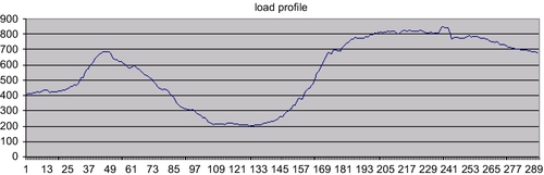
In this example, the 5-bus system in Figure 6.1 is used to sequentially run 291 RT-SCED cases based on the load profile shown in Figure 6.2. The load profile is scaled down based on one day of MISO’s actual load. Assume line “4-5” has a limit of 200MW.

f06-02-9780124104914 — Figure 6.2 Load profile

Assume the following physical parameters for the short-term SER:

${\bar{P}}_{s, t}^{PHY} = 20 MW, {\underline{P}}_{s, t}^{PHY} = - 20 MW, V_{s, t} = 1000 MW / Min, {\bar{ESL}}_{s, t} = 5 MWh, {ER}_{s, t}^{CHG} = {ER}_{s, t}^{DCHG} = 9999 MWh / Min,$ ${\bar{P}}_{s, t}^{PHY} = 20 MW, {\underline{P}}_{s, t}^{PHY} = - 20 MW, V_{s, t} = 1000 MW / Min, {\bar{ESL}}_{s, t} = 5 MWh, {ER}_{s, t}^{CHG} = {ER}_{s, t}^{DCHG} = 9999 MWh / Min,$

si53_e

${ER}_{s, t}^{LOSS} = {ER}_{s, t}^{FWDR} = 0$ ${ER}_{s, t}^{LOSS} = {ER}_{s, t}^{FWDR} = 0$

Table 6.3 shows offers and parameters of the other resources.

Table 6.3

Input Data for Example 2.

Unit	Node	Offer			Power Output Limit (MW)		Ramp Rate MW/Min	Zone	Energy Target from previous Interval
Unit	Node	Energy ($/MW/h)	Regulating Reserve ($/MW/h)	Contingency Reserve ($/MW/h)	Min	Max	Ramp Rate MW/Min	Zone	Energy Target from previous Interval
G1	1	18	8.1	5.94	20	110	5	1	50
G3	3	30	13.5	7	30	427	4	1	40
G4	4	31	13.95	10.23	25	126	8	1	30
G5	5	15	6.75	5.3	55	377	6	1	350
SER	5	N/A	1	N/A	≥–20	≤ 20	1000	N/A	0

t0020

Table 6.4 shows the comparison of results from the three options. The column “Objective” shows total objective values from the 291 cases under the scenarios of no SER and energy-dispatch options 1, 2, and 3, respectively. The results are that option 2 and 3 reduce the total cost significantly, and option 3 has the lowest total objective cost.

Table 6.4

Comparison of Three Real Time Dispatch Options

	Objective	Objective delta to “No SER”	Total SER Energy Dispatch*LMP	Total SER ClearedReg* MCP	Total SER Energy DispatchLMP + ClearedRegMCP	Percent of idling time
No SER	−$64,326,091
Option 1	−$64,332,026	−$5,935	$5,666	$6	$5,671	97.94%
Option 2	−$64,372,291	−$46,201	−$8,373	$40,895	$32,523	0.00%
Option 3	−$64,374,869	−$48,778	−$5,553	$40,653	$35,100	0.00%

t0025

The column “Total SER EnergyDispatch*LMP” shows the sum of energy dispatch multiplied by LMP for the SER and shows the total profit from energy dispatch. Note that this is not the value used for actual settlement; the actual energy settlement is based on hourly time-weighted average LMP. Under option 1, the energy dispatch is part of the co-optimization. Therefore, it has the highest sum of energy dispatch times LMP, and the total value is positive. Under option 2, the energy dispatch is pre-fixed and cannot be violated. The dispatch can easily be against the LMP. Hence, it has the lowest value in this column and the value is negative. Under option 3, the pre-calculated energy dispatch can be violated if needed. Therefore, the value in the column under option 3 is higher than the one under option 2. But the value is negative due to the fact that the energy dispatch is independent of the optimization.

The column “Total SER ClearedReg * MCP” shows the sum of regulation procurement multiplied by regulating reserve MCP for the SER and shows the total profit from regulation procurement. Again, the value is not the one used for settlement. The actual reserve settlement is based on time- and quantity-weighted average MCPs. The column “Total SER EnergyDispatch*LMP + ClearedReg*MCP” is the sum of “Total SER EnergyDispatch * LMP” and “Total SER ClearedReg * MCP.” The column “Percent of idling time” shows the percentage out of the 291 cases that there is nothing cleared on SER.

Under option 1, energy is part of the RT-SCED optimization. However, RT-SCED only optimizes for one target interval. Option 1 results in the dispatch of energy to empty or fill all the storage for relieving transmission constraints. If the price does not change signs, the SER will not be charged or discharged to be able to clear any products. The result in Table 6.4 shows that the SER is idle 97.94% of the time under option 1. This results in the lowest regulation profit as well as the lowest total profit from energy and regulation. Under both options 2 and 3, the short-term SER is charged or discharged constantly. There is no idle time. Under option 2, the energy dispatch is always at the point where the maximum regulation can be cleared. Therefore, it has the highest regulation profit. However, since there is no protection for the energy dispatch to be against the price, the total profit from energy and regulation is not as high as the value under option 3.

Overall, option 3 produces the lowest objective cost to the system and the highest benefit to the short-term SER. It best uses the regulation capability of short-term SERs. Therefore, it is chosen to be the energy dispatch approach inside RT-SCED. In this option, the desired energy dispatch for short-term SER is set at the point where the maximum regulation can be cleared. However, the desired energy dispatch can be violated if needed. Short-term SER cannot submit energy offer to set LMP.

4 Day-Ahead and Reliability Assessment Commitment Dispatch

Day-ahead (DA) and reliability assessment commitment (RAC) are based on hourly intervals; as such, it is not possible to capture the storage dynamics for short-term SER. Under RT-SCED, the energy dispatch is placed at half the difference between ${\bar{P}}_{s, t}$ ${\bar{P}}_{s, t}$ and ${\underline{P}}_{s, t}$ ${\underline{P}}_{s, t}$ to clear the maximum amount of regulating reserve. The average energy dispatch over time should be around zero. Therefore, in DA and RAC, the energy dispatch for short-term SER is set at 0 for every hourly interval.

Denote r_s,h^REGas the regulating reserve cleared on short-term SER “s” during hour “h.” It is a primal variable and the clearing cost is added into the objective. The following constraint is added to ensure the amount of procured regulating reserve is within the physical limits:

$r_{s, h}^{REG} \leq max \{0, min (60 \cdot {ER}_{s, h}^{CHG}, 60 \cdot {ER}_{s, h}^{DCHG}, 5 \cdot V_{s, h}, {\bar{P}}_{s, h}^{PHY}, - {\underline{P}}_{s, h}^{PHY})\} .$ $r_{s, h}^{REG} \leq max \{0, min (60 \cdot {ER}_{s, h}^{CHG}, 60 \cdot {ER}_{s, h}^{DCHG}, 5 \cdot V_{s, h}, {\bar{P}}_{s, h}^{PHY}, - {\underline{P}}_{s, h}^{PHY})\} .$

In RT-SCED, a short-term SER is not allowed to self-schedule regulation because the amount of regulation available is changing from interval to interval. Similar to RT-SCED, RAC uses the real-time offer. A self-schedule is not allowed in RAC on short-term SER.

In the DA market, short-term SER can self-schedule regulation. If the total amount of self-scheduled regulation from short-term SERs is more than the system-regulating reserve requirement, all of the self-scheduled regulation on short-term SERs will be cleared to respect the offer from participants. Furthermore, the self-scheduled regulating reserve from short-term SERs is free as explained below. In this scenario:

• Constraint (3) will not bind because the cleared regulation is more than the requirement.

• Constraint (16) will not be enforced when the total self-scheduled regulation from short-term SERs is more than the market-wide regulating reserve requirement.

• Since regulation cleared on short-term SERs cannot substitute spinning reserve or supplemental reserve, only the constant value R_MKT,h^REG will be added onto the left-hand sides of constraints (4) and (5) to represent the contribution from the short-term SER.

• MCP_SER,h^REG will therefore become 0.

5 AGC Deployment

In Section 3.1, there is a parameter SERRegDeployfactor, used in calculating HMW_s,t0 + 5 and LMW_s,t0 + 5. The reason for introducing this parameter is that when RT-SCED starts to solve for interval [t₀+ 5, t₀+ 10] at t_0, it doesn’t know what the regulation deployment will be between [t₀, t₀+ 5]. When SERRegDeployfactor is inconsistent with the actual AGC deployment, it can introduce under- or over-procurement of regulation on the short-term SER for the interval [t₀+ 5, t₀+ 10].

When SERRegDeployfactor is set at 1, RT-SCED will assume AGC deploys all regulation up during [t₀, t₀+ 5] when calculating HMW_s,t0 + 5. The ESL_s,t0 + 5^FLOOR will be the lowest possible storage level at t₀+ 5. Hence, the ${\bar{P}}_{s, t 0 + 10}$ ${\bar{P}}_{s, t 0 + 10}$ will be the smallest possible. Similarly, the ${\underline{P}}_{s, t 0 + 10}$ ${\underline{P}}_{s, t 0 + 10}$ will be the largest possible. This outcome will result in the narrowest dispatch range and the most conservative dispatch. The regulation procurement from this setting will always have storage to support it. When AGC deploys regulation on the short-term SER, it will never conflict with the storage level. However, if in reality AGC deploys randomly up and down between [t₀, t₀+ 5], the amount of regulation may be under-procured.

On the other hand, when SERRegDeployfactor is set at 0, it will assume AGC deploys no regulation or deploys randomly up and down during [t₀, t₀+ 5] when calculating ${\bar{P}}_{s, t 0 + 10}$ ${\bar{P}}_{s, t 0 + 10}$ . The ESL_s,t0 + 5^FLOOR will be the highest possible storage level at t₀+ 5. Hence, the ${\bar{P}}_{s, t 0 + 10}$ ${\bar{P}}_{s, t 0 + 10}$ will be the largest possible. Similarly, the ${\underline{P}}_{s, t 0 + 10}$ ${\underline{P}}_{s, t 0 + 10}$ will be the smallest possible. This will result in the widest possible dispatch range and the least conservative dispatch. The regulation procurement from this setting may not always have storage to support it. This could happen when AGC deploys consistently in one direction during [t₀, t₀+ 5]. The storage will not be able to support the regulation deployment from the procured regulating reserve.

To study the relationship between RT-SCED clearing and the AGC deployment, the 5-bus tool is enhanced to include an interface between the 5-minute RT-SCED solution and the 4-second AGC deployment on the short-term SER. The following are the inputs to the AGC deployment block:

• Cleared SER regulating reserve and the corresponding SER energy dispatch from RT SCED

• ACE profile

The AGC deployment block calculates the regulation deployment on the SER based on the ACE, and tracks the storage level change based on the set point on SER. The storage level is then fed back to RT SCED as the ESL_s,t0^ICCP for the next interval.

MISO AGC deploys regulating reserve based on regulation priority groups. The priority group is set based on the ramp rate available after load following. Since the short-term SER usually has a very high ramp rate, it should be placed in the highest priority group. Define Max1stPriorityReg as the maximum regulation available on the highest group. In this study, a 400 MW market-wide regulation requirement and five priority groups are assumed. Each priority group will have 80 MW of cleared regulation. Therefore, Max1stPriorityReg is approximately 80 MW. When |ACE| is higher than Max1stPriorityReg, all the regulation in the first priority group will be deployed. Therefore all the regulation on SER will be deployed. When |ACE| is lower than 80 MW, the amount of (|ACE|/ Max1stPriorityReg) · r_s,t^REG will be deployed on the SER.

MISO’s AGC system tracks the storage level versus the set point from energy dispatch and regulation deployment on SER. If the storage level cannot support the deployment on SER, the regulation deployment on SER will be moved to other available regulation resources. In the 5-bus AGC simulation, the storage level ESL_s,t^ICCP is calculated based on the set point every 4 seconds. At the end of the 5-minute interval, if ESL_s,t0 + 5^ICCP is less than 0 or above ${\bar{ESL}}_{s, t 0}$ ${\bar{ESL}}_{s, t 0}$ , a test score Score_s,t0 is calculated to track the percentage of deployment not supported by the storage level:

$If {ESL}_{s, t 0 + 5}^{ICCP} > {\bar{ESL}}_{s, t 0},$ $If {ESL}_{s, t 0 + 5}^{ICCP} > {\bar{ESL}}_{s, t 0},$

${Score}_{s, t 0} = 2 - {ESL}_{s, t 0 + 5}^{ICCP} / {\bar{ESL}}_{s, t 0}$ ${Score}_{s, t 0} = 2 - {ESL}_{s, t 0 + 5}^{ICCP} / {\bar{ESL}}_{s, t 0}$

And the energy storage is reset to ${\bar{ESL}}_{s, t 0}$ ${\bar{ESL}}_{s, t 0}$ as the input ESL_s,t0 + 5^ICCP in RT SCED for the next interval:

Elseif ESL_s,t0 + 5^ICCP < 0,

${Score}_{s, t 0} = 1 - | {ESL}_{s, t 0 + 5}^{ICCP} | / {\bar{ESL}}_{s, t 0}$ ${Score}_{s, t 0} = 1 - | {ESL}_{s, t 0 + 5}^{ICCP} | / {\bar{ESL}}_{s, t 0}$

And reset energy storage to 0 as the input ESL_s,t0 + 5^ICCP for the next RT-SCED interval:

Else

${Score}_{s, t 0} = 1$ ${Score}_{s, t 0} = 1$

And ESL_s,t0 + 5^ICCP is used as the input for the next RT-SCED interval:

End

A Score_s,t0 less than one happens when the calculated ICCP storage level is below 0 or above its maximum storage level. It gives an indication of the frequency at which the cleared SER regulation capability can be unachievable due to its energy-storage capacity limitation.

A Monte Carlo simulation is developed to assume a normal distribution with mean and standard deviation based on the 1-day ACE profile shown in Figure 6.3. For the short-term SER with parameters in Section 3.3 Example 2, Table 6.5 shows the results under SERRegDeployfactor equal to 0, 0.8, and 1.

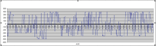
f06-03-9780124104914 — Figure 6.3 ACE profile.

Table 6.5

Comparison of Results from Different SERRegDeployfactor Settings

SERReg Deployfactor	Average ClearedReg (MW)	Average DeployedReg (MW)	Average \|DeployedReg\| (MW)	Average {\|DeployedReg\|/ ClearedReg} (%)	Average ClearedEnergy (MW)	Average SERReg TestScore (%)
0	15.79	−0.999	12.3	78.10%	−0.168	95.16%
0.8	12.88	−0.682	10.01	81.32%	−0.152	99.16%
1	12.23	−0.661	9.53	78.18%	−0.028	100%

t0030

Under SERRegDeployfactor = 1, the score is 100%. But the average cleared regulation is 12.23MW. This result is 61% of the 20 MW capacity. Under SERRegDeployfactor = 0, the score is 95.16%. There are 4.84% of the times that the cleared regulation on SER cannot be counted. If the ACE is in one direction for a long period of time, this number can be larger. The average cleared regulation is 15.79MW. This is 79% of the 20 MW capacity.

In summary, SERRegDeployfactor can be set near zero if the AGC deployment tends to be in both directions for most of the intervals. This can result in more regulation cleared on short-term SERs. However, if the AGC deployment tends to be in one direction for longer periods of time, it is better to set SERRegDeployfactor near one so that the cleared regulation on short-term SERs is available to be deployed. This can result in less regulation to be cleared on short-term SERs.

6 Implementing Performance-based Regulation Compensation

The regulating reserve MCP resulting from the co-optimization is used to pay for the cleared regulating capacity. However, prior to FERC order 755, there was no compensation for the movement of regulation. With the same cleared regulation capacity, fast-ramping resources like short-term SERs can respond to AGC regulation deployment signals more quickly than slower-ramping resources, and tend to provide more movement for regulation. Hence, order No. 755 requires a fair compensation for “the inherently greater amount of frequency regulation service being provided by faster-ramping resources.”

FERC order 755 required each RTO/ISO to use market-based mechanisms to select and compensate frequency regulation resources based on a two-part payment methodology, i.e., a capacity payment to keep the capacity in reserve and performance payments to reflect the amount of work each resource performs in real-time in response to the system operator’s dispatch signal.

In order to meet FERC’s requirement of two-part regulation payment, MISO modified its market rules to require regulating qualified resources to submit two-part regulation offers. The original regulating reserve offer is replaced by a regulating capacity offer (in $/MW/h) and a regulating mileage offer (in $/MW). The regulating capacity offer reflects the cost to hold capacity in reserve and the regulating mileage offer reflects the cost of movement in response to AGC regulation deployment signal.

A new term “regulation mileage” is defined to measure regulation movement. It is the absolute value of up and down movement in MW (mileage) for AGC regulation deployment. The movement for energy or contingency reserve is not counted toward regulating mileage.

Regulating capacity is cleared by the energy and operating reserve co-optimization. Since regulation is deployed on resources with cleared regulating capacity, it is important to incorporate the regulating mileage offer into the clearing process. If only the regulating capacity offer were used in the clearing processes, resources would have an incentive to offer very cheap for regulating capacity so that they could be cleared to provide regulating reserve and very expensive for regulating mileage to get high regulating mileage payment after being deployed by AGC, which would result in very high regulating mileage prices.

In MISO’s implementation, the regulating capacity offer and regulating mileage offer are combined into a single regulating total offer, which is used in the market-clearing processes. In order to combine these two offers, a relationship between regulating mileage and cleared regulating capacity must be determined. The actual ratio between regulating mileage and cleared regulating capacity for the dispatch interval is unknown at the time the regulating capacity is cleared. Hence, MISO calculates a market-wide regulating mileage to regulating capacity ratio based on AGC deployment data and market-clearing results every month. The updated ratio is used in the market-clearing processes for the following month.

Assume the market-wide regulating mileage to cleared regulating capacity ratio for an hour is α, regulating mileage offer is O^RegM($/MW), and regulating capacity offer is O^RegC($/MW/h). The regulation total offer O^RegT($/MW/h) is calculated as:

$\begin{array}{l} O^{RegT} ($ / MW / h) \\ = O^{RegC} ($ / MW / h) + α (/ h) \cdot O^{RegM} ($ / MW) \\ = \{O^{RegC} + α \cdot O^{Re gM}\} ($ / MW / h) \end{array}$ $\begin{array}{l} O^{RegT} ($ / MW / h) \\ = O^{RegC} ($ / MW / h) + α (/ h) \cdot O^{RegM} ($ / MW) \\ = \{O^{RegC} + α \cdot O^{Re gM}\} ($ / MW / h) \end{array}$

si69_e

O^RegT is used as the cost for clearing regulating capacity in the day-ahead and real-time market clearing processes [17]. Essentially, for each MW of regulating capacity cleared in each 5-minute dispatch interval, the cost of deploying (α/12) MW of regulating mileage is incorporated into the clearing processes. As a result, the day-ahead and real-time settlement based on LMP, contingency reserve market clearing price (MCP), and regulating reserve MCP (MCP^RegT) resulting from the co-optimized energy and ancillary service clearing processes will include the cost of deploying (α/12) MW of regulating mileage for each MW of regulating capacity cleared.

When the actual deployed mileage is calculated after the fact, the difference between the regulating mileage target and the regulating mileage considered in the market clearing processes needs to be considered. A regulating mileage MCP (MCP^RegM in $/MW) is calculated as the highest regulating mileage offer from all resources cleared economically for regulating capacity. Assume cleared regulating capacity from the real-time dispatch is R^C (MW) in a 5-minute dispatch interval and the regulating mileage target from AGC for that dispatch interval is R^M. The adjustment to regulating revenue for this dispatch interval is calculated as:

${[R}^{M} - (\frac{α}{12}) R^{C}] \cdot {MCP}^{RegM}$ ${[R}^{M} - (\frac{α}{12}) R^{C}] \cdot {MCP}^{RegM}$

(23)

When the regulating mileage target is more than the regulating mileage considered in the market-clearing process, i.e., $R^{M} > (\frac{α}{12}) R^{C}$ $R^{M} > (\frac{α}{12}) R^{C}$ , MISO pays the additional regulating mileage ${[R}^{M} - (\frac{α}{12}) R^{C}]$ ${[R}^{M} - (\frac{α}{12}) R^{C}]$ at the regulating mileage MCP. Since the regulating mileage MCP is the highest mileage offer from all resources cleared economically for regulating capacity, this part of the payment should always cover the resource’s additional mileage offer cost. When the regulating mileage target is less than the regulating mileage considered in the market clearing process, the undeployed regulating mileage $[(\frac{α}{12}) R^{C} - R^{M}]$ $[(\frac{α}{12}) R^{C} - R^{M}]$ is charged back at the regulating mileage MCP. This may cause a resource to lose profit even if it follows the MISO signal perfectly due to the cross-product opportunity cost between energy, regulating reserve, and contingency reserves and the fact that regulating mileage MCP is the highest regulating mileage offers from all resources cleared economically for regulation. MISO has included an undeployed regulating mileage make whole payment [8] to compensate for any potential profit loss caused by charging back at the regulating mileage MCP.

A performance accuracy measurement is also implemented by comparing the actual outputs of a regulating resource to its corresponding AGC set-point instructions. Regulating payment to a resource is adjusted based on its actual performance.

The market-clearing and settlement changes for FERC order 755 were implemented in December 2012. In the 12 months after the implementation, the following was observed from the production system [16]:

1) MISO’s implementation of regulation mileage is working as designed by providing appropriate regulation compensation based on actual regulation mileage performance. Overall regulation market clearing prices have increased slightly. More regulation capacity is available for substitution for contingency reserves.

2) Overall regulation procurement costs and penalty charges have been relatively steady since the implementation of the regulation mileage enhancement. The net regulation payment to regulating resources in 2013 was $19.9 million, much lower than the payment of $26.1 million in 2012, and mainly driven by regulation performance penalty charges of $11.5 million.

3) Two-part regulation compensation provides fair compensation to fast-ramping resources that can generally provide more and better regulation movement. This compensation method incentivize existing fast-ramping resources to participate in the regulation market, with the benefit of slightly improved operational performance.

a. The actual regulation deployment ratio for faster ramping resources is on average higher than slower ramping resources. It results in more regulation mileage payment to faster ramping resources.

b. The performance of faster ramping resources is better than that of slower ramping resources and hence with less percentage of regulation penalty charges.

c. Regulation has shifted slightly from slower ramping resources to faster ramping resources.

d. CPS1 and BAAL data indicates that system control performance has improved slightly in 2013.

In summary, the implementation of the performance based regulation payment at MISO has met the goal of providing fair compensation to regulating resources based on the actual regulation service provided. Overall, the market has benefited from the performance based compensation mechanism.

By attracting better-performing resources to the regulation market, other traditional resources can free up capacity that is currently held for regulating reserves, and instead, provide energy or contingency reserves. This may potentially reduce the overall cost of the market as well as reduce emissions.

7 Conclusion

This chapter introduced the studies that led to the design to incorporate short-term SERs into the MISO energy and ancillary service market. The physical characteristics of the short-term SER are the best fit for providing regulating reserve. Special constraints are set to avoid regulating reserve cleared on short-term SER to substitute for contingency reserves. Price implications were discussed. The handling of real-time energy dynamics of short-term SERs were then explained. Short-term SERs cannot submit an energy offer to set LMP. Three energy dispatch options were discussed and the option to dispatch energy to allow maximum regulating reserve procurement was adopted. Constraints were implemented to avoid potential negative impacts from the energy dispatch. The implementation in DA and RAC was also discussed. Finally, the relationship between RT-SCED regulating procurement and AGC deployment was analyzed and Monte Carlo simulation results were presented to illustrate the relationship. The enhancement on MISO market rules to comply with FERC order 755 for performance based two-part regulation payment to provide fair compensation to fast ramping resources was also discussed.

..................Content has been hidden....................

You can't read the all page of ebook, please click here login for view all page.

Table of Contents for Chapter 6: Incorporating Short-Term Stored Energy Resource into MISO Energy and Ancillary Service Market and Development of Performance-Based Regulation Payment

Create new playlist

Sign In

Sign Up