
Impact of Energy Storage on Cascade Mitigation in Multi-Energy Systems
Mads R. Almassalkhi*; Ian A. Hiskens† * Assistant professor, School of Engineering, University of Vermont in Burlington, VT.
† Vennema Professor of Engineering, Department of Electrical Engineering and Computer Science, University of Michigan, Ann Arbor, MI.
Abstract
The methods described in this chapter examine a bilevel cascade mitigation scheme that considers both the economic and security objectives in operation of the energy system. The rst level operates on a slow timescale (i.e., hourly) and determines a trajectory of optimal economical set points for generation, storage, load control, and wind curtailment. The second level operates in the background and responds to contingencies (i.e., line outages) on a much faster minute-by-minute timescale to ensure that the system is driven back to a secure and economically optimal operating regime and line overloads are alleviated. The eect of energy storage on the performance of cascade mitigation is investigated through storage scenarios within a multienergyenergy hub" framework. Finally, a temperature-based cascade mitigation is described for the electric bulk power system where the role of energy storage is highlighted with a case-study.
1 Introduction
1.1 Toward the greenfield approach
The National Academy of Engineering named the electric-power grid the greatest engineering achievement of the 20th century [1]. However, as recent large-scale power-grid failures illustrate, the (electro-mechanical) electric grid is being operated closer and closer to its limits. Specifically, the electric grid of the 20th century is aging and congested. Furthermore, it will not be able to meet future demands without operational changes and significant capital investments over the next decades [2]. Thus, the electric grid of the 21st century represents an open problem for the research community and industry. With the development of new technologies, such as, flexible AC transmission devices (FACTS), phasor measurement units (PMUs), renewable and distributed generation, flexible loads, and energy-storage solutions, the tools are available to enable a paradigm shift for the electric grid.
To overcome the limitations of today’s power grid, two main approaches are considered by engineers and scientists. The first approach investigates improvements to energy-delivery systems subject to boundary conditions given by today’s grid structures. The second approach seeks to develop and design a new paradigm for optimal future energy delivery systems, which takes into account novel emerging technologies. By treating the second approach (i.e., the greenfield approach) as the forecasted optimal “target” system, the first approach can be considered a coordinated effort to bridge today’s aging and congested system with the optimal future target system, as Figure 5.1 illustrates.
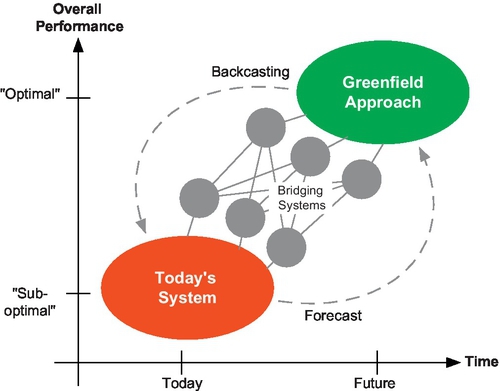
The design and development of the greenfield approach can be considered the long-term goal of power systems engineers and scientists, while the bridging approach can be considered a series of short-term projects. It is within this framework that the work is developed in this chapter. Namely, we build upon the ETH Zürich project “Vision for future energy networks,” which focused on a synergistic interconnected energy systems model as their green-field approach. To accomplish the interconnection of energy systems, the ETH project developed modeling tools such as the “energy hub” and multi-energy carriers and analyzed many scenarios under the new multi-energy context (see [3–5]).
This chapter expands upon the ETH project by applying the “energy-hub” approach to analyze the performance of energy delivery systems with energy storage in contingency scenarios (i.e, line outages). This is achieved by developing a novel model-predictive control (MPC) scheme that ensures efficient operation of energy systems and mitigates the effects of severe line-outage disturbances through feedback algorithms. Developed algorithms are illustrated through numerous simulation studies. The interdisciplinary research presented in this chapter lies at the intersection of power systems, optimization, and controls. Specifically, two model-predictive control-based cascade-mitigation approaches are analyzed herein. The first approach represents a multi-energy approach that considers a simplified system of interconnected natural gas pipelines and electric-transmission systems, which is then developed into a second practical, yet rigorously justified, cascade-mitigation scheme for just the electric bulk-power system.
1.2 Cascade mitigation
Currently, abnormal conditions are handled either through protection operation or operator intervention, depending on the severity of the abnormality. In the latter case, where conditions do not immediately threaten the integrity of plant or loads, operators institute corrective procedures that may include altering generation schedules, adjusting transformer tap positions, and switching capacitors/reactors. For more extreme abnormalities, the protection associated with vulnerable components will operate to ensure they do not suffer damage. This myopic response may, however, weaken the network, exacerbating the conditions experienced by other components. They may subsequently trip, initiating an uncontrolled cascade of outages. This pattern was exhibited during the blackout of the U.S. and Canada in August 2003 [6].
As the amount, type, and distribution of controllable resources increases, operators will find it ever more challenging to determine an appropriate response to unanticipated events. At a minimum, operators will require new tools to guide their decision-making. Given the increased complexity of response actions, a closed-loop feedback process will become indispensable. Furthermore, since power systems are suffused with constraints and limits on states and inputs, model predictive control (MPC) schemes can be particularly useful within the context of contingency management. For a general overview of MPC, see [7–9].
The first application of MPC to emergency control of power systems was [10], where voltage stability was achieved through optimal coordination of load shedding, capacitor switching, and tap-changer operation. A tree-based search method was employed to obtain optimal control actions from discrete switching events. To circumvent tree-based search methods, [11,12] employed trajectory sensitivities to develop MPC strategies. However, those methods focused on voltage stability and did not take into account energy storage nor thermal overloads of transmission lines. Distributed forms of MPC have also been proposed, with mitigation of line-outage cascades considered in [13].
The authors in [14,15] proposed a framework for electrothermal coordination in power systems, and developed temperature-based predictive algorithms that are amenable to energy markets and applicable within existing system controls. Other recent literature, cf. [16,17], focused on model-predictive control of electrical energy systems to alleviate line overloads within a standard DC power flow framework. Specifically, the authors in [17] extended the ideas of [16] to include a linearized current-based thermodynamical model of conductors and an auto-regressive model of the weather conditions (i.e., wind speed and ambient temperature) near transmission lines. This allowed [17] to set a hard upper limit on conductor temperature to ensure control objectives, and allowed MPC to operate the system closer to actual physical limits than if using standard (worst-case weather-based) thermal ratings. Furthermore, [17] illustrated that temperature-based control can outperform current control within a predictive framework.
The cascade-mitigation schemes described in this chapter examine a bi-level cascade-mitigation scheme that considers both the economic and static security objectives in operation of the system. The first level operates on a slow timescale (i.e., hourly) and determines a trajectory of optimal economical set points for generation, storage, load control, and wind curtailment. The second level responds to contingencies (i.e., line outages) on a much faster minute-by-minute timescale to ensure that the system is driven back to a secure operating regime and line overloads are alleviated. The second level does not consider fault conditions and automatic protection schemes, which operate on a sub-second timescale, and assumes transient short-term stability. The effect of energy storage on the performance of cascade mitigation is investigated through storage scenarios within a multi-energy “energy-hub” framework. A temperature-based cascade mitigation is described for the electric bulk-power system where the role of energy storage is highlighted. The work herein represents state of the art in model-predictive cascade mitigation.
1.3 Outline
The chapter is organized as follows. First, basic relevant concepts are described, including line-outage models. Then, relevant system models are introduced and the use of MPC is motivated for cascade mitigation. A bi-level cascade-mitigation scheme that considers economic and security objectives is then discussed. Two cascade-mitigation approaches utilizing model-predictive control (MPC) are discussed: shrinking-horizon and receding-horizon. The former employs a multi-energy “energy-hub” formulation within a simplified shrinking-horizon MPC framework to highlight the role of energy storage and represents a large-scale application of energy hubs within a cascade-mitigation framework. The second approach refines and improves upon the shrinking-horizon MPC scheme and focuses on receding-horizon MPC of electric bulk-power systems with energy storage and analysis of the feedback scheme is provided. The receding-horizon MPC scheme is complemented with a case study of the standard RTS-96 test system augmented with energy storage to highlight the practical, yet rigorously justified, cascade-mitigation scheme.
2 Basic concepts and definitions
To ameliorate possible confusion with terminology, relevant definitions and concepts are described in this section.
2.1 Line tripping
When lines exceed their limits, it is possible that these lines go out of service or trip. The term “line trip” refers to the event that causes a line to go from being in-service to out-of-service. When a line (i, j) is tripped (i.e., out of service) the following must hold:
• no flow (or losses) across (i, j): fij = 0.
• node i and j are decoupled in power flow equations. For example, the DC power flow equation, xij fij = θi – θj, that relates the voltage phase angles of nodes i and j to flow across line (i, j) no longer has to hold.
In general, one of the main goals of a system operator is to ensure that line flows stay within predefined flow limits, which represents a form of network reliability. Therefore, if fij (t) and uij are the (bidirectional) power flow and the power flow rating (i.e., limit) on arc (i, j) at time t, respectively, then, it is desirable to enforce the line flow limit:
|fij(t)|≤uij,
where (i, j) represents arc between nodes i and j. Thus, if system operations satisfy (1) at all times t, arc (i, j) will not be tripped (under normal operating circumstances).
While it is feasible to take inequality (1) into consideration upon determination of an hourly economic energy management schedule, it is unrealistic to expect such a constraint to be valid after the system undergoes a significant disturbance (e.g., multi-line outage). This is due to the fact that flows depend on the physics of the network and cannot be directly guided (e.g., FACTS devices1 are not considered here), which means that the line flows may exceed their limit after a contingency has occurred.
There exists a myriad of approaches to model when an overloaded line should be tripped, ranging from deterministic hard constraints, as in [18], to soft-constrained probabilistic setups described in [19]. This section presents two models of line tripping: one is a simplified deterministic model and the other is probabilistic based on temperature overloads.
2.1.1 Deterministic outage model
The first model employs a simple deterministic outage criterion, which assumes that lines can withstand any power overload for MT minutes before being tripped out of service. That is,
P(line(i,j))tripsattimeMT)={1,iffij(MT)>uij0,else.

This model is obviously conservative, as it will trip lines regardless of the degree of the overload. For example, a 1% overload for 5 minutes is very different from 100% overload for 5 minutes, yet under this simple model both lines would trip. A justification for employing such a simple line-outage model is that sensors may be installed that sample the line flow every MT minutes and trips a line if an overload is sensed. Therefore, under proper control actions, lines should be brought within flow limits by time step MT (assuming synchronization of sensors and actuators). Such controller response aligns with a shrinking-horizon MPC controller which is described in Section 5.1.
2.1.2 Probabilistic thermal outage model
The second model of line tripping is probabilistic and is utilized in Section 6 to more accurately represent the actual line-outage process for electrical transmission systems. For electrical systems, components, such as over-current relays, are often in place to protect the system against abnormal conditions by tripping lines (i.e., taking them out of service). However, these components operate for extreme over-current fault scenarios (e.g., 10,000A) and trigger automatically on a timescale of seconds and mili-seconds and are, therefore, not considered in this work. Instead, the line-tripping behavior of interest in this chapter occurs on a timescale of minutes, which shifts the focus from fault conditions to thermal conditions of transmission lines and sagging. Electrical transmission lines have prescribed power flow limits to prevent dangerous sagging and permanent damage. These limits are related to the thermal capacity of the conductor and the current flowing across the line. The method for calculating the current-temperature relationship of bare overhead transmission lines is described in detail by IEEE Standard 738 [20]. As the temperature of the conductor increases, the thermal expansion causes the line to sag. There is an inverse relationship between the overload on a line and the time it takes before the line sags excessively and must be taken out of service; however, there are no clear rules when a sagging line will be taken out of service (by operator or nature). For example, a human system operator may decide that the red flashing warning sign is sufficiently annoying and trip the line manually or an elephant may just walk into a sufficiently sagging line and cause an outage.2 Excessive line temperature (and resulting sag or possible annealing) may eventuate in line tripping. In short: the higher the temperature, the more likely line tripping becomes. This inverse relationship between conductor temperature and mean time-to-trip (i.e., mean time-to-failure) is captured in the actual system by use of the exponential time-to-failure density parametrized by the temperature overload:
P(line(i,j)tripsattimet)=λ(ΔTij)e−λ(ΔTij)t,
where rate parameter λ (ΔTij) > 0 is a nonlinear function of the temperature overload, defined such that the mean time-to-failure goes to zeros as temperature increases (i.e.,1λ(ΔTij)→0asΔTij→∞)![]() . That is, for each temperature overload, there is different mean time-to-failure. Thus, the probability of line (i, j) tripping during time-interval Ts, given ΔTij, is defined by the cumulative density function (also called the unreliability function):
. That is, for each temperature overload, there is different mean time-to-failure. Thus, the probability of line (i, j) tripping during time-interval Ts, given ΔTij, is defined by the cumulative density function (also called the unreliability function):
P(line(i,j)tripsduringtimek|ΔTij[k])=1−e−λ(ΔTij[k])Ts,
where rate parameter λ(ΔTij[k]) > 0 can be based on the short-time (15-minute) emergency (STE) rating of a transmission line. It has been found experimentally that λ(ΔTij[k]) = (ΔTij[k]/15)6 gives reasonable line-tripping behavior, as shown in Figure 5.2. Notice how the mean time-to-trip decreases with increasing conductor temperature overload.

Furthermore, considering over-current protection on transmission lines (for large overloads), an additional condition can be added to the probabilistic line-tripping model:
P((i,j)tripsatk||facij[k]|uij≥ˉΩ)=1,

where ˉΩ![]() is an upper bound on allowable relative instantaneous overload. For example, if ˉΩ=3,
is an upper bound on allowable relative instantaneous overload. For example, if ˉΩ=3,![]() then a line flow of 300% of nominal thermal limit uij automatically trips line (i, j).
then a line flow of 300% of nominal thermal limit uij automatically trips line (i, j).
With this formulation for line tripping, if a line experiences an overload, the expected time to trip decreases as a function of the inverse of temperature-based rate parameter λ (ΔTij) and sampling time Ts.
2.2 Cascade failures
Given a line-outage model, we can discuss cascade failures. From left to right, Figure 5.3 illustrates three stages of a cascading failure: initial disturbance (left side of figure), cycles of line outages and flow redistributions (center), and a terminal blackout (right). Cascade failures are initiated when a disturbance occurs that forces a redistribution of flows. When a line goes out of service, it can reduce the network’s overall capacity,3 which begets power overloads on the remaining lines as the power flows are redistributed according to Kirchhoff’s laws. If overloads are not alleviated in a timely manner, more lines may go out of service. The cycle of line outages and redistribution of flows, if left uncontrolled, is referred to as a cascade failure. A cascade failure generally terminates in a major blackout, with large areas of a network unable to supply demand.

Furthermore, for electric-power grids, the cascade is multi-scale in a somewhat unusual way. After the initial fault, the first stages of grid failure can proceed relatively slowly, on a scale of hours or minutes. As the cascade develops, the pace of failures can accelerate, with later waves happening on a scale of seconds. Figure 5.4 highlights the accelerating pace of major outage events during the 2003 blackout in the Northeastern U.S. and Canada. Note that the initial two outage events represent transmission lines overheating and sagging into trees. The multi-scale timing of outages has important consequences for any cascade-mitigation strategies. Since longer time scales during the initial cascade allow for significant computations to be performed, it provides an excellent opportunity for feedback control in mitigating the effect of cascading failures. This provides the motivation for the model-predictive control approach developed in later sections.

3 System considerations
The cascade-mitigation schemes proposed herein rely on successive solutions to large optimization problems that drive the system back to a safe and economical operating regime. Large optimization problems generally produce numerical problems for solvers or simply take too long to solve to optimality. Therefore, it is crucial that the cascade-mitigation schemes employ models that are amenable to fast and robust computation. To that effect, we have taken the technical route of employing strictly linear (i.e., convex) models. They are described in the following sections.
3.1 Multi-energy concept: the energy hub
Multi-carrier energy networks may be formulated in different ways. This section will focus the discussion on the “hybrid energy-hub” model initially developed by [25]. Under this formulation, the system operator of an energy-hub network can directly manipulate and control load, generator, and energy-hub (e.g., storage and converter) set points. The energy-hub model is linear, which makes it amenable for computation and optimization. For mathematical details on the energy-hub models, see [26].
Most common energy hubs consist of five simple interconnected elements: inputs, input-side energy storage, energy converters, output-side energy storage, and outputs. To properly describe the flow of power through the energy hub, we need to describe how power flows between these elements. Energy-carrier networks supply power to the hub at the input side, where storage may be available. The energy that was not utilized for storage is dispatched into converters that transform the energy accordingly. On the output side of the hub, converted energy may be utilized for storage or injected into the carrier network connected to that side.
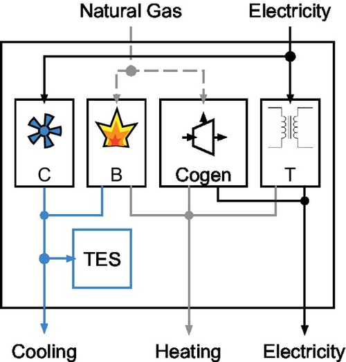
One simple example of an energy hub is shown in Figure 5.5 where a campus energy plant is modeled as an energy hub. The chilled water plant (C), natural-gas steam boiler plant (B), gas turbine cogeneration plant (Cogen), electrical substation (T), and thermal-energy storage (TES) are considered part of the the same energy hub. The supply of electricity and natural gas represent the hub inputs while the outputs are cooling, heating, and electric loads (e.g., buildings and/or processes). The electrical energy is converted to cooling via the chilled water plant and to low-voltage electrical energy by the transformer at relevant efficiencies and injected into the output side. The natural gas consumed at the hub input can be dispatched to the steam boilers (for heating only) or to the Cogen plant where natural gas is converted into both electrical energy and heating. To illustrate the inclusion of storage devices within the energy-hub formulation, consider the chilled water-storage tanks in TES that can store cooling at some charge/discharge efficiency and standby losses. The chilled water plant can store cooling from the electric chillers while the boiler plant can store cooling via absorption processes. The TES can then charge or discharge to achieve objectives related to improved economics (e.g., reduce peak electric consumption) and/or increased reliability (e.g., provide backup when chilled water plant is out of service).
3.2 Energy hubs and cascade mitigation
Hub storage plays a significant role in cascade mitigation since it acts as a “buffer” against disturbances. That is, a system operator can employ stored energy to satisfy temporary energy shortages or overflows, while allowing time for conventional generators to effectively reconfigure their schedules.
Thus, the effectiveness of system operations in minimizing costs and rejecting disturbances depends on the available energy-hub storage infrastructure. Indeed, siting, sizing, and operational capability (e.g., power rating and standing losses) are salient parameters. Siting is important for reducing congestion during peak hours; however, the process for determining optimal location of energy hubs is non-trivial and is not considered here. Instead, this simulation will fix the location of hubs (and storage) within the system and study the effects of varying hub storage capacity and charge/discharge power limits on the cascade-mitigation process.
Under the energy-hub paradigm, we are able to combine multiple types of energy systems and study their combined performance. Therefore, we need to consider multiple types of energy storage, namely, natural gas storage, electrical storage, and thermal storage. Note that, in this work, we consider energy storage to have no standing losses, constant charging and discharging efficiencies4 (see Table 5.1), and we neglect the economics of construction, operation, and maintenance of storage facilities. That is, energy storage represents a cost-free service available to the system operator.
Table 5.1
Summary of different types of energy storage
| Storage | Location | Charge Eff. | Discharge Eff. |
| Natural gas | Only input-side | 99% | 99% |
| Hydrogen | Both sides | 80% | 65% |
| Thermal | Only output-side | 100% | 60% |

3.2.1 Natural gas energy storage
The two main methods used in industry for storing natural gas are “packed” pipelines and underground storage facilities. The packing of pipelines refers to the intended accumulation of natural gas in pipelines by operators. Since such practices are commonly employed for pressure-regulation and only make up a small percentage of natural gas storage capacity, packing of pipelines is not considered in this work. Instead, we consider underground storage in the form of reshaped salt caverns, which have high throughput and can be cycled hourly for both electric and heating loads, and aquifers, which can be regularly withdrawn and have large capacity [27]. The energy hubs that convert natural gas in the proposed multi-energy systems, therefore, contain input-side storage devices that reflect highly efficient underground storage facilities.
3.2.2 Electrical energy storage
With the intermittency of renewable energy (e.g., solar and wind), effective implementation of storage is highly desirable for improving system reliability. Pumped hydro storage and compressed air systems provide two large-scale methods for storing electric-ready power. However, our focus is mainly on distributed storage (e.g., Lithium batteries, fuel cells). Therefore, we consider energy hubs with hydrogen fuel cells that convert to and from electrical energy. Hydrogen storage requires an electrolytic process for charging (i.e., create hydrogen) and employs efficient fuel cells during discharging (i.e., consume hydrogen).
3.2.3 Thermal energy storage
Under the energy-hub paradigm, both natural gas and electrical energy can be converted into thermal energy to satisfy district heating loads. This inherent energy flexibility improves system reliability and by employing thermal energy storage within the hub, we can satisfy distributed thermal loads from stored thermal energy, which reduces network congestion that tends to arise during peak demand. There exists a wide range of thermal energy-storage solutions ranging from molten salt to gas-fired and electric-storage heaters. However, for this work, we will just consider a general form of thermal storage that supplies each heating load. The thermal storage device is employed on the output side of hubs that convert electrical and natural gas energy into heating. We assume a loss-less conversion of natural gas and electrical energy into thermal storage and attribute thermal energy losses to the discharging process.
3.3 Energy-Storage model
The systems considered in this chapter will have energy storage located at various nodes throughout the network. During normal operation of the power system, energy storage plays a significant role in minimizing generation costs from conventional generators, as it allows the system operator to preposition energy in storage during off-peak hours to satisfy demand in the presence of intermittent generation (e.g., wind power) or take advantage of arbitrage. However, during contingency operation, economics become a secondary concern, but energy storage can still play a significant role in cascade mitigation as it acts as a “buffer” against disturbances. That is, a system operator can employ stored energy to satisfy temporary energy shortages or overflows, while allowing time for conventional generators to effectively reconfigure their schedules against ramp-rate limits.
Energy storage is available in many forms (e.g., hydrogen fuel cells, grid-scale battery systems, hydro, gas-filled caverns, thermal energy-storage, molten salts, etc.) and energy-storage devices can be located at various nodes throughout a network. Let n∈ΩEi⊂Q![]() be an energy-storage device at node i, where Q
be an energy-storage device at node i, where Q![]() is the set of storage devices in the system. Assume steady-state storage-power values, a constant slope for ˙En(t)=dEn(t)/dt,
is the set of storage devices in the system. Assume steady-state storage-power values, a constant slope for ˙En(t)=dEn(t)/dt,![]() and treat the storage interface as a conversion process with charging and discharging efficiencies ηc,n and ηd,n, then the relationship between storage state of charge (SOC) and power injected/consumed by device n is:
and treat the storage interface as a conversion process with charging and discharging efficiencies ηc,n and ηd,n, then the relationship between storage state of charge (SOC) and power injected/consumed by device n is:
˙En(t)=dEn(t)dt≈en(t,fQn)×fQn(t).

where the SOC switching mechanism en is defined as:
en(t,fQn)={ηc,n,iffQn(t)≥0(charge/standby)1ηd,n,iffQn(t)<0(discharge).

Since energy-storage devices have two distinct states of operation, charging and discharging, that achieve different efficiencies, energy-storage devices introduce switches in the SOC formulation. The following reformulation of the SOC makes this non-convex nonlinearity more apparent:
˙En(t)=ηc,nfQc,n(t)+1ηd,nfQd,n(t),

fQn(t)=fQc,n(t)+fQd,n(t),
0=fQc,n(t)fQd,n(t),
where the rate-limited charging (c) and discharging variables (d), fQc,n ∈ [0,ˉfQc,n]![]() and fQd,n ∈ [−ˉfQd,n,0],
and fQd,n ∈ [−ˉfQd,n,0],![]() model the switching mechanism explicitly as a complimentarity condition in (8c). The nonlinear complimentarity condition ensures that q can either charge or discharge, but not both simultaneously. To circumvent the nonlinearity, a mixed-integer linear (MIL) formulation can be employed:
model the switching mechanism explicitly as a complimentarity condition in (8c). The nonlinear complimentarity condition ensures that q can either charge or discharge, but not both simultaneously. To circumvent the nonlinearity, a mixed-integer linear (MIL) formulation can be employed:
MIL:fQc,n(t)fQd,n(t)=0⇔{0⩽fQc,n⩽ˉfQc,n(1−zn)−ˉfQd,nzn⩽fQd,n⩽0zn∈{0,1}.

where zn is a binary integer. For example, if zn[k] = 1, then fQc,n[k] ≡ 0 and device n is consequently operating in discharging mode at time step k. While the above linear formulation is equivalent to the nonlinear complimentarity condition, the use of integers is generally not desired, as it greatly increases computational complexity.
To avoid utilizing integers in the linear model, one can ignore the complimentary condition in (8c). This implies that simultaneous charging and discharging is now feasible and is equivalent to a convex relaxation of the original SOC model. Replace (8) with the strictly linear and continuous formulation:
˙En(t)=ηc,nfQc,n(t)+1ηd,nfQd,n(t),
fQn(t)=fQc,n(t)+fQd,n(t).
Employing a forward Euler discretization to (10) with sample time of Ts seconds admits linear continuous first-order discrete SOC dynamics that represents the full linear energy-storage model:
En[k+1]=En[k]+Tsηc,nfQc,n[k]+Tsηd,nfQd,n[k],
fQn[k]=fQc,n[k]+fQd,n[k],
fQc,n[k]∈[0,ˉfQc,n],fQd,n[k]∈[−ˉfQd,n,0].
3.4 Power flows
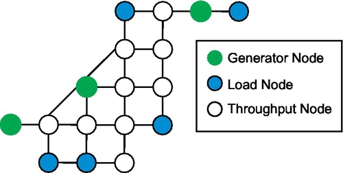
Energy hubs are interconnected via multiple energy-supply networks. The previous section defined how power flows through an energy hub, however, to describe the flow between energy hubs, we need to consider power networks. A power network is a collection of a set of nodes i ∈ N![]() (e.g., buses) and a set of arcs (i, j) ∈ A
(e.g., buses) and a set of arcs (i, j) ∈ A![]() (e.g., transmission lines and gas pipelines) that define a simple graph, as shown in Figure 5.6. The nodes either consume power from the network (i.e., loads), inject power into the network (i.e., generators), or act as throughput nodes that neither inject nor consume power. The sum of power flows into the network (e.g., hub outputs, generators) must equal the sum of flows out of the network (e.g., hub inputs, loads, and losses). In fact, any network must satisfy Kirchhoff’s first law (also called the “power balance”). That is, the net flow into a node must equal the net flow out of the node. Generally, a node may have generators (fGn) and/or loads (fDn) available and, in a system with energy-storage devices, the charging (discharging) corresponds to additional demands (injections) (fQn). Therefore, the power-balance equation is formulated as:
(e.g., transmission lines and gas pipelines) that define a simple graph, as shown in Figure 5.6. The nodes either consume power from the network (i.e., loads), inject power into the network (i.e., generators), or act as throughput nodes that neither inject nor consume power. The sum of power flows into the network (e.g., hub outputs, generators) must equal the sum of flows out of the network (e.g., hub inputs, loads, and losses). In fact, any network must satisfy Kirchhoff’s first law (also called the “power balance”). That is, the net flow into a node must equal the net flow out of the node. Generally, a node may have generators (fGn) and/or loads (fDn) available and, in a system with energy-storage devices, the charging (discharging) corresponds to additional demands (injections) (fQn). Therefore, the power-balance equation is formulated as:
∑n∈ΩDifDn[k]−∑n∈ΩGifGn[k]+∑j∈ΩNiftotalij[k]+∑n∈ΩEifQn[k]=0∀i∈N,
where ftotalij=fij+12flossij![]() is the total flow across line (i,j) and:
is the total flow across line (i,j) and:
• ΩiG – Set of generators at node i (hub outputs and conventional)
• ΩiN – Set of nodes adjacent to node i
• ΩiD – Set of demands (loads and hub inputs) at node i
• ΩiE – Set of energy-storage devices at node i
The power-balance equation in (12) determines the net power generated or consumed at each node. As well as contributing to the power balance, line losses fijloss also drive the temperature dynamics associated with line overloads. This dual role will be carefully studied in Section 6.
Besides interconnecting energy hubs, the main difference between a simple graph and a power network lies with the physics of the particular power flows. That is, there exists a physical relationship between the flow across an arc and the connected nodes. For a simple example, consider an electrical power network and the linear DC flow model:
xijfij=θij,
where xij represents the reactance of arc (i,j), fij is the power flow across said arc, and θij := θi – θj represents the voltage phase angle difference between nodes i and j. In (13), we see that the electrical power flowing across any arc depends on the difference in the phase angle between connected nodes and the reactance of the arc. This physical relationship between nodes and arcs manifests itself differently depending on the nature of the power network model and may be linear (e.g., DC power flow) or nonlinear (e.g., AC power flow). A commonly cited nonlinear power flow constraint is exhibited in natural gas networks, where the flow of natural gas through pipelines depends in a nonlinear manner on the pressure pi at the nodes [28]:
fgasij={kij√pi−pj,ifpi⩾pj−kij√pj−pi,ifpi<pj,
where kij is a constant pertaining to the specific gas and pipeline properties. In addition, power is necessary to maintain pressure at the nodes, which introduces the nonlinear compressor constraints:
fgascom,ij=cijfgasij(pi−pj),
with cij a constant describing the properties of the compressor along arc (i,j).
Regardless of the type of power network, a set of equations describing the appropriate power flow and power balance can be formulated. In this work, the cascade-mitigation schemes employ linear models of power flows (i.e., linearized gas flow and DC power flow). The simulation results will illustrate the value of such simplified models for cascade mitigation.
3.5 Transmission line losses
The probabilistic temperature-based line-outage model described in Section 2.1.2 requires consideration of conductor temperature, which depends on ohmic I2R losses, local ambient conditions (wind speed, insolation), and conductive and radiative conductor heat losses. Thus, to alleviate temperature overloads caused by ohmic heating in transmission lines, it is necessary for a controller to model and manipulate I2R line losses. However, the DC power flow model in (13) ignores active line losses. To establish a relationship for losses on branch (i, j), the AC expression for active power flow across a transmission line can be manipulated to give:
flossij=fij+fji=gij(U2i+U2j−2UiUjcosθij),
where gij,Ui,θij are line’s (i,j) conductance, nodal voltage magnitude, and voltage phase angle difference, respectively. Assuming voltage magnitudes are close to 1.0 pu and approximating cos θij by a second-order Taylor series expansion gives:
flossij≈2gij(1−cosθij)≈gijθ2ij,
⇒flossij≈rijr2ij+x2ijθ2ij≈rijx2ijθ2ij,

where the final step follows because xij ≥ 4rij for most transmission lines. Thus, the “DC” line losses can be written as:
flossij≈rijθ2ijx2ij=rijf2ij,

with the DC flow fij defined in (13). Note that the loss term fijloss is quadratic in θij and is therefore not suitable for a strictly linear constraint formulation.
A computationally amenable model of the quadratic losses can be incorporated into a linear optimization formulation by applying a (piece-wise) linear approximation of losses that circumvents the need for integer optimization (see [29–31]). PWL[fijloss] In fact, you can employ PWL[·] to line losses and develop a strictly (piece-wise) linear model of active line losses in (19) with the following relations:
flossij:=rijx2ijΔθS∑s=1(2s−1)θPWij(s),
S∑s=1θPWij(s)=θ+ij+θ−ij,
θij=θ+ij−θ−ij,
θij∈(−θmax,θmax),
0≤θ+ij,θ−ij,
θPWij(s)∈[0,Δ,θ].
The linear constraint formulation presented in (20) is, in fact, a convex relaxation of the “DC” line losses. Figure 5.7 illustrates the relaxation of PWL line losses. Note that the relaxation given by (20) yields a value for fijloss that is greater than or equal to the piece-wise linear approximation. PWL[fijloss] Equality occurs only when both |θij| ≡ θij+ + θij− and θijPW(s) > 0 ⇒ θijPW(n) = Δθ, ∀ n < s (i.e., adjacency conditions). Under such conditions, the relaxation is considered “tight” and the model is exact with respect to PWL, and the convex relaxation of line losses provides a more accurate method for estimating line losses than standard linearization. When the losses are relaxed (i.e., not tight), overestimated losses are denoted “fictitious losses,” as they exist only as an artifact of the MPC controller model and not in the actual system.

3.6 Model-predictive control
Literature provides two generic approaches for mitigating cascade failures in power networks. The first method predicts disturbances a priori and is based on an off-line computation of all possible or likely failures in the network – the so-called N – k problem, e.g., [32]. With such an approach, control policies are devised to deal with each possible disturbance. A major drawback of this approach is that it does not scale well, since the number of salient contingencies to consider increases exponentially with network size. A second method is based on retroactive control, whereby the uncertainty surrounding the disturbance has been revealed and one can utilize the knowledge available about the disturbance to determine control responses in real-time to mitigate the effects of the disturbance. In the latter approach, the multi-timescale nature of cascading failures provides sufficient time for post-contingency computations. In addition, power/energy systems are suffused with constraints on control inputs and states, which makes model predictive control (MPC) particularly useful in a cascade-mitigation scheme.
MPC is an advanced method of process/batch control that has gained prominence over the last 30 years from its extensive deployment in the chemical industry. For a thorough technical discussion of predictive control in linear systems (see [8]). Basically, MPC provides a method for controlling dynamic systems with constraints on inputs and/or states using tools from optimization. MPC implementations solve on-line, at each sampling instant, a finite-horizon optimal-control problem based on a dynamic model of the plant. Most MPC approaches can be described by the following algorithm:
1. Determine a control sequence that optimizes an objective function over a prediction window, where the measured state at time step k is the initial state.
2. Apply the computed control profile until new process measurements become available.
3. When new measurements are available, set k = k + 1 and repeat step 1.
MPC is most often formulated in the state space by linear discrete-time difference equations. The mathematical formulation is given below.
MPC Formulation The objective of MPC is to drive the system from its current state to some reference state, given by a set point, xsp, in the “best possible” way. In addition, power systems are often modeled with a mix of differential and algebraic states, which beget a set of differential-algebraic equations (i.e., equality constraints). In this work, the constraints are assumed linear (i.e., nonlinear MPC is not discussed) and an l2-norm describes the objective function, therefore, MPC can be formulated as a quadratic programming (QP) problem over a finite prediction horizon5 of length M:
U*[k]=minu[l|k]||x[M|k]−xspk+M||SM+M−1∑l=0L(x[l|k],u[l|k])

s.t.x[l+1|k]=Ax[l|k]+Bu[l|k]+Fz[l|k]
0=ˆAx[l|k]+ˆBu[l|k]+ˆFz[l|k]
Cx[l|k]+Du[l|k]+Gz[l|k]≤d
x[l|k]∈χ,u[l|k]∈U,z[l|k]∈Z
x[M|k]∈Tx
x[0|k]=xmeask,
where x[l|k], u[l|k], and z[l|k] represent the dynamic state, control input, and algebraic state variables, respectively, at predicted time 0 ≤ l < M, given initial measured state xmeask![]() at time k. The optimizer,
at time k. The optimizer,
U*[k]={u*[0|k],u*[1|k],…,u*[M−1|k]},
represents the open-loop optimal control sequence over the prediction horizon at time k. The appropriately-sized matrices A,B,F and Â,ˆB,ˆF,C,D,G![]() describe dynamic and algebraic constraints, respectively. The objective function in (21a) is defined by:
describe dynamic and algebraic constraints, respectively. The objective function in (21a) is defined by:
L(x[l|k],u[l|k])=||x[l|k]−xspk+l||Q+||u[l|k]−uspk+l||R,
where xspk+l![]() and uk + lsp refer to a reference trajectory at time k + l, the norms are defined by ||y||B ≡ yTBy, and weighting matrices SM≻¯
and uk + lsp refer to a reference trajectory at time k + l, the norms are defined by ||y||B ≡ yTBy, and weighting matrices SM≻¯![]() 0 and Q≻¯
0 and Q≻¯![]() 0 are non-negative definite while R
0 are non-negative definite while R ![]() 0 is positive definite. Expressions (21b) and (21c) describe the differential-algebraic (DAE) dynamics. Expressions (21d), (21e), and (21f) define static inequality constraints, bounds on states and inputs, and a terminal state constraint set, respectively. Equation (21g) establishes the initial state for MPC.
0 is positive definite. Expressions (21b) and (21c) describe the differential-algebraic (DAE) dynamics. Expressions (21d), (21e), and (21f) define static inequality constraints, bounds on states and inputs, and a terminal state constraint set, respectively. Equation (21g) establishes the initial state for MPC.
In this chapter, two specific MPC techniques are employed: shrinking-horizon and receding-horizon MPC. These two approaches are described in detail within the context of cascade mitigation in Sections 5 and 6, respectively.
4 Bi-level cascade-mitigation framework
Economic dispatch problems allow computation of economically optimal trajectories, which the system operator tracks via available generation, forecasted load, and other available control actions. However, if a significant disturbance takes place, the operator must modify his economical trajectory to prevent overloads and subsequent line outages. This requires the formulation of a contingency (safety) controller, which responds quickly to a disturbance and drives the system back to a secure and economical state, from which economic dispatch can be re-initiated and normal (economic) operation can resume. Since economic and security objectives are often competing objectives, it is natural to form two separate controllers for each task. Therefore, a bi-level hierarchical control strategy is employed. Figure 5.8 illustrates the proposed bi-level operation of the system.
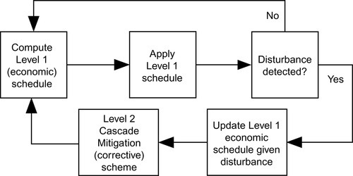
The “Level 1” controller is enlisted to compute an economically optimal schedule for each hour of the day. When a disturbance takes place (e.g., line outage), Level 1 provides an economic reference for the “Level 2” contingency controller, which shifts operation from economically optimal (e.g., hourly) to corrective (e.g., minute-by-minute) in order to alleviate line overloads. When Level 2 signals that the system is secure, economic operation resumes with Level 1. The Level 2 cascade-mitigation controller is formulated as an MPC problem.
4.1 Level 1: economically optimal energy schedule
Over a 24-hour period, Level 1 computes an optimal energy schedule that determines how to best operate energy storage, conventional generation, flexible loads, and available renewable energy based on forecasts. The Level 1 schedule is, therefore, similar to standard economic dispatch [33], except that the temporal coupling introduced by energy storage implies optimization over a horizon rather than a single time step. In addition, any quadratic line losses can be included with a standard piece-wise linear (PWL) DC approximation as presented in [29].
The Level 1 model enforces line-flow limits to ensure that, under accurate model and forecast scenarios, no lines are overloaded (i.e., the system is “safe” and economical). The dispatch schedule is computed as a multi-period quadratic programming (QP) problem whose objective is to minimize energy (fuel) costs of conventional generators:
Cost(fGn[k])=an(fGn[k])2+bnfGn[k],
where an [$/h-pu2] and bn[$/h-pu] are constant parameters for generator n and fGn[k] is its output power at time step k.
The Level 1 schedule establishes a reference signal over a multi-hour horizon, consisting of the economically optimal system set points xsp, and the operator control actions usp required to achieve those optimal set points. The schedule is submitted to the operator and recomputed every hour. For details on Level 1 formulation, see [22,26].
4.2 Level 2: corrective controller
The Level 2 controller operates in the background to track the reference trajectories computed from Level 1 (i.e., the economic set-point values). The corrective controller employs a linear model of the actual system and operates on a minute-by-minute timescale.6 If a disturbance takes place (e.g., a line outage), Level 2 computes corrective control actions u[k] in a MPC fashion that steers the system towards a safe and economically optimal state as provided by a Level 1 reference.
Level 2 considers ramp-rate limits on conventional generators, dynamics and power ratings of grid storage devices, and can incorporate the thermal response of overloaded lines. Note that, in Level 2, lines are no longer subject to a hard flow limit constraint and, instead, the controller seeks to drive overloaded lines below respective limits. The Level 2 MPC-based cascade-mitigation scheme is formulated as a quadratic programming problem (QP) over a finite prediction horizon M.
The Level 2 cascade mitigation discussed in Section 5 employs a shrinking-horizon (i.e., M → 0) MPC-based scheme within a simplified framework of energy hubs. In Section 6, receding-horizon MPC (i.e., M fixed) is described for a temperature-based cascade-mitigation scheme within a bulk electric-power system setting.
5 Multi-energy cascade mitigation
This section investigates how the presence of conversion and storage processes and technologies in a multi-energy system setting helps mitigate the effects of large network disturbances (i.e., line outages) and halts cascade failures.
Our initial work in the area of cascade mitigation proposes a low-level MPC-based controller that only is allowed to shed load in the final control instance. Once a disturbance is detected by the system monitor, operation of the system is switched from an hourly economic schedule to a fast timescale MPC scheme (one-minute time steps). During the fast timescale, nominal load and intermittent power injections are fixed at their most recent slow timescale values, and generation and storage-energy delivery rates are taken into account.
5.1 Shrinking-horizon MPC (SHMPC)
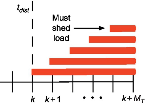
In this MPC-based cascade-mitigation scheme, if lines are overloaded after MT minutes, they automatically trip (i.e., a sensor may measure overloads every MT minutes and trip lines based on simple overload criteria). That is, a deterministic line-tripping model is employed in the multi-energy setting. Therefore, it is sensible to utilize a prediction horizon of MT minutes and assume new measurements are available every minute (and that computation of open-loop control sequences is instantaneous). Furthermore, in attempting to halt the cascade, load-shedding is only allowed in the final time step MT, as a last resort to bring line flows within their limits. Accordingly, there is no reason for our prediction window to extend beyond minute MT and, therefore, the prediction window shrinks by one minute after every measurement update. This method of MPC is often referred to as “fixed-point” or “shrinking-horizon” MPC (SHMPC) [34]. SHMPC considers a prediction horizon that is fixed in time as illustrated in Figure 5.9.
Consider an energy system at time k over M = MT minutes (i.e., initial prediction horizon) with sample time Ts = 1 minute. Then, the SHMPC algorithm is given by:
Shrinking-Horizon MPC Algorithm:
1. Given initial state x[k], solving an optimal control problem over horizon [k, k + M] yields the open-loop control sequence {u[l|k]}l = 0M − 1.
2. For time [k, k + 1), apply the first instance of control sequence u[0|k] to the system with a zero-order hold.
3. Measure new system states x[k + 1], set k := k + 1.
4. Set M : = M – 1 and, if M > 0, repeat step (1). Else, STOP.
As can be realized from the above SHMPC process, with each successive control action, the horizon shrinks by 1 minute until horizon has length 0. At the end of the horizon some physical process may have reached a critical juncture, such as presented with the simple deterministic line tripping model: lines may trip.
If the MPC model has no errors and matches the real system, no overloads will remain at time k + MT, and the cascade will be halted. On the other hand, if the MPC model is imperfect, some overloads may remain. If more lines do trip, one would re-run SHMPC with redrawn horizon M = MT and this shrinking/redrawing horizon cycle continues until SHMPC relieves all line overloads. At that point, the slow-timescale Level 1 is updated with a new post-disturbance network topology, and the latest values for generation, storage and load, and the optimal schedule over the remainder of the 24-hour period are determined. An overview of the energy-hub system operation under closed-loop control is illustrated in Figure 5.8. The cascade-mitigation scheme interfaces with the “real system” as well but on a faster timescale. Note that without the look-ahead feature of MPC, a closed-loop controller acting only at minute k + MT would shed more load, as it would not be able to properly allocate storage utilization to overcome possible future generator power limits.
To contrast the performance of the shrinking-horizon MPC scheme, we consider the base case of a “dumb” controller. The “dumb” controller seeks only to satisfy demand (i.e., avoid load shedding) and line flows are given by the power flow solution with no regard for line flow limits. Therefore, the “dumb” controller will be unlikely to alleviate overload and undergo significant cascading failures.
5.2 Linear SHMPC model outline
The energy-hub model from [26] is employed in the SHMPC scheme, which is detailed in [22] and outlined below.
5.2.1 Objective function
The objective of the SHMPC (i.e., Level 2) is to alleviate all line overloads by minute MT and shed minimal load in the process. To minimize load shedding, rescheduling of energy-storage utilization and generation is possible. Energy conversion and storage represents cheap control while generators are reconfigured based on their cost-curves (i.e., expensive generation is expensive to ramp up and down). A small penalty is placed on wind curtailment while a large penalty is placed on load control.
5.2.2 Constraints
• linear DC power flow model for each electric-transmission line;
• linearized natural gas flow model for each pipeline (see (14),(15));
• linear energy-hub flow equations for each hub;
• mixed-integer linear energy-storage SOC integrator dynamics;
• limits on network elements (e.g., storage, renewable and conventional generation, loads);
• ramp-rate limits on conventional generators; and
• load control is only allowed at the end of the horizon (i.e., last control instance), which is the instance after which line flow limits must be satisfied to avoid line tripping.
5.2.3 Base case
For the base case, the arc flows are given by the power-flow solution with no regard for flow limits. Thus, the base-case problem may undergo significant cascading failures and represents a controller with no information about the disturbance or line overloads. The goal of this “dumb” controller is, therefore, to just satisfy the load.
5.3 Simulations of SHMPC-based cascade mitigation
The formulation of energy hubs described in [26] permits the construction of arbitrarily large interconnected energy-hub networks. In this section, the effects of disturbances (i.e., line outages) under different energy-storage scenarios for small and large energy-hub systems are investigated with simulations. Because current power-grid operating and planning standards ensure power systems are in a reliable condition even if one contingency occurs (i.e., N – 1), the initial disturbances will consist of multiple simultaneous line outages. Each system consists of an electrical network, a natural gas network, district heat loads, wind turbines, and multiple energy hubs that couple the four different energy types.7 The smaller system is useful in describing how the SHMPC approach mitigates a cascade failure, while the larger system allows us to better showcase the cascading effects and role of mitigation.
Employing the SHMPC cascade-mitigation scheme, the following simulations investigate the performance of the scheme under different energy-storage scenarios. That is, simulations are used to investigate how the availability (i.e., capacity) and performance (i.e., charge/discharge power limits) of energy-storage devices impact the level of load control.
The random grid-generating techniques proposed in [35] are employed again to construct two multi-energy systems – a small 11-hub system and a larger 69-hub system and subject each to a multi-line outage. The small energy-hub system is shown in Figure 5.10. Due to the size of electrical and natural gas networks and the random interconnectivity with energy hubs, a meaningful visualization of the larger energy-hub system is not clear and is excluded here. The smaller, simpler system enables a clear understanding of how storage is utilized to mitigate cascade failure, whereas the larger system becomes useful in the discussion as it exhibits meaningful cascade behavior.

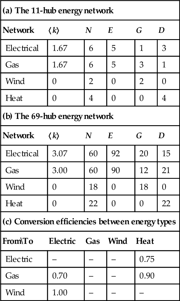
The topological characteristics of the two systems are given in Tables 5.2a and 5.2b where N, E, G, and D represents the number of nodes, lines, generators, and loads for each network, respectively. There are 11 energy hubs in the small system and 69 energy hubs in the large system to couple the four different energy networks. The energy conversion efficiencies are given in Table 5.2c. All hubs connecting the wind network to the electrical network have output storage, while applicable input and output hub storage is added randomly to all of the remaining hubs.
Table 5.2
Randomly generated network characteristics
| (a) The 11-hub energy network | |||||
| Network | 〈k〉 | N | E | G | D |
| Electrical | 1.67 | 6 | 5 | 1 | 3 |
| Gas | 1.67 | 6 | 5 | 3 | 1 |
| Wind | 0 | 2 | 0 | 2 | 0 |
| Heat | 0 | 4 | 0 | 0 | 4 |
| (b) The 69-hub energy network | |||||
| Network | 〈k〉 | N | E | G | D |
| Electrical | 3.07 | 60 | 92 | 20 | 15 |
| Gas | 3.00 | 60 | 90 | 12 | 21 |
| Wind | 0 | 18 | 0 | 18 | 0 |
| Heat | 0 | 22 | 0 | 0 | 22 |
| (c) Conversion efficiencies between energy types | |||||
| FromTo | Electric | Gas | Wind | Heat | |
| Electric | – | – | – | 0.75 | |
| Gas | 0.70 | – | – | 0.90 | |
| Wind | 1.00 | – | – | – | |
The energy-storage scenarios are considered by varying storage capacity and storage power limits from the nominal values by a given factor. For example, for scenario (capacity, power) = (0.25, 0.10), energy-storage capacity is at 25% of nominal and power limits are 10% of nominal. The idea is to compare the effect of different energy-storage scenarios on the average load shed over the 24-hour period. In particular, the scenarios include systems with “no” (0), “some” (≈ 0.25), “nominal” (1.0), and “a lot” (10) of storage capacity, while the system storage devices are subject to “small” (0.10), “nominal” (1.0), and “large” (5 ≥) power limits.
• Small 11-hub system:
In the nominal (1,1) SHMPC case, the 11-hub system from Figure 5.10 undergoes a disturbance that results in the outage of lines 2,5, and 8. The loss of the three lines leaves line 9 (natural gas) with a significant overload, which must be cleared to avoid tripping the line. Under the SHMPC scheme, generators are reconfigured (considering power limits), storage is utilized, and minimal load is shed over the 5-minute interval to avoid tripping line 9. The Level 1 schedule is updated to reflect the multi-line outage and some load (≈ 20%) must be shed until wind power becomes available towards the end of the day. In the nominal base case with the “dumb” controller, line 9 is not protected and trips after 5 minutes, which leaves the system in a weak state and results in heavy load-shedding (≈ 50%).
The results of the 11-hub system are shown in Tables 5.3 and 5.4 Increasing storage capacity generally reduces the amount of load shed and improves performance of cascade mitigation, which is expected, since more energy can be stored and is available to inject into the system upon the disturbance. However, the general trend suggests that lowering power limits improves performance. The reason behind this trend is that the MPC scheme does not care about the state of the system beyond the halting of the cascade and will maximally utilize (free) stored energy to satisfy demand and avoid shedding load. However, with small power limits, the amount of stored energy is effectively rationed during the cascade-mitigation process and some conventional generation is needed to satisfy demand and halt the cascade. This balance between generation and energy utilization allows MPC to halt the cascade and best positions the multi-energy system to satisfy load demand over the subsequent period (following the cascade).
In the base case, the amount of load shed under scenario (10, 5.0) is relatively low, because line 9 is “accidentally” not overloaded at minute 5. The term “accidentally” is used here since the base-case controller attempts to satisfy all demand at the lowest cost with no regard for flow limits. Furthermore, for the (10, 5.0) scenario, the base case sheds marginally less load than the MPC scheme over the 24-hour period. This is because the optimization does not penalize the spilling of wind power, which means that the MPC scheme can use available energy storage and wind power at the same cost. Thus, stored energy in the future (i.e., beyond the 5-minute prediction window) has no value to the MPC controller. MPC employs available energy storage and spills wind power, while the base case utilizes available wind power. The MPC response is optimal over the 5-minute period, but with the cascade halted, it leaves the system with less energy stored. This results in a marginal increase in load-shedding over the remaining hours.
Table 5.3
MPC energy scenario results for 11-hub system
| Avg. load shed (%) | Capacity | ||||
| 0 | 0.25 | 1.0 | 10 | ||
| 0.10 | 12.7 | 10.6 | 9.1 | 8.7 | |
| Power | 1.0 | 12.7 | 10.8 | 9.0 | 9.2 |
| 5.0 | 12.7 | 10.8 | 10.6 | 10.6 | |
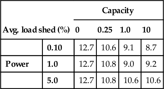
Table 5.4
Base case energy scenario results for 11-hub system
| Avg. load shed (%) | Capacity | ||||
| 0 | 0.25 | 1.0 | 10 | ||
| 0.10 | 32.3 | 30.6 | 28.9 | 28.5 | |
| Power | 1.0 | 32.3 | 32.3 | 30.1 | 29.8 |
| 5.0 | 32.3 | 32.3 | 31.9 | 10.4 | |
• Large 69-hub system:
The trends from the 11-hub system apply to the 69-hub system as well, and the results are provided in Tables 5.5 and 5.6. As storage capacity increases and power limits decrease, the performance of MPC increases for the same reasons mentioned above.
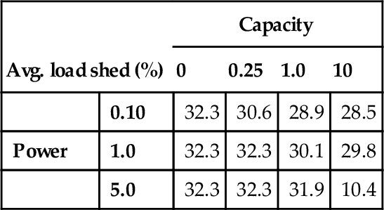
In the base case, the trend is not as strong, but nonetheless discernible. While the complexity of the network obfuscates the subtleties of the result, it is worth noting that for the scenario without storage (i.e., zero capacity), the amount of load shed is similar to low- and medium-capacity scenarios (0.2, *) and (1.0, *).
The behavior of both the base-case system and the MPC cascade-mitigation scheme are depicted in Figures 5.11 and 5.12, for energy scenarios (0, 10), (0.20, 10), (1.0, 10), and (10,10). (Note that thicker lines represent higher capacity scenarios.) In fact, for scenarios (*, 10), the base-case system generally sheds more and more load as storage capacity increases. This is because the base case is uncontrollable in the sense that it does not regard line-flow limits and, for larger systems, this results in significant line tripping as seen in Figure 5.11a. At high power limits and with increasing storage capacity, the base-case controller will inject more stored energy into the system (Figure 5.11c) which, coupled with non-trivial generation levels (Figure 5.12), results in line tripping (Figure 5.11a) and fragmentation of the system. The fragmentation leads renewables to become isolated from loads, which is evident in the base case in Figure 5.11b, since the increase in available wind power (in evening and at night) is unable to recover shed load. The fragmentation is most severe in the highest capacity case, where available wind power is separated from loads and can only be utilized to aimlessly increase energy-storage levels.
Table 5.5
MPC energy scenario results for 69-hub system
| Avg. load shed (%) | Capacity | ||||
| 0 | 0.20 | 1.0 | 10 | ||
| 0.10 | 1.1 | 0.9 | 0.5 | 0.4 | |
| Power | 1.0 | 1.1 | 1.0 | 0.7 | 0.5 |
| 10 | 1.1 | 1.0 | 0.7 | 0.7 | |

Table 5.6
Base-case energy scenario results for 69-hub system
| Avg. load shed (%) | Capacity | ||||
| 0 | 0.20 | 1.0 | 10 | ||
| 0.10 | 23.8 | 24.7 | 23.7 | 19.9 | |
| Power | 1.0 | 23.8 | 23.1 | 23.7 | 14.9 |
| 10 | 23.8 | 23.1 | 24.8 | 29.4 | |


Note that “No Disturbance” cases represent economically optimal energy management without any line outages. However, in the absence of a disturbance, there is still a need to shed some nominal load when wind power reaches its nadir and no more power can be injected by conventional generation without exceeding flow limits. This is a remnant of the fact that the random networks generated do not properly capture the design and planning of real transmission power networks.
Furthermore, it is worth noticing that the zero-capacity MPC scheme (0, *) sheds only 1.1% of total load while the optimal MPC storage configuration (10, 0.1) sheds 0.4% of total load. Therefore, one should ask if the investment made in storage devices is worth the marginally improved cascade-mitigation performance (a 0.7% reduction in load shed). Indeed, with the base-case minimal load shed of 14.9%, the MPC scheme without storage may provide a sufficient cascade-mitigation solution. However, other factors, such as intermittency and congestion reduction, suggests the need for considering energy-storage devices in the investment process.
6 Cascade mitigation in electric-power systems
Despite the simple energy-hub SHMPC formulation and the crude deterministic line overload model, the scheme discussed in Section 5 provided valuable insight into the role of energy storage for cascade-mitigation purposes and motivated the use of model-predictive control. In addition, while the coupling of energy infrastructures may provide an opportunity to improve upon network resilience and protect against cascade failure, investigations into the natural-gas operations show that natural-gas systems are significantly different from electric-power systems. Namely, there is a timescale separation between the two power systems, with electricity flowing at nearly the speed of light while natural gas pipelines experience gas flows of up to 60 miles per hour (around 100 km/hr). This relatively slow rate of energy flowing in natural gas systems gives rise to a different role for the transmission pipeline system. Specifically, natural-gas transmission systems operate by filling, on a seasonal timescale, large underground natural-gas storage facilities near power and heating-load distribution centers. Under such physical circumstances, the notion of cascade failure in natural gas systems becomes less interesting due to timescale separation between electric and natural gas networks. As a result, the focus in this section shifts from multi-energy system models to cascade-mitigation in bulk electric-power systems where it will be shown how energy storage can be utilized to actively alleviate line overloads. In addition, the flow-based SHMPC formulation is replaced by a more robust temperature-based formulation in the form of receding-horizon MPC. Finally, a novel energy-storage algorithm is introduced that takes advantage of the feedback inherent to MPC to overcome common challenges associated with predictive optimization of standard energy-storage models.
6.1 Receding-Horizon MPC
The SHMPC approach suffers from two major drawbacks:
• An unpredicted event could take place towards the end of the shrinking-horizon period, which leaves the system unable to recover in the remaining time.
• As the horizon shrinks and approaches the final time, the control law typically “gives up trying” since there is too little time to go to achieve anything useful in terms of objective function reduction.
The above two shortcomings surrounding SHMPC can be overcome with the notion of receding-horizon MPC, which considers a prediction horizon that does not shrink but, instead, remains fixed in length and moves with time. This makes receding-horizon MPC immune against the above above drawbacks and, therefore, offers a more robust control paradigm than SHMPC. That is, consider a system with a prediction horizon of MT minutes and sample time Ts = 1 minute and assume the initial time step is k, then the receding-horizon MPC is summarized by the following algorithm.
Receding-horizon MPC algorithm:
1. Given x[0|k] := x[k], solve an optimal control problem over horizon [k, k + MT] to retrieve an open-loop control sequence {u[l|k]}MT−1l=0![]() .
.
2. Apply the first instance of control sequence to the system: u[k] := u[0|k].
3. Measure the new system state x[k + 1] := f (x[k],u[k]).
4. Set k = k + 1 and repeat step (1).
As the above MPC process illustrates, with each successive control action, the horizon recedes, as the name implies. Note that in this work, the prediction and control horizons are assumed equal to MT.
The Level 2 model for the receding-horizon MPC cascade-mitigation scheme is similar to the SHMPC scheme, where we considered ramp-rate limits on conventional generators and the dynamics and power limits of grid-storage devices. However, with the temperature-based cascade-mitigation scheme, receding-horizon MPC also incorporates the thermal response of overloaded lines. Note that in Level 2, lines are no longer subject to a hard flow-limit constraint. Rather, the controller seeks to drive conductor temperatures below their respective limits. Note that the receding-horizon MPC optimization is still formulated over a finite prediction horizon as described in (21).
The details of the Level 2 receding-horizon MPC model, system states, and controls are developed and discussed in [31]; however, for sake of completeness, a summary of the model is provided below. The states and inputs associated with the proposed formulation of an MPC cascade-mitigation scheme for an electric-power system are outlined here.
Dynamic states (x): there are three types of dynamic states:
• ΔˆTij,![]() line (i, j) conductor temperature overload w.r.t. limit Tijlim.
line (i, j) conductor temperature overload w.r.t. limit Tijlim.
• En, state of charge (SOC) for energy-storage (ES) device n.
• fGn, power output level for generator n.
Control inputs (u): the formulation employs five types of control inputs:
• ΔfGn, change to conventional generator n output level.
• fspillGWn,![]() wind spilled from nominal, for wind turbine n.
wind spilled from nominal, for wind turbine n.
• fDnred, demand response (reduction) from nominal, for load n.
• fQc,n , fQd,n, charge (c) and discharge (d) rates for ES n.
Uncontrollable inputs: there are three types of forecast (uncontrollable) inputs (i.e., exogenous disturbances):
• fDnnom, nominal available power from wind turbine n.
• fDnnom, nominal demand, for load n.
• dij, ambient temperature and solar gain, for line (i, j).
Algebraic states (z): models require nine types of algebraic states:
• fij, real power flowing through line (i, j).
• fijloss real power losses for line (i, j).
• θij, phase-angle difference between nodes i and j.
• θij+, θij−, absolute value approximation of |θij |.
• {θijPW(s)}s = 1SS-segment PWL approximation of |θij|2.
• fGWn,![]() real power injected by wind turbine n.
real power injected by wind turbine n.
• fDn, real power consumed by load n.
• fQn, total power injected or consumed by ES n.
From the above descriptions, state and input vectors are defined by:
x=col{ΔˆT,E,fG},
u=col{ΔfG,fspillGW,fredD,fQc,fQd,ψ},
z=col{θ,θ+,θ−,θPW,f,floss,fD,fGW,fQ}.
6.1.1 MPC objective function
The objective of the MPC scheme is to determine the optimal control actions that alleviate temperature overloads, ΔˆTij,![]() while minimizing deviations from the economic set points established by Level 1. Accordingly, the MPC objective function is composed of the terms:
while minimizing deviations from the economic set points established by Level 1. Accordingly, the MPC objective function is composed of the terms:
po(ΔˆTij[l])2-linetemperatureoverload
![]()
pg(fGn[l]−fSPGn,k+l)2-deviationfromreferencesetpoint
![]()
pr(ΔfGn[l]−ΔfSPGn,k+l)2-changesingenerationramping
![]()
pe(En[l]−ESPn,k+l)2-deviationfromreferenceSOC
![]()
pq(Qn[l]−QSPn,k+l)2-changesinreferencedis/charging
![]()
ps(fshedDd[l])2-loadcontrol
![]()
pw(fspillG,wind[l])2-windcurtailment
![]()
where reference values, denoted (·)sp, refer to the economically optimal set points computed in Level 1.
Based on the state and input definitions in (25), the following weighting matrices define the objectives of the MPC scheme:
Q=diag{poI,pe10M2I,pg10M2I}≻0,
SM=diag{poI,peI,pgI}≻0,
R=diag{prI,pwI,psI,pqI,pqI}≻0,
where I represents the identity matrices of appropriate dimensions, po > 0 are weighting coefficients for states and inputs, and diag{·} denotes a block-diagonal matrix. Note that the terminal cost matrix SM is designed to penalize deviations from economical references for storage SOC and conventional generation states more severely than does the weighting matrix Q. This is because MPC does not care how these reference signals are tracked, only that they are being considered at the end of the horizon. The weighting matrices are employed in (27a).
6.1.2 Electric-system constraints
For each time k, the dynamic states xmeask![]() are measured and represent the initial state of the MPC system model. Then, the full MPC formulation is defined as a quadratic programming (QP) problem:
are measured and represent the initial state of the MPC system model. Then, the full MPC formulation is defined as a quadratic programming (QP) problem:
minu[l]||x[M]−xspk+M||SM+M−1∑l=0L(x[l],u[l])

ΔTij[l+1]=τijΔTij[l]+ρijΔflossij[l]+δijΔdij,
En[l+1]=En[l]+Tsηc,nfQc,n[l]−Tsηd,nfQd,n[l],
fGn[l+1]=fGn[l]+ΔfGn[l],
ΔˆTij[l]=max{ΔTij[l],0},
0=fQc,n[l]fQd,n[l],
0=x2ijflossij[l]−ΔθS∑s=1(2s−1)θPWij(s)[l],
0=θ+ij[l]+θ−ij[l]−S∑s=1θPWij(s)[l],
0=θ+ij[l]−θ−ij[l]−θij[l],
0=Γi(fij[l],floss,estij,k,fGn[l],fDn[l],fQn[l],fGWn[l]),
0=xijfij[l]−θij[l],
fDn[l]=fnomDn[l]−fredDn[l],
fQn[l]=fQc,n[l]−fQd,n[l],
fGWn[l]=fnomGWn[l]−fspillGWn[l],
x[l]∈χ,u[l]∈U,z[l]∈Z,
x[M]∈Tx,
x[0]=xmeask,
for all l ∈ {0,1,..., M-1} = M![]() , where x[l], u[l], and z[l] represent the dynamic state, control input, and algebraic state variables, respectively, at predicted time k + l given initial measured state at time k,. xmeask
, where x[l], u[l], and z[l] represent the dynamic state, control input, and algebraic state variables, respectively, at predicted time k + l given initial measured state at time k,. xmeask![]() This notation has been adopted for clarity of presentation. The more precise forms, x[l|k], u[l|k], and z[l|k], appear in [31]. The objective function (27a) was described in the last section and is defined by (23).
This notation has been adopted for clarity of presentation. The more precise forms, x[l|k], u[l|k], and z[l|k], appear in [31]. The objective function (27a) was described in the last section and is defined by (23).
Expressions (27b), (27c), and (27d) represent the linear (discrete time) dynamics associated with conductor temperature for line (i,j), SOC for energy-storage device n, and the power supplied by generator n, respectively. The thermal conductor model is based on the IEEE standard describing the temperature-current relationship in overhead conductors [20]. Temperature dynamics in (27b) are linearized with respect to the conductor temperature (Tijlim[°C]) obtained for steady-state ampacity (Iijlim[A]) and conservative ambient parameters. Accordingly, ΔTij = Tij–Tijlim and, Δfijloss = fijlossSb/3Lij − Rij(Iijlim)2 where Sb [VA] and Lij [m] are the three-phase per-unit power base and conductor length, respectively, and Rij [Ω/m] is the resistance per unit length. Also, Δdij = dij – dij* describes deviations from representative exogenous conditions, ambient temperature Tamb*, and solar heat gain rate qs*, with qs a function of conductor diameter and solar conditions. However, it has been assumed for these studies that ambient temperature and solar heat gain rates remain fixed over the period of interest (i.e., Δdij = 0).
Constraint (27e) enables the main objective of alleviating temperature overloads while not incentivizing under-loading of lines. That is, MPC should compute control actions that only consider lines with ΔTij[l] > 0. Keeping in mind the QP formulation, the implementation of this temperature objective can be relaxed to the linear formulation:
0≤ΔˆTij[l],
ΔTij[l]≤ΔˆTij[l].
Because the objective function penalizes ΔˆTij![]() , this relaxation will always be tight.
, this relaxation will always be tight.
The complementarity condition (27f) ensures that energy-storage devices cannot simultaneously charge and discharge. Since exact (integer-based) implementation of complementarity would considerably increase computational complexity of the proposed scheme, the algorithm described in Section 6.1.4 has been adopted for (approximately) enforcing (27f).
A convex piece-wise linear (PWL) approximation of line losses is described by algebraic relations (27g), (27h), and (27i). This PWL relaxation utilizes S segments of width Δθ = θmax/S and is modeled using the algebraic states θij+, θij−, {θijPW(s)}s = 1S In [31], it was proven that if a line experiences a temperature overload at predicted time l + 1, then for all prior time steps (i.e., k ≤ l) the convex relaxation will be exact with respect to PWL approximation. When the relaxation is locally tight, the controller has a meaningful and relatively accurate model of line losses, and hence of line temperature. This allows MPC to compute control actions that relieve line overloads.
Equations (27j) and (27k) denote nodal power-balance constraints (∀i∈N)![]() and DC power flows, respectively. Power balance is implied by Kirchhoff’s law: power flowing into node i must equal the power flowing out plus/minus that injected/consumed. Note that the term fij,kloss,est in (27j) is a constant estimate of line losses at time step k. It is shown in [31] that by decoupling this loss term from fijloss, the PWL relaxation inherits crucial tightness properties. The “DC” power flow presented in (27k) couples line flows to nodal phase angles.
and DC power flows, respectively. Power balance is implied by Kirchhoff’s law: power flowing into node i must equal the power flowing out plus/minus that injected/consumed. Note that the term fij,kloss,est in (27j) is a constant estimate of line losses at time step k. It is shown in [31] that by decoupling this loss term from fijloss, the PWL relaxation inherits crucial tightness properties. The “DC” power flow presented in (27k) couples line flows to nodal phase angles.
To overcome the challenge of negative LMPs in this work, losses are fixed in (27j) to a value fij,kloss,est obtained from the most recent measurement of the AC system. The proof in [31] does not, therefore, require consideration of nodal prices. Furthermore, by fixing losses in the power-balance equation, the network structure does not affect the convex relaxation. The astute reader will note that with losses fixed in (27j), the computed control actions will be slightly inconsistent with the actual AC system. However, this loss approximation typically constitutes less than 0.1% of total load, begets normalized line loss prediction errors of less than 5%, and is corrected by feedback in the MPC formulation.
Algebraic equations (27l), (27m), and (27n) establish the relationship between control inputs, namely demand response, storage injection/consumption, and wind curtailment, and the power balance of (27j).
The sets defined in (27o) and (27p) are convex polytopes. In particular, X![]() is closed and U
is closed and U![]() is compact:
is compact:
X={x|E[l]∈[ˉE];fG[l]∈[fG¯,¯fG];ΔˆT[l]≥0}
Z={z|θij[l]∈[−θmax,θmax]⊂(−π/2,π/2);}θ+ij[l],θ−ij[l]⩾0;θPWij(s)[l]∈[0,Δ,θ]

U={u|fredDn[l]∈[0,αredn];fspillGWn[l]∈[0,αspilln];ΔfGn[l]∈[−TsRdownn,TsRupn];fQc,n[l]∈[0,ˉfQc,n];fQd,n[l]∈[0,ˉfQd,n]}
with bounds defined by appropriate parameters. The sets contain the Level 1 reference trajectories xsp∈X,usp∈U![]() . Finally, the set Tx
. Finally, the set Tx![]() represents the convex polytopic terminal constraint set and is defined by:
represents the convex polytopic terminal constraint set and is defined by:
Tx={x|ΔˆT[M]=0ˆx[M]∈X}⊂X.
Note that terminal constraints such as (32) may impact the feasibility of the QP problem if the chosen prediction horizon M is too short. In this work, M is appropriately chosen to ameliorate concerns of feasibility.
6.1.3 Enabling MPC to alleviate temperature overloads
To alleviate conductor temperature overloads, the convex relaxation of line losses must be tight whenever a line temperature rises above its limit (i.e., ΔTij > 0). This condition is guaranteed by the theorem proven in [31], which also provides the full proof. To sketch the proof, let {ΔTij[l]}l = 1M be an optimal MPC temperature trajectory for line (i, j) and assume ∃ l ∈ M such that ΔTij[l + 1] > 0 but the solution is not tight for some κ ≤ l That is, losses are overestimated via the convex relaxation as shown in Figure 5.7 Then a feasible solution can be derived that is identical to the optimal solution except that it enforces a tight formulation at time κ and reduces line losses accordingly, say from fij,relaxloss[κ] > fij,tightloss[κ]. According to (27b), decreased losses at time κ result in lower temperature at later times, which implies that the temperature overload at time l + 1 must be less under the tight feasible solution. Since the objective function penalizes ΔˆTij[κ]![]() and losses are fixed in the power-balance equation, the feasible tight trajectory provides a lower-cost solution than the relaxed optimal trajectory. This is a contradiction. Thus, if (i, j) has a temperature overload at time l + 1, the formulation is locally tight ∀ κ ≤ l, which enables MPC to alleviate temperature overloads.
and losses are fixed in the power-balance equation, the feasible tight trajectory provides a lower-cost solution than the relaxed optimal trajectory. This is a contradiction. Thus, if (i, j) has a temperature overload at time l + 1, the formulation is locally tight ∀ κ ≤ l, which enables MPC to alleviate temperature overloads.
6.1.4 Mitigating simultaneous charging and discharging
This section compares the simple linear “simul-charge” energy-storage model used in the receding-horizon MPC to the more accurate but (non-convex) complimentarity-based model. First, define the models’ respective actions by the superscripts (.)S and (.)C. Then, for a given optimal storage device action, fQ*, the following holds:
fCQc[l]−fCQd[l]=:f*Q:=fSQc[l]−fSQd[l].
Note that there exists only one unique complementarity-based control action (due to the condition fQcC[l]fQdC[l] = 0). However, without complementarity (i.e., under the simultaneous charge/discharge formulation), multiple solutions may exist. One side effect of allowing simultaneous charge/discharge events is identified by the following:
Theorem 5
For a given optimal storage flow fQ*[l], the simultaneous charge/discharge model (compared with the complementarity-based model) underestimates SOC (i.e., ΔE[l + 1] := EC[l + 1] − ES[l + 1]) by
ΔE[l+1]=Ts1−ηcηdηdl∑m=0min{fSQc[m],fSQd[m]}.

Proof. The proof follows directly from considering the two cases: fQcC = 0 and fQdC = 0.
From the theorem, it is straightforward to see that the simultaneous charge/discharge model exactly matches the complementarity-based model when one of the following holds:
• ηc = ηd = 1 (perfect efficiency),
• min{fQcS[l], fQdS[l]} = 0 (complementarity is satisfied),
• f*Q[l]=¯fQ![]() ,
,
where ¯fQ=¯fQc=¯fQd![]() has been assumed for presentation clarity. (Generalization to ¯fQ≠¯fQd
has been assumed for presentation clarity. (Generalization to ¯fQ≠¯fQd![]() is straightforward.) The last condition stems from
is straightforward.) The last condition stems from
min{fSQc[l],fSQd[l]∈[0,¯fQ−f*Q[l]}.
This means that the controller can (erroneously) employ simultaneous charge/discharge to achieve a lower-than-actual SOC, which could be advantageous to reduce the cost of SOC deviations from the Level 1 reference. Furthermore, the controller can utilize simultaneous charge/discharge to reduce line overloads by fictitiously “burning” excess power through energy-storage inefficiencies (ηc, ηd < 1).
To reduce the effect and occurrence of simultaneous charge/discharge events, two steps have been implemented. Firstly, to reduce the worst-case behavior of the simultaneous charge/discharge formulation, the following constraint is utilized:
fQc,n[l]¯fQc,n+fQd,n[l]¯fQd,n≤1∀l,n,
where ¯fQc,n,¯fQd,n![]() are the rate limits on charging and discharging, respectively.
are the rate limits on charging and discharging, respectively.
Secondly, most devices at most time steps will satisfy fQn[l|k] ≠ 0. This knowledge can be used to enforce complementarity-like constraints, and limit occurrences of simultaneous charge/discharge events. When MPC first runs, the charge/discharge status of storage devices over the prediction horizon is most likely unknown. In order to initialize the status, simultaneous charging/discharging is permitted for that first prediction trajectory. When MPC next runs, at time k, the charge/discharge status of each storage device over the prediction horizon is determined from its status at the corresponding time step in the previous prediction trajectory (i.e., k – 1). It should be noted that the prediction horizon at time step k – 1 only extends to fQc,n[M − 1|k], so no prior value is available for initializing the status of fQc,n[M − 1|k]. Therefore, the Level 1 status at the corresponding time can be used to establish the charging state for all devices at this terminal time step. Figure 5.13 outlines the algorithm employed in MPC.

To summarize, constraint (36) limits the worst-case behavior of simultaneous charge/discharge, and the algorithm in Figure 5.13 reduces the frequency of simultaneous charge/discharge events. The methodology of the proposed simul-charge algorithm is illustrated in Figure 5.14. The red arrows represent the original complementarity-based (non-convex) model, while the green region represents the effect of constraint (36). The total impact of the heuristic is given by the union of red arrows and the dashed red line, which represents the admissible set of storage behaviors. Thus, by shrinking the simul-charge area from the green-blue rectangle to just the red dashed line, the heuristic makes the storage model more representative of reality, but at a slightly increased computational cost.
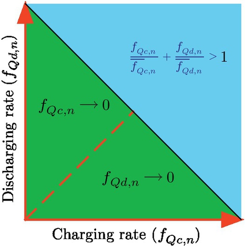
6.2 Base-case Controller
To benchmark the performance of the proposed MPC scheme, a base-case controller was developed. This base-case was meant to provide an indication of human-operator behavior during a system emergency (disturbance). Clearly, modeling a human operator is non-trivial as standard emergency procedures vary broadly across utilities. Furthermore, the experience of a human operator is not amenable to an implementable (and repeatable) algorithmic framework and, as far as the authors are aware, no data sets exist that capture operator behavior during (simulated) contingencies. However, the formulation presented here captures the underlying goals of the operator:
1. alleviate thermal overloads by rescheduling or curtailing generation, while considering ramp-rate limits and incremental generator cost curves;
2. employ sensitivity-based methods, such as power transmission distribution factors (PTDFs), generation shift factors (GSFs), and transmission loading relief (TLR) procedures to make quick control decisions to relieve thermal overloads [37];
3. shed load as an absolute last resort; and
4. ignore energy storage.
Thus, mapping the above operator traits into an MPC-based framework serves as the base case:
– Replace ΔˆTij[l]![]() with a relative overload metric:
with a relative overload metric:
ˆoij[l]=10max{0,(|fij[l]|+0.5flossij[l])/flimij−1}.
That is, if a line is 25% overloaded, ˆoij=2.5.![]()
– Consider PTDF, GSF, and TLR implicitly as onestep linear MPC process akin to Level 2 (i.e., set M = 1) and include overloads ˆoij[0|k],ˆoij[1|k]![]() in the objective and terminal costs.
in the objective and terminal costs.
– Heavily penalize load control and adjustment of SOC.
– Remove terminal constraints on overloads, Tx.![]()
– Set weighting matrices Rbase = R, Qbase = SM, and SM,base = SM.
6.3 Actual system model (plant)
The AC power flow is generally accepted as a valid representation of the actual physical power system (i.e., the plant). Therefore, the control actions recommended by the MPC, which utilizes the strictly linear model described in Section 6.1.2, is applied to an AC model of the system at each time step. This interaction between predictive DC controller and actual AC plant is illustrated in Figure 5.15. Furthermore, the resulting losses from the AC power flow are utilized in the nonlinear IEEE Standard 738 conductor temperature model to better capture the effects of MPC recommendations on the actual system. Finally, the actual energy-storage model does not allow for simultaneous charging and discharging in the same time step and instead employs the projected control action fQn[k] such that fQc,n[k]fQd,n[k] = 0.
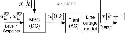
The higher the temperature, the more likely line tripping becomes. To capture the inverse relationship between temperature and expected time to trip in the actual system, the probabilistic thermal line-outage model from Section 2.1.2 is employed.
6.4 Case Study: IEEE RTS-96
The bi-level control scheme is applied to an augmented version of the IEEE RTS-96 power system test case, which is described in full details in [38]. A brief overview of this test case is included here.
6.4.1 Overview
The RTS-96 system consists of 138 kV and 230 kV subsystems. The network is organized into three interconnected physical regions, as illustrated in Figure 5.16. It consists of 73 nodes and 120 branches, of which 15 branches are in-phase transformer (IPTs), one is a phase-shifting transformer (PST), and the remainder are overhead transmission lines (138 and 230 kV). Buses are denoted with three digits: the first digit indicates the area while the latter two are intra-area designators. Bus types are indicated by color: generator (blue), load (yellow), and zero-injection (white). Edges represent transmission lines (black) and transformers (aqua/gray). The disturbance is displayed with stars: lines 113-215 and 123-217 were tripped. Note that the three underground cables in the original RTS-96 system have been replaced by equivalent overhead lines to enable application of a single thermodynamic model. Transformer temperature overloading is not considered in this case study, as their thermodynamic models differ from those presented here.

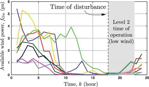
The aim of this case study is to explore the contingency management achievable with the proposed hierarchical control scheme. Unfortunately, the RTS-96 system is designed as a highly reliable system, with unusually high thermal ratings for lines. To bring the system closer to its limits and engender worthwhile scenarios, thermal ratings fijlim were reduced by 40%, yielding line temperature limits in the range of 60 to 70 °C. Furthermore, ramp rates have been reduced by 82.5% to highlight Level 2 performance and enhance the role of storage in congestion management. For the temperature dynamics, the RTS-96 system data only specifies per-unit resistance, reactance, and line length, but not the conductor types (i.e., diameter, heat capacity). Therefore, this case study employed ACSR conductors, 18/1 Waxwing (138 kV) and 26/7 Dove (230 kV), which represent reasonable choices given the reduced line ratings. The parameter values for Dove and Waxwing conductors, along with other system parameters, are provided in Table 5.7. The values in brackets represent ranges.
Table 5.7
Network model parameters used in case study
| Model Parameter | Value | Units | |
| Sampling Time, Ts | 60 | s | |
| 3-phase power base, Sb | 100 | MVA | |
| Energy-storage base, Eb | 100 | MWh | |
| Monetary unit base, Mb | 10,000 | $ | |
| Storage SOC limits, ¯Ei |
2 | pu | |
| Storage power limits, ¯fQc,¯fQd |
0.25 | pu | |
| Nominal wind power, fnomGW |
Fig. 5.17 | pu | |
| Nominal loads, fnomD |
Week 1, day 1 in [38] | pu | |
| Overcurrent protection limit, ˉΩ |
3 | - | |
| Ambient Temperature, Tamb | 35 | °C | |
| Wind speed, angle, υw ∠ θw | 0.61, π/2 | m/s, rads | |
| Line-to-line base voltage, Vb | 138 | 230 | kV |
| Thermal rating, fijlim | 1.05 | 3.00 | pu |
| Conductor diameter, Dij | 15.5 | 23.5 | mm |
| Heat capacity, mCp, ij | 383 | 916 | J/m-°C |
| Ampacity, Iijlim | 439 | 753 | A |
| Resistance per unit length, Rij | [103,118] | [55,66] | μΩ/m |
| Temperature limit, Tijlim | [62,64] | [67,71] | °C |
| Temperature coefficient, τij | 0.796 | 0.888 | - |
| Loss coefficient, ρij | 0.157 | 0.066 | °C-m/W |
| Ambient coefficient, γij | 0.193 | 0.104 | - |
| Solar heat gain rate, qs,ij | 14.4 | 21.9 | W/m |
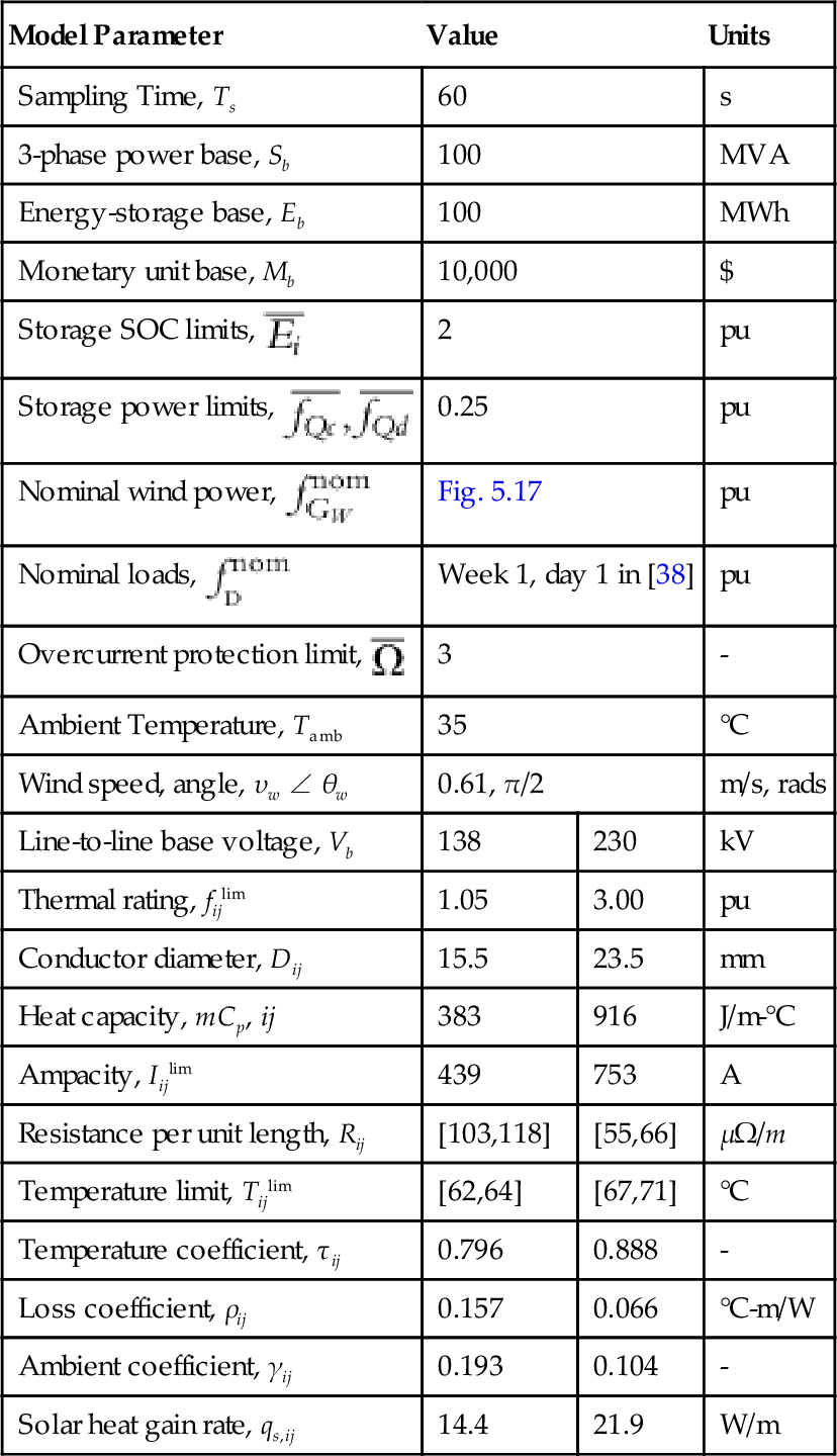
6.4.2 Optimization implementation
The objective function weighting factors utilized in MPC Level 2 and the base case are presented in Table 5.8. Note that for the base case, the overload coefficient po weights the thermal-power overload, ˆoij,![]() and not temperature. Also, the storage-control coefficient for the base case, pq = 1000, reflects the fact that this resource is not available for decision-making. Generator control actions, ΔfG, are weighted using cost-curve parameters8, with pr = max{0.05, an/maxn{an}} for Level 2, and pr = 0.1 max{0.1. an/maxn{an}} for the base case. The cost-curve parameters (an, bn) utilized in this case study are from [39, Table 1].
and not temperature. Also, the storage-control coefficient for the base case, pq = 1000, reflects the fact that this resource is not available for decision-making. Generator control actions, ΔfG, are weighted using cost-curve parameters8, with pr = max{0.05, an/maxn{an}} for Level 2, and pr = 0.1 max{0.1. an/maxn{an}} for the base case. The cost-curve parameters (an, bn) utilized in this case study are from [39, Table 1].
Table 5.8
Objective function coefficients for Q, R, and SM matrices for MPC and base case systems
| Model | po | pe | pg | pr | pw | ps | pq | pp |
| Level 2 MPC | 1 | 200 | 200 | [0.05,1] | 0.15 | 250 | 0.2 | 0.01 |
| Base Case | 1 | 0.01 | 0.01 | [0.01,0.1] | 0.5 | 500 | 1000 | 0.1 |

Recall that the early stages of a cascade evolve relatively slowly, which allows for significant computation to be performed during that period. Therefore, immediately following a disturbance, Level 1 computes new optimal set points and passes that updated information to Level 2. An overview of Level 2 operation is show in Figure 5.15.
6.4.3 Simulation results
The case study described in Section 6.4.1 is simulated in MATLAB according to Level 1, Level 2, and base-case implementations. Initially, the system is operated economically according to Level 1. However, at hour 18 (low wind, high demand), a two-line outage (i.e., the disturbance) trips lines 113-215 and 123-217. Transient (short-term) stability was assumed. Performance and behavior of the Level 2 MPC (with horizon lengths of M = 5, 10, 20, 30, and 45) and the base case are discussed below.
The double-line outage caused the remaining inter-area transmission line 107-203 to become severely overloaded (greater than 1.25fijlim). The Level 2 MPC scheme alleviated the temperature overloads and brought the system safely to the updated economic set points provided by Level 1. In contrast, the base case underwent a cascading failure, with line tripping bringing the system to a voltage collapse after 29 minutes, as exemplified by non-convergence of the AC power flow. The base-case cascading failure evolved as follows:
• k = 3: Line 107-203 tripped at ΔTij[3] = 13.5° C.
• k = 16: Line 114-116 tripped at 8.14° C.
• k = 26: Line 113-123 tripped at 11.4° C.
• k = 28: Lines 103-109 and 112-123 tripped at 16.8° C and 20.7° C.
• k = 29: Voltage collapse “blackout.”
This process is illustrated in Figure 5.18, where it can be seen that the minimum voltage magnitude fell below 0.87 pu.
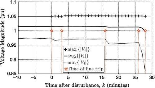
Figure 5.19a illustrates that the objective function cost (21a), calculated for each MPC run, decreased monotonically over time. This does not prove stability, but highlights the Lyapunov-like properties of the objective function [7] as MPC drives the system back to the Level 1 (economically optimal) equilibrium point.
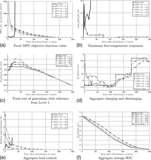
The maximum line temperatures for the base case and MPC are illustrated in Figure 5.19b. Note that MPC is able to avoid excessively high temperatures, and in fact drives all line temperatures below their respective limits by around minute k ≈ 75. Later, a few lines hover slightly above their temperature limits. However, this is due to model inaccuracy arising from MPC’s use of an approximate linear temperature model and the DC power flow. In particular, over that latter phase, the largest temperature deviations above limits are associated with 138 kV lines that exhibit X/R = 3.83 < 4. This relatively low X/R ratio engenders errors in the DC approximation of the nonlinear AC network equations. The DC model incorrectly informs the controller that losses are sufficiently low, implying that negligible control action is required for the temperature to drop below its limit in the next time step. But the actual power system, described by the AC power flow, has higher than predicted losses, and the temperature stays slightly above the limit. The controller repeats these incorrect estimates of losses until control action is required for other reasons, or load patterns autonomously reduce line loadings below limits. For k > 50, all line loadings are less than 5% above their thermal ratings, which is within expected error levels [40,41]. These results suggest that despite the presence of approximate models, the MPC scheme is able to reject the disturbance through feedback and return the system to an acceptable state. A thorough discussion of the impact of model approximations is provided in [42].
Level 2 MPC performs a balancing act between ensuring safety criteria and restoring economically optimal set points. This balance is highlighted in Figure 5.19c, where the cost of conventional generation is shown for both MPC and the base case. To ensure acceptable line temperatures, MPC initially sacrifices economic optimality by deviating from the Level 1 set points. For k > 120, the system returns to economically optimal levels, with inaccuracy in the MPC model causing some minor discrepancies. Interestingly, over the first 15 minutes or so, the generation cost achieved by MPC is actually less than the optimal cost given by Level 1. Two factors contribute to this apparent anomaly. Firstly, Figure 5.19c shows the post-disturbance Level 1 schedule, whereas the generators were initially operating according to less-costly pre-disturbance set points. Secondly, the updated Level 1 reference schedule enforces hard line-flow constraints, while MPC allows line flows to temporarily exceed limits.
As discussed in Section 6.1, the control actions available to Level 2 MPC for reducing line temperatures include: load reduction, wind curtailment, and energy-storage injections. Figure 5.19d and 5.19e illustrate the main controls employed to alleviate excessive temperatures for this case study. Contrasting MPC response with the base case, it is clear that load and energy-storage controls were crucial immediately following the disturbance. By initially curtailing energy-storage discharge (Figure 5.19d) and reducing the aggregate load by less than 5% (Figure 5.19e), line temperatures were brought to within their limits. For k ∈ [75, 240], storage discharge exceeded reference levels in order to bring SOC back to economical reference levels as displayed in Figure 5.19f. Wind curtailment was employed as cheap control over the longer term to bring and keep line temperatures below their limits.
Finally, with a shorter horizon M and the terminal constraint requiring greater use of expensive load and storage control, the MPC enjoys smaller departures in generation from the Level 1 economic reference. Such an outcome is displayed in the generation costs of Figure.5.19c. However, with a short horizon (e.g., M = 5), the controller is unable to predict the line overloads far enough in advance, which causes inferior management of energy storage and load. For example, notice in Figure.5.19f how much further away from the Level 1 reference the MPC with horizon M = 5 is compared with M ≥ 10. Considering the degree of load and storage control and line temperature profiles, a prediction horizon of M = 20 provides the best sacrifice between computational complexity and controller performance.
6.5 Data management and communication
The MPC control scheme requires a model of the network, together with measurements of the conductor temperature of (potentially) overloaded lines, SOC of energy-storage devices, output power from both conventional and renewable generation, power demand, and the operating points of all FACTS devices would be required. These data establish the initial point for the MPC prediction trajectory, and therefore must be updated every time MPC reinitializes, at the time step Ts. These measurement requirements are consistent with existing energy management system (EMS) capabilities, with topology processing establishing the network model, and state estimation providing generation and load information. Technology for measuring conductor temperature is available, though telemetry of such measurements is not currently common. It is argued in [14] and references therein, in the context of dynamic line rating, that gathering line temperatures is quite feasible. Also, a trivial modification to the MPC formulation would allow some lines to be subject to standard (hard) power-flow limits, while modeling temperature dynamics for lines that were outfitted with temperature sensors. Participation of energy-storage devices in electricity markets will likely require telemetry of their SOC. This is already the case in NYISO [43] and PJM [44].
In addition to well-defined initial conditions, MPC prediction also requires forecasts of demand, the power available from renewable generation sources, and the ambient weather conditions governing line temperatures. Generation and load forecasts are already available and used in EMS contingency analysis. Short-term weather forecasts are also typically available. Given that the MPC prediction horizon will generally be on the order of 15-30 minutes, a persistence forecast (which assumes those external influences remain unchanged) will often be adequate.
MPC broadcasts control signals at an interval of Ts ≈ 1 minute, which is much slower than other controls, such as AGC [45]. Thus, the input/output communications and data management requirements of the MPC scheme are consistent with the capabilities of existing EMS installations.
7 Summary
This chapter presents two model-predictive control (MPC) approaches to cascade mitigation in power systems. Each MPC scheme balances economic and security objectives through the use of a higher-level optimal scheduling process and a lower-level MPC strategy. The first approach represents initial efforts aimed at mitigating the effects of cascading failures in multi-energy hub systems and is based on shrinking-horizon MPC (SHMPC) with a deterministic line-outage model. The SHMPC scheme illustrates the active role of energy-storage and conversion processes and the ability of a bi-level to balance both economic and security objectives in the cascade-mitigation scheme. It is shown that energy resources must be carefully regulated because MPC has a tendency to over-exploit stored energy to the detriment of long-term energy requirements.
The ideas uncovered by the SHMPC scheme are advanced by the development of a receding-horizon MPC (MPC) cascade-mitigation scheme applied to electric-transmission systems with energy storage. The MPC design rejects disturbances (contingencies) while tracking the optimal set points established by the higher level. Disturbance rejection exploits the thermal-overload capability of transmission lines. This allows time for adjustments to be made to controllable resources that include generation levels, energy storage, and demand response. A convex relaxation is applied to the AC power flow to develop a piece-wise linear approximation for line losses. This formulation is proven to be sufficient to enable MPC to drive line temperatures below limits. As supported by an augmented IEEE RTS-96 case study, the MPC scheme can significantly improve system reliability and economic performance by leveraging the temporal nature of energy-storage and conductor temperatures.