
Electric Vehicles as Energy Storage
V2G Capacity Estimation*
K. Nandha Kumar; B. Sivaneasan; K.T. Tan; J.S. Ren; P.L. So School of Electrical and Electronic Engineering, Nanyang Technological University, Singapore
Abstract
The increase in energy consumption and the CO2 emissions of fuel-based generating sources have raised the interest in renewable energy sources (RESs). However, the inherent intermittency in the renewable power generation hinders its widespread deployment. Electric vehicles (EVs) are an important component of future transportation system and are crucial for reducing global CO2 emissions and curtailing overall energy demand. Aggregating the EVs available as smart energy storage (SES) and utilizing it for leveling the intermittent outputs of RESs is an ideal and viable prospect. The vehicle to grid (V2G) capacity, i.e., the energy/power that the EVs can supply varies over time and depends on the availability of the EVs and their individual state of charge (SOC). Hence a real-time V2G capacity estimation is important for utilizing the EVs as SES efficiently. In this chapter, a method for utilizing the EVs as SES with the aid of a real-time V2G capacity estimation algorithm is discussed.
Nomenclature
i EV number
j, l, k Half-hourly intervals
n Total number of EVs
plEV,i Predicted charging profile of an EV
pCC Contracted capacity or maximum power-demand limit
pjPD Forecasted building load demand after considering RESs
pjuEV,i Load demand of an EV
pjuEV Unscheduled total load demand of all EVs
mi Departure interval of an EV
ki Total number of intervals required for charging an EV
paverage Average power used for achieving a smooth-valley filling
pjTD Total building load demand after considering RESs and EVs
ρi Priority value of an EV
αi, βi, δi, χi Priority parameters based on battery SOC, slack time available for charging, number of intervals used for charging, and V2G power supplied, respectively
SOCi EV battery SOC in percentage
piv2g max Maximum V2G power of an EV
piv2gcont Continuous V2G power of an EV
Eiv2gav ' lable V2G energy available of an EV
SOCicurrent Current SOC of an EV
SOCifinal Desired final SOC of an EV
SOCimin Minimum required SOC for charging an EV to SOCifinal before departure time
Eiv2g max Maximum V2G energy available of an EV
piv2g V2G power available of an EV
pjact pv Actual solar PV output
pave pv Average solar PV output over a period
pjv2g required V2G power required for balancing the solar PV output
1 Introduction
The rapid urbanization with increasing population and demand for a better quality of living has led to a greater usage of energy. This has resulted in escalating pressure on the use of available resources, which are mostly fossil fuels in the form of coal, oil, and gas, leading to uncontrollable rise in air pollution. In the last few years, there has been a prolific growth in the integration of renewable energy sources (RESs) into the distribution networks in various countries [1–3]. It is expected that the penetration of RESs will increase significantly in the coming years. However, the current distribution networks are not designed to incorporate such a high penetration of RES without energy storage. The frequency and voltage fluctuations caused due to the intermittency in RES power generation have been widely reported in the United States and Europe [4].
Conversion of conventional fossil fuel-powered vehicles to electric vehicles (EVs) is considered as one of the best solutions to decreasing the emissions of the transportation sector and increasing the efficiency of the transportation system. EVs when aggregated can be treated as large smart energy storage (SES) and hence can be used to reduce the size of the energy storage required for RESs. SES can be used as a fast-responding energy source to overcome the intermittency of RESs. However, the increase in deployment of EVs will also eventually increase the load demand of the distribution network as a result of charging. Therefore, it is necessary to optimally manage the load demand, outputs of RESs, and charging/discharging of EVs to completely utilize their benefits. SES can be either used as flexible load to store power/energy when surplus power/energy is available from RESs or as a source when there is a power/energy deficit. For utilizing the SES as a source the vehicle-to-grid (V2G) capacity estimation is vital and with the help of scheduling SES can be made to behave like a flexible load. The V2G estimation methods discussed in [5] and [6] focus on using a fixed-minimum state-of-charge (SOC) limit for determining the V2G capacity, while the methods to determine the achievable power capacity for a group of EVs using plug-in probability are discussed in [7] and [8]. Hence, these methods are not suitable for real-time V2G capacity estimation and scheduling. Methods for aggregating EVs and supplying V2G power to the grid similar to [8] have also been proposed by a few authors. The aggregation process is also governed by the amount of power and energy the EVs can supply during any given interval. Using dynamic scheduling for V2G estimation as proposed in [9], the accuracy of the V2G estimation can be enhanced and also the accuracy of the estimation is not dependent on the time of estimation. A dynamic scheduling algorithm, with priority criteria, that can enhance fairness and customer satisfaction [9] is used for the V2G capacity estimation.
In this chapter, the availability of different types of RES outputs and their nature of intermittency are discussed in Section 2. The availability/travel patterns of EVs and their suitability for being used as SES for different RESs is discussed in Section 2.1. An algorithm for dynamic EV charge scheduling is discussed in Section 3. Section 4 illustrates the real-time V2G capacity estimation, which considers the main constraints on meeting the load demand while ensuring the chargeability of the EVs. In Section 5 the algorithm is applied to a typical case scenario where the EVs are used as SES for solar PV and the results are discussed.
2 Availability and Nature of Intermittency of Solar-Photovoltaic and Wind-Energy Systems
Solar photovoltaic (PV) has received increasing attention as it enables 100% renewable and zero-emission electricity production. Over the last decade, the global annual PV utilization rate has increased significantly. In 2013, it was estimated that 36.9 GW of PV systems were installed worldwide [10]. Similarly, the penetration of wind energy has also been growing rapidly in recent years and it accounts for about 1.5% of the current electricity generation around the world [11]. However, large-scale integration of RESs will put at risk the reliability and stability of the power system due to the intermittent nature of these generating sources, which can potentially result in the following problems:
a) Voltage fluctuations: When a large number of PV arrays or wind turbines are connected to the distribution network, changes in solar irradiance or wind speed will cause their output voltages to vary, which consequently results in voltage-level fluctuations at the point of common coupling (PCC). The resulting voltage fluctuations will have an adverse impact on the existing voltage-regulation schemes in the distribution network such as on-load tap-changing transformers being unable to respond to the rapid changes in the voltage levels, resulting in poor voltage regulation.
b) Frequency fluctuations: Passing clouds in the sky will result in different parts of the PV arrays being shaded, thus causing reduction in energy outputs. Similarly, lulls (sudden decrease in wind speed) in air flow caused by turbulence in the atmosphere will influence the energy outputs of wind turbines. The sudden loss of power generation from the RES will result in a drop in the power-system frequency. Furthermore, under extreme weather conditions such as thunderstorms, there could be no sunlight or wind for a certain period of time. This will result in a total loss of RES generation, leading to a drastic drop in the frequency of the distribution network.
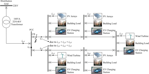
c) Increased fault level: The integration of RES into the low-voltage distribution network will lead to a more complex flow of fault currents when a fault occurs in the smart grid. These RESs, connected to the smart grid through interfacing voltage-source inverters, will alter the fault level of the low-voltage distribution network. A typical distribution system network architecture with RES integration as shown in Figure 9.1 consists of five building blocks connected in a ring topology with PV arrays and wind turbines being installed on the building rooftops. When a fault occurs on the line, which is indicated by point F as shown in Figure 9.1, there will be flow of fault currents from the RESs and the distribution grid, thus increasing the fault level at the CB connected near point F.
d) Voltage-rise problem: During the day when the sun’s irradiance is at its peak, there will be a large amount of power generated by the PV arrays. Meanwhile, at night, when the wind speed is at its peak, there will be a large amount of power generated by the wind turbines. However, the large amount of power generated might not be fully utilized (e.g., in the afternoon when the majority of the occupants are away from their houses for work or in the night when residential homes and commercial buildings use less electricity) and will result in a voltage rise at the RES outputs. This will consequently cause a voltage rise in the distribution network. The rise in voltage level might lead to tripping of the RES inverters and also equipment failures and damages.
Therefore, the active and reactive power balance in a distribution system needs to be properly controlled in order to ensure stable operation of the distribution network. Electric vehicles (EVs), which are connected to the distribution grid, can behave like energy-storage systems to compensate the RES variability, thus increasing the overall stability of the distribution network. Figures 9.2 and 9.3 show the typical daily curves of the output power from a solar PV system and a wind-energy system, respectively [1,10]. As shown in Figures 9.2 and 9.3, both PV and wind-energy systems are intermittent in their generation and have very distinct generation characteristics. It can be observed from Figure 9.2 that a solar PV system typically generates power between 7:30 am to 7:00 pm. Thus, EVs, which are usually immobile from 10:00 am to 4:00 pm, can be utilized to generate power and compensate for the variability in the power generated by the solar PV system. On the contrary, as shown in Figure 9.3, a wind-energy system has a higher power generation during the night from 7:00 pm to 6:00 am, which also corresponds to off-peak periods of energy consumption. During this period, there might be surplus of energy generated from the wind-energy system. In this case, the role of EVs is reversed and they can function as storage devices to store the surplus energy generated by the wind-energy system.


2.1 Availability and Usability of EVs
Similar to RESs, large-scale penetration of EVs that behave like flexible loads will have a significant impact on the power system and the potential to increase peak load of the power system if not managed properly [12–14]. Furthermore, if the problems are not addressed properly, it will result in decrease in power quality and increase in operation cost for the peak demand. Hence, to improve the power quality of the system, the problems should be properly addressed. The problems associated with the large-scale penetration of EVs are as follows:
a) Unpredictable increase in peak demand: The unpredictable charging of the EVs due to various mobility patterns of EV users will result in an unpredictable increase in peak demand. The uncertainty in the arrival of EVs is the main cause of this problem [14]. The various charging strategies available in the literature to mitigate this problem focus mainly on personal vehicles parked at individual houses and small buildings [12–17]. Such strategies are not suitable for urban cities where 70 to 80% of the buildings are high-rise multi-story buildings.
b) Voltage fluctuations and increased total harmonic distortion: EV charging involves the conversion of power through power electronic devices, which will result in increased voltage fluctuations, harmonic distortions, and power losses. The problems will be more serious if charging happens during peak demand [15]. All the methods available in the literature primarily focus on shifting the charging demand from peak period to off-peak period in order to reduce the problems related with EV charging. However, such an approach will not ensure an optimal solution to these problems. The increased power losses and total harmonic distortion (THD) problems associated with different battery-charging modes must also be considered.
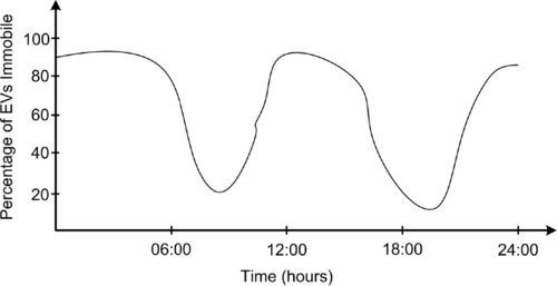
However, if EV charging/discharging is managed properly, it is not only possible to mitigate these problems but also possible to derive many auxiliary functions such as distributed reserves for renewable energy [18–20]. For utilizing the EVs as SES, the availability of the EVs should be considered. The availability of EVs can be obtained from the traveling patterns of different types of EVs. EVs have traveling ranges usually between 90 to 160km, which is well within the average travel distance in urban cities. The availability of EVs has an inherent variability, but it can be predicted to a certain level of accuracy, which makes EVs highly suitable for being utilized as SES. Based on research conducted by the authors in [12,21], and [22], it was found that most EVs are immobile 90% of the day. The time during which the EVs are immobile and available to be used as SES is shown in Figure 9.4. It can be observed that the majority of the EVs are generally used for transportation to and from work between the hours of 8:00 am and 10:00 am and from 4:00 pm to 8:00 pm, respectively. These are the time periods when the EV availability as SES is low. However, during peak hours (i.e., between 10:00 am and 2:00 pm) and off-peak hours (i.e., between 10:00 pm and 5:00 am) the EVs are usually not used or immobile as they are typically plugged in for charging at the workplace and home car park, respectively. These are the time periods when the EV availability as SES is high. Hence, during off-peak hours, the EVs can be used as flexible load to store the additional energy generated by RESs, particularly wind turbines, and can be used as a source during peak hours to accomodate for the intermittency of RESs, particularly solar.
3 EV Charge-Scheduling Algorithm
Coordinated charging of EVs is the most effective method for integrating a large number of EVs into an existing power system. In this method, the charging of EVs is controlled such that optimal performance can be obtained while power-system stability and reliability is not jeopardized. There are various coordinated charging strategies available in the literature, which can be classified into two broad groups: power-controlled [12,23] and time-controlled [24–27] coordinated charging. EV charge scheduling is an important component in both power-controlled and time-controlled coordinated charging methods. Though there are various scheduling algorithms available in the literature, dynamic scheduling is inevitable in order to account for the unpredictable load demand. The dynamic scheduling algorithms such as least laxity first (LLF) and earliest deadline first (EDF) are widely used for EV charge scheduling [28–30].
The dynamic scheduling algorithm discussed in this chapter uses a data-driven scheduling approach to overcome the disadvantages of existing scheduling methods, while providing a more robustness algorithm compared to those available in the literature. The load models used are forecasted load demand without EVs [31] and predicted EV charging profiles [32]. In the proposed algorithm various dynamic priority criteria are used for scheduling the EV charging. The priority criteria are chosen such that customer satisfaction and fairness are maximized. The dynamic priority criteria considered by the scheduling algorithm are based on i) SOC of EV battery, ii) slack time available for charging, iii) time/energy already allotted for the EV, and iv) V2G power already supplied. The objective function of the scheduling algorithm is to minimize the variance in priority values of the connected EVs during all the intervals throughout the charging period. Minimizing the variance in priority values of the EVs will reduce the variations in fairness given to the EVs and also increase customer satisfaction.
The algorithm utilizes day-ahead half-hourly forecasted load demand without EVs pjL, predicted EV charging profile plEV,i, predicted output of RESs pjRES, power-demand constraint pCC, and number of allotted charging intervals njEV,i for each EV. Half-hour intervals in a day are represented by subscript j = 1, 2, 3… 48. If k is the total number of charging intervals required for charging a particular EV, then subscript l = 1, 2, 3… k. EV ID is given by the superscript i, and it takes the values 1, 2, 3… n, where n is the total number of EVs. The charge schedule is updated every half hour considering 30-minute electricity-price intervals. The forecasted load demand taking RES outputs into consideration is given by:
The unscheduled total demand of EVs is given by:

where mi is the departure interval of ith EV, ki is the total number of intervals required for charging the ith EV, and l is given by:
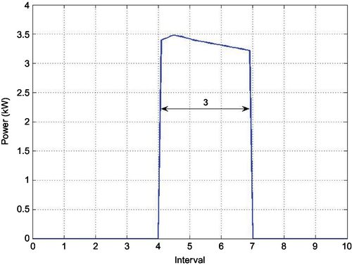
In order to clearly illustrate the unscheduled total demand of EVs as given by (2), a typical example with mi = 8 and ki = 3 is shown in Figure 9.5, where each interval corresponds to 30 minutes. Based on (3), l is less than or equal to zero up to j = 3 and greater than 3 for j > 7. This means that plEV,i is “0” for the 2 intervals (i.e., intervals 2 and 3) and when l becomes “1” at j = 4 and “4” at j = 7, then plEV,i will have a positive value. Hence, based on (2), pjuEV,i is “0” for 1 ≤ j < 4 and j ≥ 8, and pjuEV,i is equal to plEV,i for 4 ≤ j ≤ 7. Similarly, this method can be used to obtain the load demand of each EV.
The maximum value of mi gives the interval in which the last EV departs and is represented as:
The departure interval-selection process is denoted by σ and the propositional formula to select the departure interval of the last EV to depart is denoted by the subscript “max.” Smooth-valley filling is required for optimal power-system operation [25], and the average power required for having a smooth-valley filling is obtained by:

where

The algorithm considers the contracted capacity or maximum power-demand limit pCC and the average power used for achieving a smooth-valley filling paverage for obtaining the EV charging schedule (CS) matrix in the form:
where  and xi,j is the control signal broadcasted to the EV charging station to charge or discharge the battery. The control signal for each EV connected to a charging station is represented by a corresponding row in the CS matrix for the next 48 half-hour intervals. The values of xi,j are obtained by subjecting the total load demand after considering RESs and EVs pjTD to the following conditions:
• the additional load due to EV charging does not exceed x% of pCC; and
• pjTD does not exceed paverageby y% of paverage.
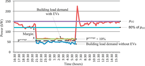
The first constraint is to ensure that the EVs scheduled for charging will not exceed the maximum power-demand limit and thus overload the power system. The second constraint is required to achieve a smooth-valley filling and higher energy efficiency [25]. Therefore, each half-hour interval in the EV charge scheduling (i.e., a total of 48 intervals) will have an optimum number of EV charging. Furthermore, 24-hour scheduling helps to spread the EV load without violating owner’s satisfaction and comfort. The value of x should be selected such that the total demand of the building is always within the maximum power-demand limit. The actual value of x can be determined based on either an heuristic approach or statistical data on load demand. The choice of x is determined based on the ability of the demand-response algorithm used by building energy-management system (BEMS) to curtail the total load demand below pCC. For example, in a building 80% of pCC can be used as the limit for controlling the EV demand, while 85% of pCC can be used as the limit for controlling HVAC demand and 90% of pCC can be used as the limit for shedding other interruptible loads. Hence, if the EVs are scheduled for charging when the total demand is greater than 80% of pCC, the charging will be interrupted by the demand-response algorithm. The second condition is that pjTD cannot be greater than y% of paverage to ensure that the EVs are charged to the desired SOC and a smooth-valley filling is achieved. A typical example, as shown in Figure 9.6, is used to explain the above condition. If 10% of paverage is considered as the additional limit for scheduling the EV charging, all the EVs can be charged to the desired SOC and a smooth-valley filling is achieved during the off-peak period. Furthermore, the margin to exceed the 80% of contracted capacity is sufficiently large so that EV charging will not be interrupted. We take 10% of paverage to accommodate for charging more EVs without exceeding 80% of the contracted capacity during the off-peak period.
The sequence in which an EV is added to pjTD depends on the priority value of EVs. In the algorithm, various dynamic priority criteria are used for scheduling the EV charging. The priority criteria are chosen such that customer satisfaction and fairness are maximized. The dynamic priority criteria considered by the scheduling algorithm are based on:
• Battery SOC: αi represents the priority parameter due to battery SOC. The customer’s satisfaction will be higher if the EV can be charged to the desired SOC before departure. As expressed in (9), the priority value will decrease with increase of SOC, so the EV with a lower SOC will have a higher priority value. This parameter is essential for achieving higher customer satisfaction. SOCi is the particular EV’s battery SOC in percentage.
• Slack time available: βi represents the priority parameter due to the slack time available for charging. Slack time is the difference between the time available before departure and time required to complete charging, e.g., an EV arrives at 12:00 pm and will depart at 6:00 pm. If 3 hours is the time required to complete charging, then the slack time is 3 hours. With higher slack time, the feasibility of charging the EV to desired SOC is higher. The priority value will decrease with increase in slack time, which will enable the EV with lower slack time to have higher priority for charging as expressed in (10). This parameter is required to ensure higher degree of fairness to the EV owners. Ndep,i is the number of half-hour time intervals from current time to departure time for the particular EV. Nreq,i is the number of half-hour time intervals required for charging the particular EV up to the required SOC.
• Number of intervals used for charging: δi represents priority parameter due to completed charging intervals. The number of intervals used for charging the EV represents amount of resources already allocated, hence the higher the number of intervals used, the lower will be the priority for charging as indicated in (11). This parameter is also required to ensure higher degree of fairness to the EV owners. Ncom,i is the equivalent number of half-hour time intervals completed for charging the particular EV.
• V2G power supplied: χi represents the priority parameter due to V2G power/energy supplied by the EV. The higher the number of intervals in which the EV supplied V2G power, the higher will be the priority for charging the EV as shown in (12). This parameter is essential for achieving higher customer satisfaction. Nv2g,i is the equivalent number of half-hour time intervals during which the EV is supplying power. Ntotal,i is the equivalent number of half-hour time intervals required for charging the EV from initial to desired SOC.
The EV priority value is then given by:
where


w1, w2, w3, and w4 are the weighing factors for the priority parameters due to battery SOC, slack time, completed charging intervals, and V2G power supplied, respectively. i is the EV number. It is evident from (8) that the values of w1, w2, w3, and w4 can be tuned to overcome the unequal preference given by each priority criterion toward a particular type of EV and ensure equal degree of fairness to all the EVs. These values can be determined through stochastic or data-driven simulations in order to ensure a higher degree of fairness and customer satisfaction. These values can also depend on the policies used for charging and discharging the EVs. For example, if the operator wishes to give a higher priority (say 25% higher) to an EV with very low SOC, then the value of w1 can be selected as 2 instead of 1. This will result in an increase in the priority value by 25%. Since there are four priority parameters, each weighing factor accounts for 25% of the priority value, thus increasing the value of any one of the weighing factors by 1 will increase the priority value by 25%. As another example, if the operator wishes to give a higher priority (say 50% higher) to an EV that supplies V2G power during peak hours, then the value of w4 can be selected as 3 instead of 1. This will result in an increase in the priority value by 50%. The values of the weighing factors can also be determined through stochastic simulations in order to ensure a higher degree of fairness and customer satisfaction.
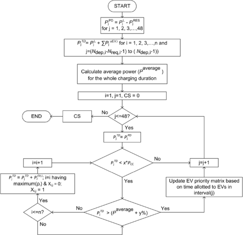
The flow chart of the EV charge-scheduling algorithm presented in [9] is shown in Figure 9.7. In the first step, the load demand without EVs is obtained using (1). In the second step, the load demand due to the addition of EV load is obtained from (2), (3), and (6). This is then superimposed on the load demand without EVs obtained from (1) and the total load demand with EVs is obtained. The average load demand is calculated for a whole charging period using (4) and (5) as the next step. The initialization of the EV charging-schedule matrix to a zero matrix is carried out in fourth step. The modification of the EV charging-schedule matrix values, which determine the EVs allowed to be charged during each interval, is executed in the fifth step. This step is repeated for all 48 intervals. The priority value of each EV, the power limits (if any), and the average power during the charging period determines the number of EVs that are allowed to be charged in a given interval. The priority values not only change dynamically during every half-hour interval based on the current status of the EVs but also during the scheduling process based on the expected status of the EVs. The EV charge-scheduling algorithm along with real-time demand response ensures that the power limits are never violated and the outputs of RESs are optimally used so that the operation cost can be minimized.
4 V2G Capacity-estimation Method
V2G is a concept in which energy from EV is supplied to the grid. Various other terminologies such as vehicle to home (V2H) and vehicle to building (V2B) are also commonly used. V2G can be used for many applications such as to supply additional energy during periods of maximum demand or high electricity price. However, as V2G requires using a fraction of battery life, EV users may be reluctant to enter into an agreement with building operators unless there are considerable monetary or convenience benefits.
The V2G concept also enables the utilization of EV batteries as storage for leveling the intermittency of RESs. For utilizing EV batteries as SES, V2G capacity has to be estimated in real-time for efficient and optimum control of the V2G operation. The V2G estimation methods available in the literature mainly focus on determining the achievable power capacity for a group of EVs [5,17]. Apart from the capacity estimation, other methods have been proposed for aggregating EVs and supplying V2G power to the grid [8,33]. The aggregation process is also governed by the amount of power and energy that the EVs can supply during any given interval. The V2G capacity estimation can be based on many factors/constraints, but the two most important factors to be considered in V2G capacity estimation are discussed below [9].
4.1 Maximum and Continuous V2G Power
The ratings of the power electronic converters used for charging and discharging the EV batteries impose the limits on the maximum V2G power piv2g max and continuous V2G power piv2gcont. Generally, the power ratings of EV batteries are considerably higher than the ratings of their power electronic converters. This implies that piv2g max and piv2gcont are not constrained by the battery-power ratings, e.g., the continuous power of Mitsubishi’s MiEV battery is 80 kW and the continuous power of its power electronic converter is 2.5 kW [34]. piv2g max and piv2gcont are basic necessities for determining the cumulative power that a group of EVs can supply during a given interval.
4.2 V2G Energy Available
The ability of the system to charge the EV to its required SOC at departure so as to satisfy the travel needs of the owner is crucial. Hence, the chargeability and drivability of the EVs is to be ensured before utilizing the EVs for auxiliary functions such as V2G. The V2G energy available Eiv2gav ' lable from each EV depends on the current state of charge SOCicurrent, desired final state of charge SOCifinal, and minimum required state of charge SOCimin at the end of current interval for charging the EV to SOCifinal before departure time.
The flow chart of the V2G capacity-estimation algorithm is shown in Figure 9.8. The chargeability and drivability of the EVs can only be ensured by the EV charge-scheduling algorithm, and hence the scheduling algorithm forms the basic block for V2G capacity estimation. The V2G capacity estimation is carried out at the beginning of every half-hour interval. It can be seen from Figure 9.8 that the V2G capacity estimation has two processes, one every 30 minutes and the other one every minute. The first process, which is executed every 30 minutes, calculates the minimum SOC required for each EV at the end of the current interval so that the EVs can be charged completely before departure. The scheduling algorithm shown in Figure 9.7 is used to determine the chargeability of the EVs considering the calculated minimum required SOC as the current SOC of the next interval. If the estimated SOC at the last departure interval is less than the desired SOC, the minimum required SOC is then increased by r% (say 5%) and the whole process is repeated. All the above four steps are shown under the condition “Time = xx: 30 or xx: 60” in Figure 9.8. Meanwhile, the second process, which is executed every minute, tracks the amount of energy supplied during the current interval and updates the results as shown under the condition “Time = xx: xx: 59” in Figure 9.8.

The maximum energy that can be supplied by each EV during a given interval is:
The time factor τ has a value of 0.5 as a 30-minute interval is considered and changes accordingly with the changes in the time period of the interval. The SOCimin is calculated to start the estimation process. SOCimin is the minimum required SOC at the end of current half-hour interval for achieving the SOCifinal of each EV before their respective departure interval. SOCimin is initialized such that the maximum energy can be supplied during the given interval and the chargeability of EV is verified using EV scheduling. If the chargeability is violated, then SOCimin is iteratively increased and verified using EV scheduling until the chargeability is not violated. Equations (14) and (15) are then used to calculate the V2G energy the EV can supply in the current half-hour interval.
where Ci is the energy capacity of the ith EV.

Eiv2gav ' lable in (15) is restricted to Eiv2g max, which is the limitation imposed by the power electronic converters used for charging and discharging the EV batteries. Using the V2G energy available, the V2G power available can be determined by:

where τ1 is the actual time for which the V2G power is supplied or can be supplied during the given interval. piv2g will vary depending on the value of τ1. However, it is limited to piv2g max and is governed by the short time rating of the power electronic converter and the battery. Therefore, the continuous power that can be provided through V2G is given by:
The estimated V2G capacity for the current half-hour interval updates every minute in order to account for the actual energy and power supplied during the particular interval. The total V2G energy and V2G power available from a group of EVs is given by (18) and (19), respectively.


The feedback on charging status is received only once after each 30-minute interval, and the V2G estimation using dynamic scheduling is executed only at xx:30 or xx:00 (e.g., 1:30 or 2:00), which avoids any positive feedback on the estimation during the charging. Subsequently, every minute estimation at xx:xx:59 (e.g., 13:30:59) within a particular interval is performed to determine only the real-time V2G power without re-estimation using EV scheduling. The re-estimation using EV scheduling will only occur at the end of the interval. Hence, the stability issues related to positive feedback to the EV charging are avoided.
5 Case Study
The algorithm is applied to case-study scenario using BEMS employed in an office building. It is assumed that the building is equipped with 70 kWp solar PV installed on its rooftop. The maximum power Piv2gcont for an EV is fixed at 3.4 kW, corresponding to a level II charger of Nissan Leaf. In an EV fleet connected to an office building the number of EVs available during office hours (8:30 am to 5:30 pm) is significantly higher than the number of EVs available in non-office hours (5:30 pm to 8:30 am). So the EVs are used as SES for the solar PV from 8:30 am to 5:30 pm. Hence, the V2G capacity of EVs parked at the office building is significantly large during office hours and offers feasibility for using EV batteries as SES for an intermittent solar PV system installed in the office building. The predicted output of a solar PV system rated at 70 kWp during office hours from 8:30 am to 5:30 pm is shown in Figure 9.9. The predicted solar PV output is obtained using the irradiance data of a typical day in Singapore. The average solar PV output pave pv for the period of operation can be determined using the method explained in [35].

The amount of V2G power required to accomodate the intermittency of solar PV is based on the difference between the actual solar PV output power and average solar PV output power as given by:
where pjact pv and pjv2g required are the actual solar PV output and V2G power required during the intervals j = 1, 2, 3…48. When pjv2g required is negative, the V2G power available from the EVs will be used to balance the power shortage and when pjv2g required is positive, surplus solar PV output power will be used to charge the EV. It is assumed that no EV is allowed to discharge (V2G) below 50% of the SOC to ensure that the minimum required SOC at departure can be achieved for all the EVs. However, the possibility that the available V2G power is less than the power deficit of solar PV is nearly remote. To clearly show the difference between using EVs as SES for solar PV and using EVs as SES along with solar PV for peak shaving, similar system parameters used in case study B of [9] where an office building with a contracted capacity pCC of 270 kW and a typical EV fleet as shown in Table 9.1 are considered.
Table 9.1
Typical EV Fleet of an Office Building
| EV ID (i) | Capacity (kWh) | Initial SOC (%) | Minimum Desired SOC (%) | Arrival Time (hr) | Departure Time (hr) |
| 1 | 24 | 83.96 | 83.96 | 08:12 | 17:30 |
| 2 | 24 | 72.08 | 72.08 | 08:34 | 17:16 |
| 3 | 24 | 80.48 | 80.48 | 07:59 | 17:40 |
| 4 | 24 | 65.52 | 65.52 | 07:58 | 17:13 |
| 5 | 24 | 68.00 | 68.00 | 08:02 | 17:59 |
| 6 | 24 | 61.23 | 61.23 | 09:01 | 17:14 |
| 7 | 24 | 70.52 | 70.52 | 08:39 | 17:48 |
| 8 | 24 | 75.52 | 75.52 | 08:37 | 17:14 |
| 9 | 24 | 69.10 | 69.10 | 08:14 | 17:50 |
| 10 | 24 | 69.10 | 69.10 | 07:58 | 18:13 |
| 11 | 24 | 75.17 | 75.17 | 08:10 | 17:05 |
| 12 | 24 | 64.10 | 64.10 | 08:28 | 17:34 |
| 13 | 24 | 72.33 | 72.33 | 08:07 | 17:18 |
| 14 | 24 | 70.56 | 70.56 | 08:43 | 18:08 |
| 15 | 24 | 63.48 | 63.48 | 07:58 | 17:51 |

Table 9.1 is obtained by considering the average travel distance of 55 km for Singapore’s personal vehicles [36], and it is assumed that the distance traveled by personal vehicles follows a normal distribution with a standard deviation of 10 km [36]. The arrival time and departure time of the EVs are assumed to be normally distributed between 8:30 am and 5:30 pm, respectively, with a standard deviation of 30 minutes. In an EV fleet connected to an office building, the EVs would have completed only one-way travel, which is approximately half the average per day travel distance. This is depicted in Table 9.1, according to which the average initial SOC is 70.74%. The EV users will be reluctant to allow the building operators to use their EVs as SES if the SOC at the time of departure is lower than the initial SOC. This is due to range anxiety which is defined as fear of running out of charge during a journey. Hence, the initial SOC and the desired SOC at the departure are considered to have same values. However, the maximum SOC to which the EVs can charge is set to 100% so as to enable complete utilization of the solar PV power, and EVs can be charged beyond the minimum desired SOC at departure during power surplus, which can be later utilized during a power shortage.
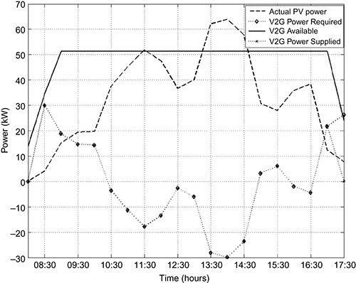
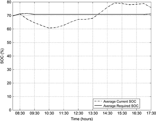
pjact pv, pjv2g required, and pjv2gtotal between 8:30 am and 5:30 pm are shown in Figure 9.10, while the average current SOC and the minimum required SOC of all the EVs are shown in Figure 9.11. From Figure 9.10, it can be inferred that during the morning hours, i.e., from 8:30 am to 10:30 am, pjact pv is less than the estimated pave pv due to comparatively less solar irradiation. Hence, the EV batteries are used to supplement the power deficit in comparison to pave pv. It can also be observed that pjv2g required is well within the limits of pjv2gtotal as the EVs are generally charged to the maximum possible SOC using the cheaper power available during the off-peak hours, i.e., from 7:00 pm to 6:00 am, and also as the EVs have traveled only half of their daily traveling distance. For example, the pjv2g required from 10:00 am to 10:30 am is 14.29 kW but pjv2gtotal during the same interval is significantly higher at 51.41 kW. This is mainly due to the fact that the possibility of charging the EVs to the desired SOC is very high as sufficient time is available for charging the EVs before departure. From Figure 9.11, the decrease in average SOC during the time period of 8:30 am to 10:30 am illustrates the discharging of EV batteries during this time interval, while from 10:30 am to 3:00 pm due to strong solar irradiation, pjact pv is greater than the estimated pave pv and hence the EV batteries are used to store the surplus power generated by solar PV. This subsequently increases the average SOC during the time period between 10:30 am and 3:00 pm as shown in Figure 9.11. However, when pjact pv becomes less than pave pv from 3:00 pm to 4:00 pm possibly due to some cloud covering, the EV batteries, which were sufficiently charged during the period from 10:30 am to 3:00 pm, yields a pjv2gtotal of 51.41 kW, which is much higher compared to the pjv2g required of 3.27 kW from 3:00 pm to 3:30 pm and 6.05 kW from 3:30 pm to 4:00 pm, respectively. The operation of the EV batteries during the period from 4:00 pm to 5:00 pm is similar to the charging operation from 10:30 am to 3:00 pm, while the operation of the EV batteries during the period from 5:00 pm to 5:30 pm is similar to the discharging operation from 3:00 pm to 4:00 pm. Comparing Figures 9.10 and 9.11 to the Figures 6(a) and 6(b) of [9], it can be clearly seen that the depth of discharge of EV batteries when used as SES for solar PV is less compared to the depth of discharge when used as SES for peak shaving. Since the battery life is inversely proportional to the depth of discharge, using EV batteries as SES for solar PV is beneficial in terms of prolonging the EV battery life cycle compared to using it for peak shaving. Furthermore, the V2G capacity is also higher and much more stable when EV batteries are used as SES for solar PV.
Using the same system parameters as in the previous case study, if a sudden loss of solar PV power for a particular time period is implicated, then the importance of using scheduling for V2G capacity-estimation can be realized. For example, let us assume that PV power is lost between 1:00 pm and 3:00 pm due to sudden weather condition such as heavy rain as highlighted in Figure 9.12. The changes in pjv2gtotal, which can be observed from Figure 9.12, show that pjv2gtotal drops drastically after supplying pave pv of 34.03 kW, i.e., the estimated average power from solar PV for three continuous intervals between 1:00 pm and 2:30 pm. From 2:30 pm to 3:00 pm, although the required V2G power is 34.03 kW, only 6.8 kW is available from the EVs. This is due to the fact that the average current SOC has reduced to 52.89%, as shown in Figure 9.13, which means that in order to ensure chargeability of the EVs before departure, no more than 6.8 kW can be supplied as V2G power. Without a charge-scheduling algorithm, if 34.03 kW instead of 6.8 kW was also supplied for the period from 2:30 pm to 3:00 pm, the EVs would not be able to charge up to the desired SOC before departure and thus cause inconvenience and dissatisfaction to EV owners.


Table 9.2 compares the accuracy of V2G capacity estimation using dynamic scheduling with two other methods using fixed minimum SOC limited estimation [8,9] and plug-in probability based estimation [10,11]. The comparison is carried out to illustrate the impact of discharging in subsequent intervals, which is a common phenomenon when the PV power is lost due to unexpected weather conditions. The comparison is performed using stochastic load demand and stochastic EV demand. Three scenarios, namely, scenarios 1, 2, and 3, where EVs are discharged to supply V2G power from 10:00 am to 10:30 am, 1:00 pm to 1:30 pm, and 4:00 pm to 4:30 pm, respectively, are considered for the comparison. It can be observed from Table 9.2 that the estimation accuracy of the methods, which do not employ scheduling of EVs, decreases with an increasing number of subsequent discharging intervals. It can be seen that in scenario 3, the average deviation of actual final SOC from desired final SOC when the EVs are not charged is higher at 3.74% and 3.05% for the fixed-minimum SOC limited estimation and plug-in probability based estimation methods, respectively, compared to only 0.92% for the V2G capacity estimation using dynamic scheduling. This indicates that the accuracy of V2G capacity estimation using dynamic scheduling is not affected by the number of subsequent discharging intervals or the time of estimation.
Table 9.2
Comparison of V2G Estimation Accuracy
| Scenario | Dynamic Scheduling | Fixed SOC Limited | Plug-in Probability | |||
| P1 | P2 (%) | P1 | P2 (%) | P1 | P2 (%) | |
| 1 | 0.9848 | -0.65 | 0.9223 | -0.98 | 0.9189 | -0.95 |
| 2 | 0.9852 | -0.83 | 0.9266 | -0.93 | 0.9011 | -0.97 |
| 3 | 0.9803 | -0.92 | 0.9147 | -3.74 | 0.9095 | -3.05 |
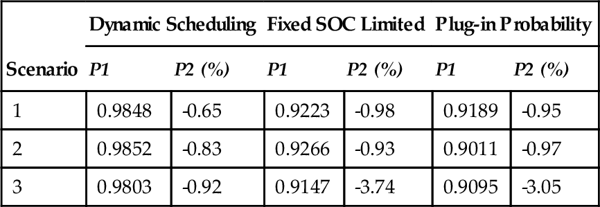
Note:
P1 - Probability of charging the EVs to the desired SOC if the required V2G power is supplied in any given interval
P2 - The average deviation of actual final SOC from desired final SOC when the EVs are not charged to the desired SOC