
Chapter 13
Parallel Programming and Computational Thinking
Chapter Outline
13.1 Goals of Parallel Computing
13.2 Problem Decomposition
13.3 Algorithm Selection
13.4 Computational Thinking
13.5 Summary
13.6 Exercises
We have so far concentrated on the practical experience of parallel programming, which consists of CUDA programming model features, performance and numerical considerations, parallel patterns, and application case studies. We will now switch gear to more abstract concepts. We will first generalize parallel programming into a computational thinking process of decomposing a domain problem into well-defined, coordinated work units that can each be realized with efficient numerical methods and well-known algorithms. A programmer with strong computational thinking skills not only analyzes but also transforms the structure of a domain problem: which parts are inherently serial, which parts are amenable to high-performance parallel execution, and the trade-offs involved in moving parts from the former category to the latter. With good problem decomposition, the programmer can select and implement algorithms that achieve an appropriate compromise between parallelism, computational efficiency, and memory bandwidth consumption. A strong combination of domain knowledge and computational thinking skills is often needed for creating successful computational solutions to challenging domain problems. This chapter will give readers more insight into parallel programming and computational thinking in general.
13.1 Goals of Parallel Computing
Before we discuss the fundamental concepts of parallel programming, it is important for us to first review the three main reasons why people adopt parallel computing. The first goal is to solve a given problem in less time. For example, an investment firm may need to run a financial portfolio scenario risk analysis package on all its portfolios during after-trading hours. Such an analysis may require 200 hours on a sequential computer. However, the portfolio management process may require that analysis be completed in four hours to be in time for major decisions based on that information. Using parallel computing may speed up the analysis and allow it to complete within the required time window.
The second goal of using parallel computing is to solve bigger problems within a given amount of time. In our financial portfolio analysis example, the investment firm may be able to run the portfolio scenario risk analysis on its current portfolio within a given time window using sequential computing. However, the firm is planning on expanding the number of holdings in its portfolio. The enlarged problem size would cause the running time of analysis under sequential computation to exceed the time window. Parallel computing that reduces the running time of the bigger problem size can help accommodate the planned expansion to the portfolio.
The third goal of using parallel computing is to achieve better solutions for a given problem and a given amount of time. The investment firm may have been using an approximate model in its portfolio scenario risk analysis. Using a more accurate model may increase the computational complexity and increase the running time on a sequential computer beyond the allowed window. For example, a more accurate model may require consideration of interactions between more types of risk factors using a more numerically complex formula. Parallel computing that reduces the running time of the more accurate model may complete the analysis within the allowed time window.
In practice, parallel computing may be driven by a combination of the aforementioned three goals. It should be clear from our discussion that parallel computing is primarily motivated by increased speed. The first goal is achieved by increased speed in running the existing model on the current problem size. The second goal is achieved by increased speed in running the existing model on a larger problem size. The third goal is achieved by increased speed in running a more complex model on the current problem size. Obviously, the increased speed through parallel computing can be used to achieve a combination of these goals. For example, parallel computing can reduce the runtime of a more complex model on a larger problem size.
It should also be clear from our discussion that applications that are good candidates for parallel computing typically involve large problem sizes and high modeling complexity. That is, these applications process a large amount of data, perform many iterations on the data, or both. For such a problem to be solved with parallel computing, the problem must be formulated in such a way that it can be decomposed into subproblems that can be safely solved at the same time. Under such formulation and decomposition, the programmer writes code and organizes data to solve these subproblems concurrently.
In Chapters 11 and 12 we presented two problems that are good candidates for parallel computing. The MRI reconstruction problem involves a large amount of k-space sample data. Each k-space sample data is also used many times for calculating its contributions to the reconstructed voxel data. For a reasonably high-resolution reconstruction, each sample data is used a very large number of times. We showed that a good decomposition of the FHD problem in MRI reconstruction is to form subproblems that each calculate the value of an FHD element. All these subproblems can be solved in parallel with each other. We use a massive number of CUDA threads to solve these subproblems.
Figure 12.11 further shows that the electrostatic potential calculation problem should be solved with a massively parallel CUDA device only if there are 400 or more atoms. A realistic molecular dynamic system model typically involves at least hundreds of thousands of atoms and millions of energy grid points. The electrostatic charge information of each atom is used many times in calculating its contributions to the energy grid points. We showed that a good decomposition of the electrostatic potential calculation problem is to form subproblems that each calculate the energy value of a grid point. All the subproblems can be solved in parallel with each other. We use a massive number of CUDA threads to solve these subproblems.
The process of parallel programming can typically be divided into four steps: problem decomposition, algorithm selection, implementation in a language, and performance tuning. The last two steps were the focus of previous chapters. In the next two sections, we will discuss the first two steps with more generality as well as depth.
13.2 Problem Decomposition
Finding parallelism in large computational problems is often conceptually simple but can be challenging in practice. The key is to identify the work to be performed by each unit of parallel execution, which is a thread in CUDA, so that the inherent parallelism of the problem is well utilized. For example, in the electrostatic potential map calculation problem, it is clear that all atoms can be processed in parallel and all energy grid points can be calculated in parallel. However, one must take care when decomposing the calculation work into units of parallel execution, which will be referred to as threading arrangement. As we discussed in Section 12.2, the decomposition of the electrostatic potential map calculation problem can be atom-centric or grid-centric. In an atom-centric threading arrangement, each thread is responsible for calculating the effect of one atom on all grid points. In contrast, a grid-centric threading arrangement uses each thread to calculate the effect of all atoms on a grid point.
While both threading arrangements lead to similar levels of parallel execution and same execution results, they can exhibit very different performance in a given hardware system. The grid-centric arrangement has a memory access behavior called gather, where each thread gathers or collects the effect of input atoms into a grid point. Figure 13.1(a) illustrates the gather access behavior. Gather is a desirable thread arrangement in CUDA devices because the threads can accumulate their results in their private registers. Also, multiple threads share input atom values, and can effectively use constant memory caching or shared memory to conserve global memory bandwidth.
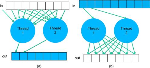
Figure 13.1 (a) Gather and (b) scatter based thread arrangements.
The atom-centric arrangement, on the other hand, exhibits a memory access behavior called scatter, where each thread scatters or distributes the effect of an atom into grid points. The scatter behavior is illustrated in Figure 13.1(b). This is an undesirable arrangement in CUDA devices because the multiple threads can write into the same grid point at the same time. The grid points must be stored in a memory that can be written by all the threads involved. Atomic operations must be used to prevent race conditions and loss of value during simultaneous writes to a grid point by multiple threads. These atomic operations are much slower than the register accesses used in the atom-centric arrangement. Understanding the behavior of the threading arrangement and the limitations of hardware allows a parallel programmer to steer toward the more desired gather-based arrangement.
A real application often consists of multiple modules that work together. The electrostatic potential map calculation is one such module in molecular dynamics applications. Figure 13.2 shows an overview of major modules of a molecular dynamics application. For each atom in the system, the application needs to calculate the various forms of forces (e.g. vibrational, rotational, and nonbonded) that are exerted on the atom. Each form of force is calculated by a different method. At the high level, a programmer needs to decide how the work is organized. Note that the amount of work can vary dramatically between these modules. The nonbonded force calculation typically involves interactions among many atoms and incurs much more calculations than the vibrational and rotational forces. Therefore, these modules tend to be realized as separate passes over the force data structure. The programmer needs to decide if each pass is worth implementing in a CUDA device. For example, he or she may decide that the vibrational and rotational force calculations do not involve a sufficient amount of work to warrant execution on a device. Such a decision would lead to a CUDA program that launches a kernel that calculates nonbonding forces for all the grid points while continuing to calculate the vibrational and rotational forces for the grid points on the host. The module that updates atomic positions and velocities may also run on the host. It first combines the vibrational and rotational forces from the host and the nonbonding forces from the device. It then uses the combined forces to calculate the new atomic positions and velocities.
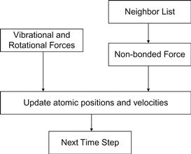
Figure 13.2 Major tasks of a molecular dynamics application.
The portion of work done by the device will ultimately decide the application-level speedup achieved by parallelization. For example, assume that the nonbonding force calculation accounts for 95% of the original sequential execution time and it is accelerated by 100× using a CUDA device. Further assume that the rest of the application remains on the host and receives no speedup. The application-level speedup is 1/(5%+95%/100)=1/(5%+0.95%)=1/(5.95%)=17×. This is a demonstration of Amdahl’s law: the application speedup due to parallel computing is limited by the sequential portion of the application. In this case, even though the sequential portion of the application is quite small (5%), it limits the application-level speedup to 17× even though the nonbonding force calculation has a speedup of 100×. This example illustrates a major challenge in decomposing large applications: the accumulated execution time of small activities that are not worth parallel execution on a CUDA device can become a limiting factor in the speedup seen by the end users.
Amdahl’s law often motivates task-level parallelization. Although some of these smaller activities do not warrant fine-grained massive parallel execution, it may be desirable to execute some of these activities in parallel with each other when the data set is large enough. This could be achieved by using a multicore host to execute such tasks in parallel. Alternatively, we could try to simultaneously execute multiple small kernels, each corresponding to one task. The previous CUDA devices did not support such parallelism but the new generation devices such as Kepler do.
An alternative approach to reducing the effect of sequential tasks is to exploit data parallelism in a hierarchical manner. For example, in a Message Passing Interface (MPI) [MPI2009] implementation, a molecular dynamics application would typically distribute large chunks of the spatial grids and their associated atoms to nodes of a networked computing cluster. By using the host of each node to calculate the vibrational and rotational force for its chunk of atoms, we can take advantage of multiple host CPUs to achieve speedup for these lesser modules. Each node can use a CUDA device to calculate the nonbonding force at a higher level of speedup. The nodes will need to exchange data to accommodate forces that go across chunks and atoms that move across chunk boundaries. We will discuss more details of joint MPI-CUDA programming in Chapter 19. The main point here is that MPI and CUDA can be used in a complementary way in applications to jointly achieve a higher-level of speed with large data sets.
13.3 Algorithm Selection
An algorithm is a step-by-step procedure where each step is precisely stated and can be carried out by a computer. An algorithm must exhibit three essential properties: definiteness, effective computability, and finiteness. Definiteness refers to the notion that each step is precisely stated; there is no room for ambiguity as to what is to be done. Effective computability refers to the fact that each step can be carried out by a computer. Finiteness means that the algorithm must be guaranteed to terminate.
Given a problem, we can typically come up with multiple algorithms to solve the problem. Some require fewer steps of computation than others; some allow higher degrees of parallel execution than others; some have better numerical stability than others; and some consume less memory bandwidth than others. Unfortunately, there is often not a single algorithm that is better than others in all the four aspects. Given a problem and a decomposition strategy, a parallel programmer often needs to select an algorithm that achieves the best compromise for a given hardware system.
In our matrix–matrix multiplication example, we decided to decompose the problem by having each thread compute the dot product for an output element. Given this decomposition, we presented two different algorithms. The algorithm in Section 4.3 is a straightforward algorithm where every thread simply performs an entire dot product. Although the algorithm fully utilizes the parallelism available in the decomposition, it consumes too much global memory bandwidth. In Section 5.4, we introduced tiling, an important algorithm strategy for conserving memory bandwidth. Note that the tiled algorithm partitions the dot products into phases. All threads involved in a tile must synchronize with each other so that they can collaboratively load the tile of input data into the shared memory and collectively utilize the loaded data before they move on to the next phase. As we showed in Figure 5.12, the tiled algorithm requires each thread to execute more statements and incur more overhead in indexing the input arrays than the original algorithm. However, it runs much faster because it consumes much less global memory bandwidth. In general, tiling is one of the most important algorithm strategies for matrix applications to achieve high performance.
As we demonstrated in Sections 6.4 and 12.3, we can systematically merge threads to achieve a higher level of instruction and memory access efficiency. In Section 6.4, threads that handle the same columns of neighboring tiles are combined into a new thread. This allows the new thread to access each M element only once while calculating multiple dot products, reducing the number of address calculation and memory load instructions executed. It also further reduces the consumption of global memory bandwidth. The same technique, when applied to the DCS kernel in electrostatic potential calculation, further reduces the number of distance calculations while achieving similar reduction in address calculations and memory load instructions.
One can often come up with even more aggressive algorithm strategies. An important algorithm strategy, referred to as cutoff binning, can significantly improve the execution efficiency of grid algorithms by sacrificing a small amount of accuracy. This is based on the observation that many grid calculation problems are based on physical laws where numerical contributions from particles or samples that are far away from a grid point can be collectively treated with an implicit method at much lower computational complexity. This is illustrated for the electrostatic potential calculation in Figure 13.3. Figure 13.3(a) shows the direct summation algorithms discussed in Chapter 12. Each grid point receives contributions from all atoms. While this is a very parallel approach and achieves excellent speedup over CPU-only execution for moderate-size energy grid systems, as we showed in Figure 12.11, it does not scale well to very large energy grid systems where the number of atoms increases proportional to the volume of the system. The amount of computation increases with the square of the volume. For large-volume systems, such an increase makes the computation excessively long even for massively parallel devices.
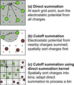
Figure 13.3 Cutoff summation algorithm.
In practice, we know that each grid point needs to receive contributions from atoms that are close to it. The atoms that are far away from a grid point will have negligible contribution to the energy value at the grid point because the contribution is inversely proportional to the distance. Figure 13.3(b) illustrates this observation with a circle drawn around a grid point. The contributions to the grid point energy from atoms outside the circle (maroon) are negligible. If we can devise an algorithm where each grid point only receives contributions from atoms within a fixed radius of its coordinate (green), the computational complexity of the algorithm would be reduced to linearly proportional to the volume of the system. This would make the computation time of the algorithm linearly proportional to the volume of the system. Such algorithms have been used extensively in sequential computation.
In sequential computing, a simple cutoff algorithm handles one atom at a time. For each atom, the algorithm iterates through the grid points that fall within a radius of the atom’s coordinate. This is a straightforward procedure since the grid points are in an array that can be easily indexed as a function of their coordinates. However, this simple procedure does not carry easily to parallel execution. The reason is what we discussed in Section 13.2: the atom-centric decomposition does not work well due to it scatter memory access behavior. However, as we discussed in Chapter 9, it is important that a parallel algorithm matches the work efficiency of an efficient sequential algorithm.
Therefore, we need to find a cutoff binning algorithm based on the grid-centric decomposition: each thread calculates the energy value at one grid point. Fortunately, there is a well-known approach to adapting the direct summation algorithm, such as the one in Figure 12.9, into a cutoff binning algorithm. Rodrigues et al. present such an algorithm for the electrostatic potential problem [RSH 2008].
The key idea of the algorithm is to first sort the input atoms into bins according to their coordinates. Each bin corresponds to a box in the grid space and it contains all atoms of which the coordinate falls into the box. We define a “neighborhood” of bins for a grid point to be the collection of bins that contain all the atoms that can contribute to the energy value of a grid point. If we have an efficient way of managing neighborhood bins for all grid points, we can calculate the energy value for a grid point by examining the neighborhood bins for the grid point. This is illustrated in Figure 13.3(c). Although Figure 13.3(c) shows only one layer (2D) of bins that immediately surround that containing a grid point as its neighborhood, a real algorithm will typically have multiple layers (3D) of bins in a grid’s neighborhood. In this algorithm, all threads iterate through their own neighborhood. They use their block and thread indices to identify the appropriate bins. Note that some of the atoms in the surrounding bins may not fall into the radius. Therefore, when processing an atom, all threads need to check if the atom falls into its radius. This can cause some control divergence among threads in a warp.
The main source of improvement in work efficiency comes from the fact that each thread now examines a much smaller set of atoms in a large grid system. This, however, makes constant memory much less attractive for holding the atoms. Since thread blocks will be accessing different neighborhoods, the limited-size constant memory will unlikely be able to hold all the atoms that are needed by all active thread blocks. This motivates the use of global memory to hold a much larger set of atoms. To mitigate the bandwidth consumption, threads in a block collaborate in loading the atom information in the common neighborhood into the shared memory. All threads then examine the atoms out of shared memory. Readers are referred to Rodrigues et al. [RHS2008] for more details of this algorithm.
One subtle issue with binning is that bins may end up with a different number of atoms. Since the atoms are statistically distributed in the grid system, some bins may have lots of atoms and some bins may end up with no atom at all. To guarantee memory coalescing, it is important that all bins are of the same size and aligned at appropriate coalescing boundaries. To accommodate the bins with the largest number of atoms, we would need to make the size of all other bins the same size. This would require us to fill many bins with dummy atoms of which the electrical charge is 0, which causes two negative effects. First, the dummy atoms still occupy global memory and shared memory storage. They also consumer data transfer bandwidth to the device. Second, the dummy atoms extend the execution time of the thread blocks of which the bins have few real atoms.
A well-known solution is to set the bin size at a reasonable level, typically much smaller than the largest possible number of atoms in a bin. The binning process maintains an overflow list. When processing an atom, if the atom’s home bin is full, the atom is added to the overflow list instead. After the device completes a kernel, the result grid point energy values are transferred back to the host. The host executes a sequential cutoff algorithm on the atoms in the overflow list to complete the missing contributions from these overflow atoms. As long as the overflow atoms account for only a small percentage of the atoms, the additional sequential processing time of the overflow atoms is typically shorter than that of the device execution time. One can also design the kernel so that each kernel invocation calculates the energy values for a subvolume of grid points. After each kernel completes, the host launches the next kernel and processes the overflow atoms for the completed kernel. Thus, the host will be processing the overflow atoms while the device executes the next kernel. This approach can hide most if not all the delays in processing overflow atoms since it is done in parallel with the execution of the next kernel.
Figure 13.4 shows a comparison of scalability and performance of the various electrostatic potential map algorithms. Note that the CPU-SSE3 curve is based on a sequential cutoff algorithm. For a map with small volumes, around 1,000 Angstrom3, the host (CPU with SSE) executes faster than the DCS kernel shown in Figure 13.4. This is because there is not enough work to fully utilize a CUDA device for such a small volume. However, for moderate volumes, between 2,000 and 500,000 Angstrom3, the direct summation kernel performs significantly better than the host due to its massive execution. As we anticipated, the direct summation kernel scales poorly when the volume size reaches about 1,000,000 Angstrom3, and runs longer than the sequential algorithm on the CPU! This is due to the fact that the algorithm complexity of the DCS kernel is higher than the sequential algorithm and thus the amount of work done by the kernel grows much faster than that done by the sequential algorithm. For a volume size larger than 1,000,000 Angstrom3, the amount of work is so large that it swamps the hardware execution resources.
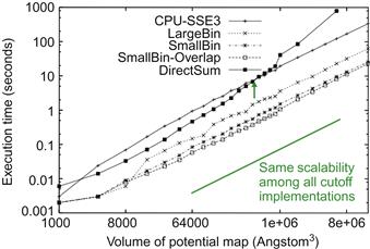
Figure 13.4 Scalability and performance of difference algorithms for calculating an electrostatic potential map.
Figure 13.4 also shows the running time of three binned cutoff algorithms. The LargeBin algorithm is a straightforward adaptation of the DCS kernel for the cutoff. The kernel is designed to process a subvolume of the grid points. Before each kernel launch, the CPU transfers all atoms that are in the combined neighborhood of all the grid points in the subvolume. These atoms are still stored in the constant memory. All threads examine all atoms in the joint neighborhood. The advantage of the kernel is its simplicity. It is essentially the same as the direct summation kernel with a relatively large, preselected neighborhood of atoms. Note that the LargeBin approach performs reasonably well for moderate volumes and scales well for large volumes.
The SmallBin algorithm allows the threads running the same kernel to process a different neighborhood of atoms. This is the algorithm that uses global memory and shared memory for storing atoms. The algorithm achieves higher efficiency than the LargeBin algorithm because each thread needs to examine a smaller number of atoms. For moderate volumes, around 8,000 Angstrom3, the LargeBin algorithm slightly outperforms the SmallBin algorithm. The reason is that the SmallBin algorithm does incur more instruction overhead for loading atoms from global memory into shared memory. For a moderate volume, there is a limited number of atoms in the entire system. The ability to examine a smaller number of atoms does not provide sufficient advantage to overcome the additional instruction overhead. However, the difference is so small at 8,000 Angstrom3 that the SmallBin algorithm is still a clear win across all volume sizes. The SmallBin-Overlap algorithm overlaps the sequential overflow atom processing with the next kernel execution. It provides a slight but noticeable improvement in running time over the SmallBin algorithm. The SmallBin–Overlap algorithm achieves a 17× speedup over an efficiently implemented sequential CPU-SSE cutoff algorithm, and maintains the same scalability for large volumes.
13.4 Computational Thinking
Computational thinking is arguably the most important aspect of parallel application development [Wing2006]. We define computational thinking as the thought process of formulating domain problems in terms of computation steps and algorithms. Like any other thought processes and problem-solving skills, computational thinking is an art. As we mentioned in Chapter 1, we believe that computational thinking is best taught with an iterative approach where students bounce back and forth between practical experience and abstract concepts.
The electrostatic potential map kernels used in Chapter 12 and this chapter serve as good examples of computational thinking. To develop an efficient parallel application that solves the electrostatic potential map problem, one must come up with a good high-level decomposition of the problem. As we showed in Section 13.2, one must have a clear understanding of the desirable (e.g., gather in CUDA) and undesirable (e.g., scatter in CUDA) memory access behaviors to make a wise decision.
Given a problem decomposition, parallel programmers face a potentially overwhelming task of designing algorithms to overcome major challenges in parallelism, execution efficiency, and memory bandwidth consumption. There is a very large volume of literature on a wide range of algorithm techniques that can be hard to understand. It is beyond the scope of this book to have a comprehensive coverage of the available techniques. We did discuss a substantial set of techniques that have broad applicability. While these techniques are based on CUDA, they help readers build up the foundation for computational thinking in general. We believe that humans understand best when we learn from the bottom up. That is, we first learn the concepts in the context of a particular programming model, which provides us with solid footing before we generalize our knowledge to other programming models. An in-depth experience with the CUDA model also enables us to gain maturity, which will help us learn concepts that may not even be pertinent to the CUDA model.
There is a myriad of skills needed for a parallel programmer to be an effective computational thinker. We summarize these foundational skills as follows:
• Computer architecture: memory organization, caching and locality, memory bandwidth, SIMT versus SPMD versus SIMD execution, and floating-point precision versus accuracy. These concepts are critical in understanding the trade-offs between algorithms.
• Programming models and compilers: parallel execution models, types of available memories, array data layout, and thread granularity transformation. These concepts are needed for thinking through the arrangements of data structures and loop structures to achieve better performance.
• Algorithm techniques: tiling, cutoff, scatter–gather, binning, and others. These techniques form the toolbox for designing superior parallel algorithms. Understanding the scalability, efficiency, and memory bandwidth implications of these techniques is essential in computational thinking.
• Domain knowledge: numerical methods, precision, accuracy, and numerical stability. Understanding these ground rules allows a developer to be much more creative in applying algorithm techniques.
Our goal for this book is to provide a solid foundation for all the four areas. Readers should continue to broaden their knowledge in these areas after finishing this book. Most importantly, the best way of building up more computational thinking skills is to keep solving challenging problems with excellent computational solutions.
13.5 Summary
In summary, we have discussed the main dimensions of algorithm selection and computational thinking. The key lesson is that given a problem decomposition decision, programmers will typically have to select from a variety of algorithms. Some of these algorithms achieve different trade-offs while maintaining the same numerical accuracy. Others involve sacrificing some level of accuracy to achieve much more scalable running times. The cutoff strategy is perhaps the most popular of such strategies. Even though we introduced cutoff in the context of electrostatic potential map calculation, it is used in many domains including ray tracing in graphics and collision detection in games. Computational thinking skills allow an algorithm designer to work around the roadblocks and reach a good solution.
13.6 Exercises
13.1 Write a host function to perform binning of atoms. Determine the representation of the bins as arrays. Think about coalescing requirements. Make sure that every thread can easily find the bins it needs to process.
13.2 Write the part of the cutoff kernel function that determines if an atom is in the neighborhood of a grid point based on the coordinates of the atoms and the grid points.
References
1. Message Passing Interface Forum, MPI—A Message Passing Interface Standard Version 2.2, Available at: <http://www.mpi-forum.org/docs/mpi-2.2/mpi22-report.pdf>, 04.09.09.
2. Mattson TG, Sanders BA, Massingill BL. Patterns of Parallel Programming Reading, MA: Addison-Wesley Professional; 2004.
3. Rodrigues, C. I., Stone, J., Hardy, D., Hwu, W. W.GPU Acceleration of Cutoff-Based Potential Summation. ACM Computing Frontier Conference 2008, Italy: May 2008.
4. Wing J. Computational thinking. Communications of the ACM. 2006;49 pp. 33–35.