3.3.4 Development of the Kinematic Trajectory-Tracking Error Model
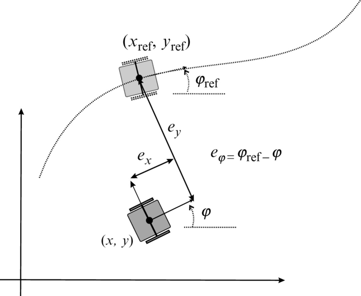
In order to solve the control problem the transformation of robot coordinates is often performed on the form that is better suited for control purposes. The posture of the error is not given in the global coordinate system, but rather as an error in the local coordinate system of the robot that is aligned with the driving mechanism. This error is expressed as the deviation between a virtual reference robot and the actual robot as depicted in Fig. 3.21. The obtained errors are as follows: ex that gives the error in the direction of driving, ey that gives the error in the perpendicular direction, and eφ that gives the error in the orientation. These errors are illustrated in Fig. 3.21. The approach was first adopted in [8].
The posture error ![]() is determined using the actual posture
is determined using the actual posture ![]() of the real robot and the reference posture
of the real robot and the reference posture ![]() of the virtual reference robot:
of the virtual reference robot:
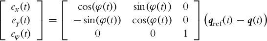
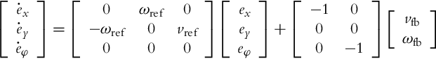
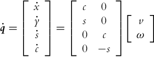
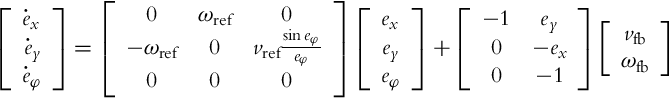
Assuming that the actual and the reference robot have the same kinematic model given by Eq. (2.2) and taking into account the transformation (3.35), the posture error model can be written as follows:

where vref and ωref are the linear and the angular reference velocities given by Eqs. (3.22), (3.23). The input ![]() is to be commanded by the controller. Very often [9] the control u is decomposed as
is to be commanded by the controller. Very often [9] the control u is decomposed as
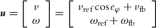
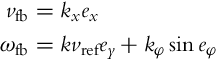
where vfb and ωfb are the feedback signals to be defined later, while ![]() and ωref are the feedforward signals, although technically speaking,
and ωref are the feedforward signals, although technically speaking, ![]() is modulated with the orientation error that originates from the output. On the other hand, when the orientation error is driven to 0,
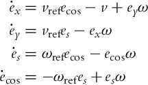
is modulated with the orientation error that originates from the output. On the other hand, when the orientation error is driven to 0, ![]() becomes a “true” feedforward. Inserting the control (3.37) into Eq. (3.36) results in the tracking-error model:
becomes a “true” feedforward. Inserting the control (3.37) into Eq. (3.36) results in the tracking-error model:

The control goal is to drive the errors of the error model (3.38) toward 0 by appropriately choosing the controls vfb and ωfb. This is the topic of the following sections.
3.3.5 Linear Controller
The error model (3.38) is nonlinear. In this section this model will be linearized to enable the use of a linear controller. The linearization has to take place around some equilibrium point. Here the obvious choice is the zero error (ex = ey = 0, eφ = 0). This point is an equilibrium point of Eq. (3.38) if both feedback velocities are also 0 (vfb = 0, ωfb = 0). Linearizing Eq. (3.38) around the zero-error yields the following:
which is a linear time-varying system due to vref(t) and ωref(t) being time dependent.
The system given by Eq. (3.39) is a state-space representation of a dynamic error-system where all the states (errors in this case) are accessible. A full state feedback is therefore possible if the system is controllable. If it is assumed that vref and ωref are constant (the reference path consists of straight line segments and circular arcs), it is easy to confirm that the controllability matrix defined by Eq. (3.28) is of the full rank, and consequently all the errors can be forced to 0 by a static state feedback. If vref and ωref are not constant, controllability is retained if either of the reference signals is different from 0, although the analysis becomes more complicated.
Due to a special structure of the system (3.39), a static state feedback with a simple form of gain matrix is often used:
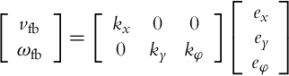
We see that the error in the direction of driving is corrected by vfb, while the errors in the orientation and in the lateral directions are corrected by ωfb.
Controller gains (kx, ky, kφ) can be determined by trial and error, by optimizing them on a system model, by using the pole placement approach, etc. Here, the control gains are chosen such that the poles of the control system lie in appropriate locations in the complex plane s. The system has three poles of which one has to be real while the other two will be conjugate complex. First, the poles will be placed on fixed locations − 2ζωn, and ![]() where the undamped natural frequency ωn > 0 and the damping coefficient 0 < ζ < 1 are designer parameters. If the characteristic polynomial of the closed-loop system
where the undamped natural frequency ωn > 0 and the damping coefficient 0 < ζ < 1 are designer parameters. If the characteristic polynomial of the closed-loop system

is compared to the desired one,
the solution for control gains can be obtained [6]:

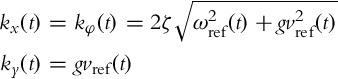
Note that ωn should be larger than the maximum of |ωref(t)|. Control gains given by Eq. (3.41) are not practically applicable because ky(t) becomes extremely large when the reference velocity vref(t) is low. To overcome this problem, the undamped natural frequency ωn will become time-varying. Since it is natural to adapt the transient response settling times to the reference velocities, the following choice seems sensible: ![]() , g > 0. Repeating a similar procedure as above, the following control gains are obtained:
, g > 0. Repeating a similar procedure as above, the following control gains are obtained:
Two remarks are important in the context of control algorithms shown in this section:
• The control laws are designed based on the linearized models. A linearized model is only valid in the vicinity of the operating point (zero error in this case), and the control performance might not be as expected in case of large control errors.
• Even if we deal with a linear but time-varying system, some of the results known from linear time invariant systems are no longer valid. Here we should mention that even if all the poles lie in the (fixed) locations of the left half-plane of the complex plane s, the system might be unstable.
In spite of the potential difficulties mentioned above, linear control laws are often used in practice due to their simplicity, relatively easy tuning, and acceptable performance and robustness. A simulated example of the use is given below.
Example 3.9
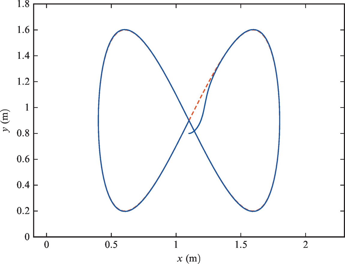
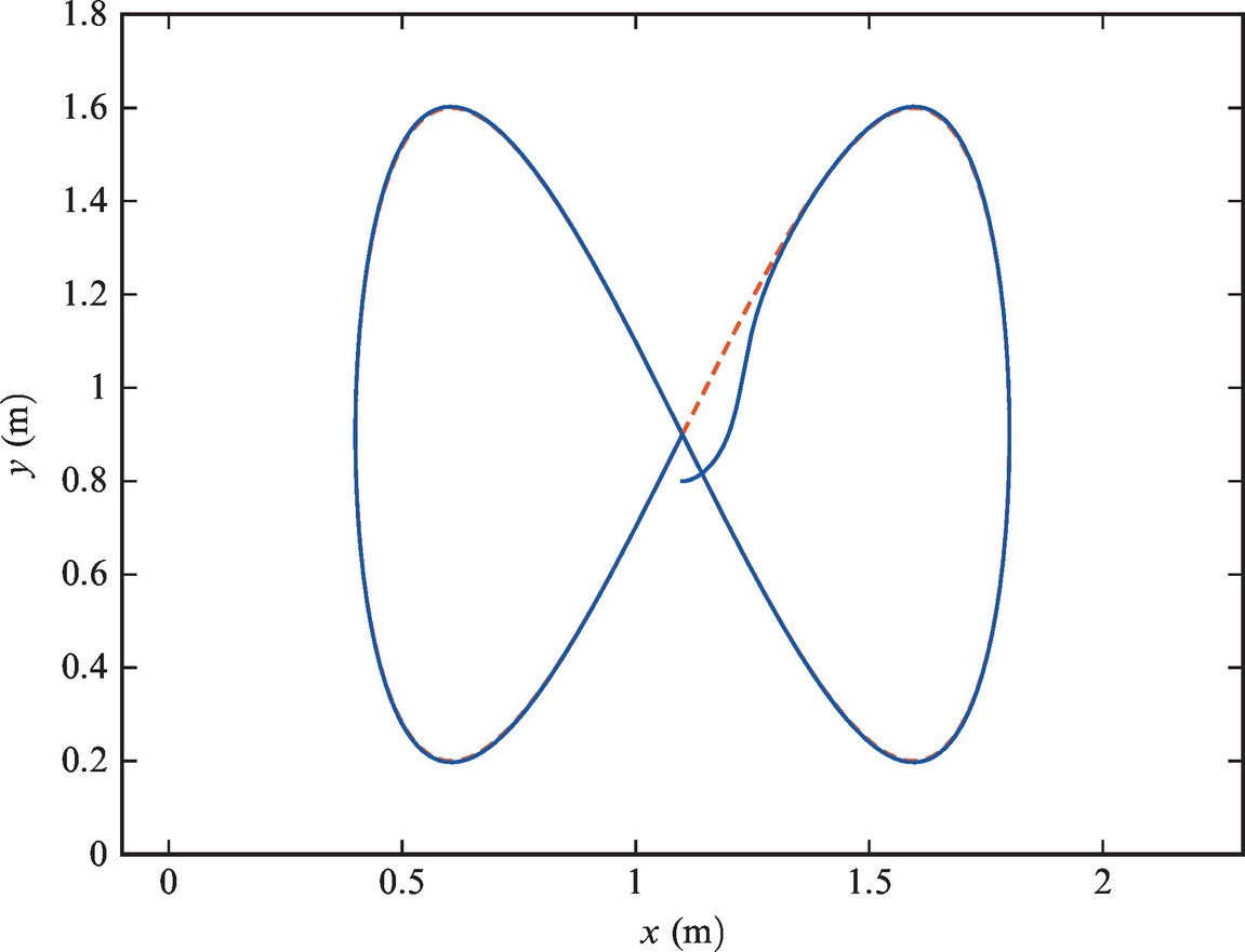
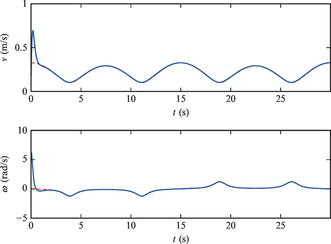
A differentially driven vehicle is to be controlled to follow the reference trajectory ![]() and
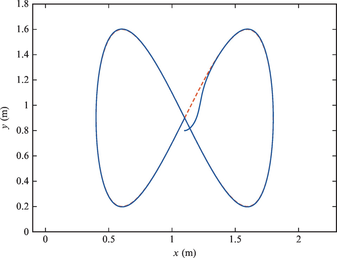
and ![]() . Sampling time is Ts = 0.033 s. The initial pose is [x(0), y(0), φ(0)] = [1.1, 0.8, 0]. Implement the algorithm presented in this section with the control gains given by Eq. (3.41) in a Matlab code and show the graphical results.
. Sampling time is Ts = 0.033 s. The initial pose is [x(0), y(0), φ(0)] = [1.1, 0.8, 0]. Implement the algorithm presented in this section with the control gains given by Eq. (3.41) in a Matlab code and show the graphical results.
Solution
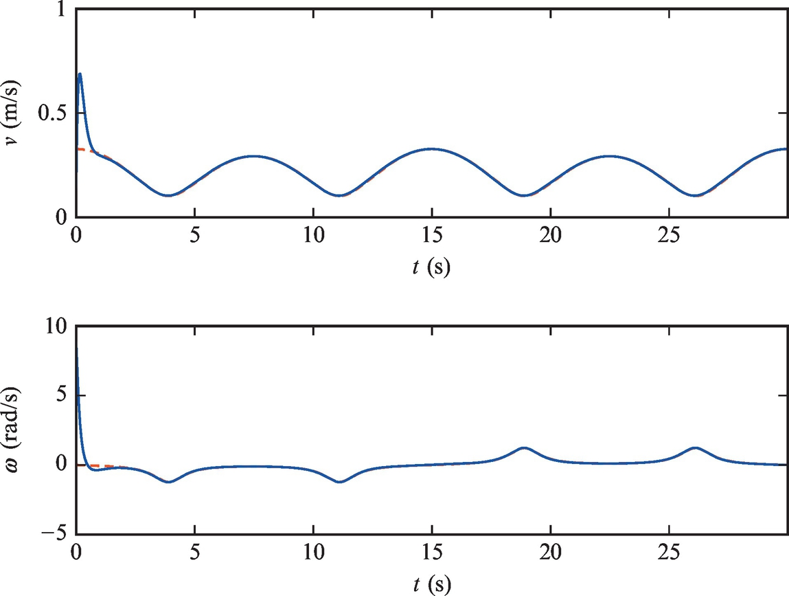
The code is given in Listing 3.8. Simulation results are shown in Figs. 3.22 and 3.23 where good tracking can be observed.
3.3.6 Lyapunov-Based Control Design
We have already mentioned that the error model (3.38) is inherently nonlinear. Nonlinear systems are best controlled using a nonlinear controller that takes into account all the properties of the original system during control design. Theory based on Lyapunov functions is often used for nonlinear system stabilization problems. In our case, the (asymptotic) stability of the error model (3.38) will be analyzed in the presence of different control laws.
Lyapunov Stability
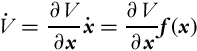
The second method of Lyapunov will be introduced briefly. The method gives sufficient conditions for (asymptotic) stability of equilibrium points of a nonlinear dynamical system given by ![]() ,
, ![]() . First, it is assumed that the equilibrium lies at x = 0. The approach is based on positive definite scalar functions
. First, it is assumed that the equilibrium lies at x = 0. The approach is based on positive definite scalar functions ![]() that fulfill the following: V (x) = 0 if x = 0, and V (x) > 0 if x≠0. The stability of the equilibrium point is analyzed by checking the derivative of the function V. It is very important that the derivative is obtained along the solutions of the differential equation of the system:
that fulfill the following: V (x) = 0 if x = 0, and V (x) > 0 if x≠0. The stability of the equilibrium point is analyzed by checking the derivative of the function V. It is very important that the derivative is obtained along the solutions of the differential equation of the system:
If ![]() (
(![]() is negative semidefinite), the equilibrium is (locally) stable. If
is negative semidefinite), the equilibrium is (locally) stable. If ![]() except at x = 0 (
except at x = 0 (![]() is negative definite), the equilibrium is (locally) asymptotically stable. If
is negative definite), the equilibrium is (locally) asymptotically stable. If ![]() , the results are global. The approach is therefore based on searching for the functions with the above properties that are referred to as Lyapunov functions. Very often a quadratic Lyapunov function candidate is chosen, and if we are able to show its derivative is negative or at least zero, stability of the system is concluded.
, the results are global. The approach is therefore based on searching for the functions with the above properties that are referred to as Lyapunov functions. Very often a quadratic Lyapunov function candidate is chosen, and if we are able to show its derivative is negative or at least zero, stability of the system is concluded.
A classical interpretation of Lyapunov functions is based on the system energy point of view. If system energy is used as a Lyapunov function, and the system is dissipative, the energy in the system cannot increase (the derivative of the function is nonpositive). Consequently, all the signals remain bounded, and the system stability can be confirmed. But it needs to be stressed that a Lyapunov function might not be related to system energy. Above all, “system stability” is an incorrect term in the nonlinear framework. Rather, stability of equilibrium points, or more generally of invariant sets, is to be analyzed. It is easy to find the systems where stable and unstable equilibria coexist.
Control Design in the Lyapunov Stability Framework
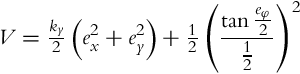
We shall show in the following how the Lyapunov stability theorem can be used for control design purposes. Our nonlinear system (3.38) has three states with equilibrium points at e = 0. We would like to design a control that would make this point stable and if possible asymptotically stable, which means that all the trajectories would eventually converge to the reference trajectory and stay there forever. The most obvious Lyapunov function candidate is a sum of three squared errors:
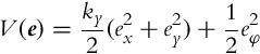
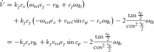
which can be interpreted as a weighted sum of the squared error in distance and the squared error in orientation. A positive constant ky has to be added because of different units, but it will later be shown that this constant plays an important role in the control law design. The time derivative of V is
but this derivative has to be evaluated along the solutions of Eq. (3.38), which means that the error derivatives from Eq. (3.38) should be introduced

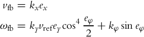
The idea of Lyapunov-based control design is to make the derivative of the Lyapunov function negative by choosing the control laws properly. It is therefore obvious how the control could be constructed in this case. The linear velocity vfb will make the first term on the right-hand side in Eq. (3.46) negative (by completing it to the negative square), while the angular velocity ωfb will cancel the second term in Eq. (3.46) and will make the third one negative (by completing it to the negative square). The control law that achieves that is
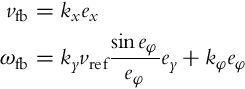
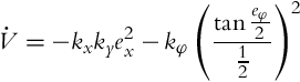
This control law is a known and well-established control law from the literature [6, 10]. Now introducing the proposed control (3.47), ![]() becomes
becomes
Control gains are positive, and it will later be shown that kx and kφ can be arbitrary, uniformly continuous positive functions, while ky is required to be a positive constant. The derivative of the Lyapunov function is clearly nonpositive, but since it is evaluated to zero at ex = 0, eφ = 0, irrespective of ey, the derivative is negative semidefinite, and the equilibrium is stable. This result means that the error will stay bounded, but its convergence to 0 has not been proven.
The analysis of error convergence is considerably more difficult. In order to cope with it, we first need to introduce some additional mathematical tools. Signal norms will play an important role. The ![]() norm of a function x(t) is defined as
norm of a function x(t) is defined as
where |⋅| is the vector (scalar) length. If the above integral exists (is finite), the function x(t) is said to belong to ![]() . Limiting p toward infinity provides a very important class of functions
. Limiting p toward infinity provides a very important class of functions ![]() : bounded functions.
: bounded functions.
Two very well-known lemmas will be used to prove the stability of control laws. The first one is Barbălat’s lemma and the other one is a derivation of Barbălat’s lemma. Both lemmas are taken from [11] and are given below for the sake of completeness.
Lemma 3.1
(Barbălat’s Lemma)
If ![]() exists and is finite, and f(t) is a uniformly continuous function, then
exists and is finite, and f(t) is a uniformly continuous function, then ![]() .
.
Lemma 3.2
If ![]() and
and ![]() for some
for some ![]() , then f(t) → 0 as
, then f(t) → 0 as ![]() .
.
Now, we are ready to address the problem of convergence of the errors in Eq. (3.38). Due to Eq. (3.48), ![]() , and therefore the Lyapunov function is nonincreasing and thus has the limit
, and therefore the Lyapunov function is nonincreasing and thus has the limit ![]() . Consequently, the states of Eq. (3.38) are bounded:
. Consequently, the states of Eq. (3.38) are bounded:
Additionally, it follows from Eq. (3.47) that the control signals are bounded, and from Eq. (3.38) that the derivatives of the errors are bounded:
where we also took into account that vref, ωref, kx, and kφ are bounded. The latter is true in the case of smooth reference trajectories (xref, yref, φref).
In order to show asymptotic stability of Eq. (3.38), let us first calculate the following integral of ![]() from Eq. (3.48):
from Eq. (3.48):
Since V is a positive definite function, the following inequality holds:

where the lower bounds of functions kx(t) and kφ(t) have been introduced:

It follows from Eq. (3.53) that the errors ex(t) and eφ(t) belong to ![]() . Based on Lemma 3.2 it is easy to show that the errors ex(t) and eφ(t) converge to 0. Since the limit
. Based on Lemma 3.2 it is easy to show that the errors ex(t) and eφ(t) converge to 0. Since the limit ![]() exists, then also
exists, then also ![]() exists.
exists.
We have seen that the convergence of the errors ex(t) and eφ(t) to 0 is relatively simple to show and the conditions for convergence are relatively mild—control gains and reference trajectories have to be bounded. Convergence of ey to 0 is more difficult to show, and the requirements are much more difficult to achieve, as is shown next. Besides the control gains being uniformly continuous, the reference velocities have to be persistently exciting, which means that either vref or ωref should not limit to 0. Two cases will therefore be distinguished. In the first one, ![]() will be assumed, and in the second,
will be assumed, and in the second, ![]() will be assumed.
will be assumed.
Now, it will be assumed that ![]() . Applying Lemma 3.1 on
. Applying Lemma 3.1 on ![]() from Eq. (3.38) ensures that
from Eq. (3.38) ensures that ![]() since
since ![]() exists and is finite and
exists and is finite and ![]() is uniformly continuous. The latter is true due to Eq. (3.38) if ωfb is uniformly continuous. The easiest way to check the uniform continuity of f(t) on
is uniformly continuous. The latter is true due to Eq. (3.38) if ωfb is uniformly continuous. The easiest way to check the uniform continuity of f(t) on ![]() is to see if
is to see if ![]() . It has already been shown that ey and eφ are uniformly continuous, while the control gain kφ and the reference velocity vref are uniformly continuous by the assumption, so it follows from Eq. (3.47) that
. It has already been shown that ey and eφ are uniformly continuous, while the control gain kφ and the reference velocity vref are uniformly continuous by the assumption, so it follows from Eq. (3.47) that ![]() is also uniformly continuous. The statement
is also uniformly continuous. The statement ![]() (which is identical to
(which is identical to ![]() ) has therefore been proven. The convergence of ey to 0 follows from Eq. (3.47):
) has therefore been proven. The convergence of ey to 0 follows from Eq. (3.47):
Now, it will be assumed that ![]() . Again one has to guarantee that
. Again one has to guarantee that ![]() . This is true if vref and kφ are uniformly continuous, as shown before. Then Barbălat’s lemma (Lemma 3.1) is applied on
. This is true if vref and kφ are uniformly continuous, as shown before. Then Barbălat’s lemma (Lemma 3.1) is applied on ![]() in Eq. (3.38). It has already been shown that ex, ey, and ωfb are uniformly continuous; vfb is uniformly continuous since kx is uniformly continuous by the assumption; and ωref is also continuous from the assumption of this paragraph. This proves the statement
in Eq. (3.38). It has already been shown that ex, ey, and ωfb are uniformly continuous; vfb is uniformly continuous since kx is uniformly continuous by the assumption; and ωref is also continuous from the assumption of this paragraph. This proves the statement ![]() . Like in the last paragraph, it can be concluded that the last two terms in Eq. (3.38) for
. Like in the last paragraph, it can be concluded that the last two terms in Eq. (3.38) for ![]() go to 0 as t goes to infinity. Consequently, the product ωrefey also goes to 0. Since ωref is persistently exciting and does not go to 0, ey has to go to 0.
go to 0 as t goes to infinity. Consequently, the product ωrefey also goes to 0. Since ωref is persistently exciting and does not go to 0, ey has to go to 0.
Once again it should be stressed that for convergence of ex and eφ, only boundedness of vref or ωref is required. A considerably more difficult task is to drive ey to 0. This is achieved by persistent excitation from either vref or ωref. All the results are valid globally, which means that the convergence is guaranteed irrespective of the initial pose.
Example 3.10
A differentially driven vehicle is to be controlled to follow the reference trajectory ![]() and
and ![]() . Sampling time is Ts = 0.033 s. The initial pose is [x(0), y(0), φ(0)] = [1.1, 0.8, 0]. Implement the control algorithm presented in this section in a Matlab code, experiment with control gains, and show the graphical results.
. Sampling time is Ts = 0.033 s. The initial pose is [x(0), y(0), φ(0)] = [1.1, 0.8, 0]. Implement the control algorithm presented in this section in a Matlab code, experiment with control gains, and show the graphical results.
Solution
The code is given in Listing 3.9. Simulation results of Example 3.10 are shown in Figs. 3.24 and 3.25 where good tracking can be observed. Note that any positive functions can be used for kx(t) and kφ(t). Here the functions that are chosen make the linearized model of the system the same as in the case of the linear tracking controller (Example 3.9). Control laws are not the same, but they become the same in the limit case (![]() ). The result of this choice is that the shape of transients is the same near the reference trajectory irrespective of the reference velocities.
). The result of this choice is that the shape of transients is the same near the reference trajectory irrespective of the reference velocities.

Periodic Control Law Design
The problem of tracking is clearly periodic with respect to the orientation. This can be observed from the kinematic model by using an arbitrary control input and an arbitrary initial condition, resulting in a certain robot trajectory. If the same control input is applied to the robot and the initial condition only differs from the previous one by a multiple of 2π, the same response is obtained for x(t) and y(t), while φ(t) differs from the previous solution for the same multiple of 2π. The periodic nature should also be reflected in the control law used for the tracking. This should mean that one searches for a control law that is periodic with respect to the error in the orientation eφ (the period is 2π) and ensures the convergence of the posture error e to one of the points ![]() . Thus, all the usual problems with orientation mapping to the (−π, π] are alleviated. These problems can become critical around ±180 degree in certain applications, for example, when using an observer to estimate the robot pose from the delayed measurements. Note that certain control laws are periodic in the sense discussed above, for example, feedback linearization control law given by Eqs. (3.25), (3.34) is periodic.
. Thus, all the usual problems with orientation mapping to the (−π, π] are alleviated. These problems can become critical around ±180 degree in certain applications, for example, when using an observer to estimate the robot pose from the delayed measurements. Note that certain control laws are periodic in the sense discussed above, for example, feedback linearization control law given by Eqs. (3.25), (3.34) is periodic.
Obviously, the functions that are used in the section for the convergence analysis should also be periodic in eφ. This means that these functions have multiple local minima and therefore do not satisfy the properties of the classic Lyapunov functions. Although the stability analysis resembles Lyapunov’s direct method (the second method of Lyapunov), the convergence is not proven by this stability theory because the convergence of e to zero is not needed in our approach. Nevertheless, the functions used in this section for the convergence analysis will still be referred to as “Lyapunov functions.”
Our goal is to bring the position error to zero, while the orientation error should converge to any multiple of 2π. In order to do this, a Lyapunov function that is periodic with respect to eφ (with a natural period of 2π) will be used. First, the concept will be shown on one Lyapunov function, and later this will be extended to a more general case. The first Lyapunov-function candidate is chosen as
where ky is a positive constant. Its derivative along the solutions of Eq. (3.38) is the following:
If the following control law is applied
where kx and kφ are positive bounded functions, the derivative ![]() from Eq. (3.57) becomes
from Eq. (3.57) becomes
Following the same lines as in the analysis of the control law (3.47) it can easily be concluded that ex and ![]() converge to 0 (this means that
converge to 0 (this means that ![]() ,
, ![]() ) in the case of bounded control gains and a bounded trajectory. The convergence of ey to 0 can also be concluded after a lengthy analysis if the same conditions are met as in the case of the control law (3.47).
) in the case of bounded control gains and a bounded trajectory. The convergence of ey to 0 can also be concluded after a lengthy analysis if the same conditions are met as in the case of the control law (3.47).
Example 3.11
A differentially driven vehicle is to be controlled to follow the reference trajectory ![]() and
and ![]() . Sampling time is Ts = 0.033 s. The initial pose is [x(0), y(0), φ(0)] = [1.1, 0.8, 0]. Implement the control algorithm presented in this section in a Matlab code, experiment with control gains, and show the graphical results.
. Sampling time is Ts = 0.033 s. The initial pose is [x(0), y(0), φ(0)] = [1.1, 0.8, 0]. Implement the control algorithm presented in this section in a Matlab code, experiment with control gains, and show the graphical results.
Solution
The code is given in Listing 3.10. Simulation results are shown in Figs. 3.26 and 3.27, where good tracking can be observed.
A well-known control law by Kanayama et al. [9] can also be analyzed in the proposed framework. Choosing the Lyapunov function as

and using the control law proposed in [9] (there was also a third factor |vref| in the second term of ωfb that can also be included in kφ),
results in a stable error-system where the convergence of all the errors can be shown under the same conditions as before. Note that beside stable equilibria at eφ = 2kπ, ![]() , there is also an unstable or repelling equilibrium at eφ = (2k + 1)π,
, there is also an unstable or repelling equilibrium at eφ = (2k + 1)π, ![]() .
.
A framework for periodic control law design is presented in [12]. Perhaps it is worth mentioning that it is quite simple to extend the proposed techniques to the control design for symmetric vehicles that can move in the forward and the backward direction during normal operation. In this case Lyapunov functions should be periodic with a period of π on eφ.
Four-State Error Model of the System
In this section we will tackle the same problem as in the previous section, that is, from the control point of view we often want to track any robot pose that is different from the reference one for a multiple of 360 degree. The model (3.38) does not make this problem easier because the orientation error should be usually driven to 0 using Eq. (3.38). In this section a kinematic model of the system is presented where all the poses that differ in orientation for a multiple of 360 degree are presented as one. This can be achieved by extended the state vector for one element. The variable φ(t) from the original kinematic model (2.2) is exchanged by two new variables, ![]() and
and ![]() . Their derivatives are
. Their derivatives are
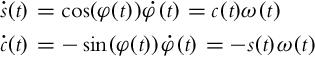
The new kinematic model is then obtained:
The new error states are defined as follows:

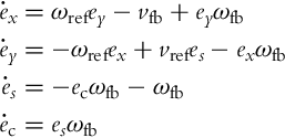
After the differentiation of Eq. (3.64) and some manipulations, the following system is obtained:
Like in Eq. (3.37), v = vrefecos + vfb and ω = ωref + ωfb will be used in the control law. The control goal is to drive ex, ey, and es to 0. The variable ecos is obtained as the cosine of the error in the orientation and should be driven to 1. This is why a new error will be defined as ec = ecos − 1 and the final error model of the system is now
A controller that achieves asymptotic stability of the error model (3.66) will be developed based on a Lyapunov approach. A very straightforward idea would be to use a Lyapunov function of the type
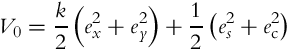
Interestingly, this Lyapunov function results in the control law (3.61). However, a slightly more complex function will be proposed here, which also includes the function (3.67) as a special case. The following Lyapunov-function candidate is proposed to achieve the control goal:

where k > 0 and a > 2 are constants. Note that the range of the function ![]() is [−2, 0], and therefore
is [−2, 0], and therefore
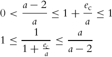
Due to Eq. (3.69) the function V in Eq. (3.68) is lower-bounded by the function V0 in Eq. (3.67), and V fulfills the conditions for the Lyapunov function. The role of ![]() will be explained later on. The function V can be simplified by using the following:
will be explained later on. The function V can be simplified by using the following:
Taking into account the equations of the error model (3.66), (3.70), the derivative of V in Eq. (3.68) is

In order to make ![]() negative semidefinite, the following control law is proposed:
negative semidefinite, the following control law is proposed:

where kx(t) and ks(t) are positive functions, while ![]() . For practical reasons n is a small number (usually − 2, − 1, 0, 1, or 2 are good choices). By taking into account the control law (3.72), the function
. For practical reasons n is a small number (usually − 2, − 1, 0, 1, or 2 are good choices). By taking into account the control law (3.72), the function ![]() becomes
becomes
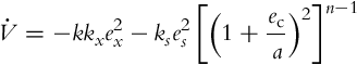
It is again very simple to show the convergence of ex and es based on Eq. (3.73). The convergence of ey and ec is again a little more difficult [13].
Example 3.12
A differentially driven vehicle is to be controlled to follow the reference trajectory ![]() and
and ![]() . Sampling time is Ts = 0.033 s. The initial pose is [x(0), y(0), φ(0)] = [1.1, 0.8, 0]. Implement the control algorithm presented in this section in a Matlab code. Experiment with control gains and additional control design parameters (a and n).
. Sampling time is Ts = 0.033 s. The initial pose is [x(0), y(0), φ(0)] = [1.1, 0.8, 0]. Implement the control algorithm presented in this section in a Matlab code. Experiment with control gains and additional control design parameters (a and n).
Solution
The code is given in Listing 3.11. Simulation results are shown in Figs. 3.28 and 3.29 where good tracking can be observed.


3.3.7 Takagi-Sugeno Fuzzy Control Design in the LMI Framework
The error model (3.38) is nonlinear, as we have already stressed. Takagi-Sugeno models are known to describe the dynamics of nonlinear systems. In this section the model (3.38) will be rewritten in the form of a Takagi-Sugeno model. This form enables the control design of a parallel distributed compensation (PDC) in the linear matrix inequality (LMI) framework.
Takagi-Sugeno Fuzzy Error Model of a Differentially Driven Wheeled Mobile Robot
The Takagi-Sugeno (or TS) models have their roots in fuzzy logic where the model is given in the form of if-then rules. A TS model can also be represented in a more compact polytopic form [14]:
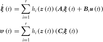
where ![]() is a state vector,
is a state vector, ![]() is an output vector, and
is an output vector, and ![]() is the premise vector depending on the state vector (or some other quantity), Ai, Bi, and Ci are constant matrices. And finally, the nonlinear weighting functions
is the premise vector depending on the state vector (or some other quantity), Ai, Bi, and Ci are constant matrices. And finally, the nonlinear weighting functions ![]() are all nonnegative and such that
are all nonnegative and such that ![]() for an arbitrary z(t). For any nonlinear model, one can find an equivalent fuzzy TS model in a compact region of the state space variable using the sector nonlinearity approach, which consists of decomposing each bounded nonlinear term in a convex combination of its bounds [16]. The number of rules r is then related to the number of the nonlinearities of the model, as shown later.
for an arbitrary z(t). For any nonlinear model, one can find an equivalent fuzzy TS model in a compact region of the state space variable using the sector nonlinearity approach, which consists of decomposing each bounded nonlinear term in a convex combination of its bounds [16]. The number of rules r is then related to the number of the nonlinearities of the model, as shown later.
In this section we will make use of the fact that in the wheeled robot error model the nonlinear functions are known a priori, which makes the use of the aforementioned concept possible. The nonlinear tracking error model (3.38) will therefore be rewritten in the equivalent matrix form:
Four bounded nonlinear functions appear in this model: ωref, ![]() (or with different notation vrsinc(φ)), ey, and ex. The premise vector is therefore:
(or with different notation vrsinc(φ)), ey, and ex. The premise vector is therefore:

First, the controllability of Eq. (3.75) in the linearized sense will be analyzed. It is trivial to see that in the vicinity of the zero-error, the system (3.75) is controllable if vref is different from 0 and |eφ| is different from π, or ωref is different from 0. In practical cases ωref often crosses 0, so vref cannot become 0, and |eφ| cannot become π. The following assumptions are therefore needed to avoid loss of controllability and to restrict our attention to a certain compact region of the error space:
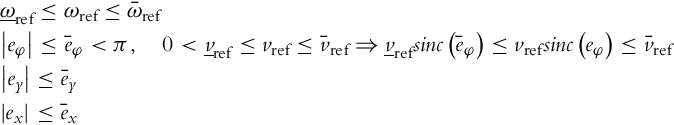
The bounds on vref and ωref are obtained from the actual reference trajectory, while the bounds on the tracking error are selected on the basis of any a priori knowledge available. It is important that these bounds are lower than the error due to measurement noise, initial errors, etc. The bounds from Eq. (3.77) are denoted ![]() and
and ![]() , j = 1, 2, 3, 4. There are four nonlinearities in the system, so the number of fuzzy rules r is equal to 24 = 16. The TS model of Eq. (3.75) is
, j = 1, 2, 3, 4. There are four nonlinearities in the system, so the number of fuzzy rules r is equal to 24 = 16. The TS model of Eq. (3.75) is
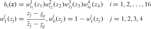
The index i runs in an arbitrary manner through all the vertices of the hypercube defined by Eq. (3.77). The most usual way is to use binary enumeration:

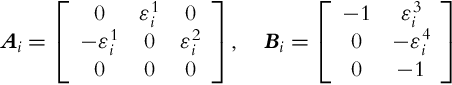
Then ![]() in Eq. (3.79) is defined as:
in Eq. (3.79) is defined as:
And finally the membership functions hi need to be defined:
The TS model (3.78) of the tracking-error model represents the exact model of the system (3.75), that is, in this approach the TS model does not serve as an approximator but takes into account all known nonlinearities that arise in the system. The form Eq. (3.78) is very suitable for the design and analysis tasks as it will be shown in the following.
PDC Control of a Differentially Driven Wheeled Mobile Robot
In order to stabilize the TS model (3.78), a PDC control law [15],
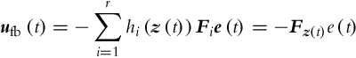
is used. The stabilization problem by using PDC is a well-known one. Due to a specific structure where the plant model and the controller share the same membership functions it is possible to adapt certain tools for linear systems analysis and design to this nonlinear system. Particularly important is the possibility to treat system stability in a formal and straightforward manner. Roughly speaking, the system described by Eqs. (3.78), (3.83) is asymptotically stable if for each i and j the matrix (Ai −BiFj) is Hurwitz (a matrix is Hurwitz if all the eigen values lie in the open left half-plane of the complex plane s). The number of matrices to be analyzed grows very quickly. A systematic approach is therefore needed. It was soon realized that LMIs seem to be a perfect tool for the job [16]. Given the plant parameters in the form of matrices Ai and Bi, it is possible to find the set of controller parameters Fj that asymptotically stabilize the system.
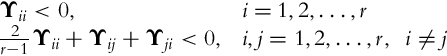
The original approach is too conservative since it does not take into account specific properties of the system, for example, the shape of the membership functions. Many relaxations of the original LMI conditions exist. The adaptation of the result due to [17] is given below: