
Capacitive sensors
Abstract
This chapter starts with resuming the notions capacitance and permittivity. Next, we discuss basic configurations for capacitive sensors. The capacitance value changes with variation in the geometry. The focus is mainly on linear and angular displacement sensors and on force sensors. Next, integrated silicon capacitive sensors are briefly reviewed and some interface circuits are given to measure small capacitance changes. This chapter ends with examples of particular measurement problems where a capacitive sensor forms a suitable solution.
Keywords
Permittivity; capacitance; flat-plate capacitive displacement sensor; silicon capacitive sensors; interfacing; LVDC; level sensors; applications
Capacitive sensors for displacement and force measurements have a number of advantages. A capacitor consists of a pair of conductors; since no other materials are involved, capacitive sensors are very robust and stable, and applicable at high temperatures and in harsh environments. The dimensions of capacitive sensors may vary from extremely small (in Micro-ElectroMechanical Systems, MEMS) up to very large (several meters). The theoretical relation between displacement and capacitance is governed by a simple expression, which in practice can be approximated with high accuracy, resulting in a very high linearity. Using special constructions, the measurement range of capacitive sensors can be extended almost without limit while maintaining the intrinsic accuracy. Moreover, because of the analog nature of the capacitive principle, the sensors have excellent resolution.
This chapter starts with resuming the notions capacitance and permittivity. Next, we discuss basic configurations for capacitive sensors. The capacitance value changes with variation in the geometry. We will focus in particular on linear and angular displacement sensors and on force sensors. Next, integrated silicon capacitive sensors are briefly reviewed and some interface circuits are given to measure small capacitance changes.
5.1 Capacitance and permittivity
The capacitance (or capacity) of an isolated conducting body is defined as Q=C·V, where Q is the charge on the conductor and V is the potential (relative to “infinity,” where the potential is zero by definition). To put it differently, when a charge Q from infinite distance is transferred to the conductor, its potential becomes V=Q/C.
In practice we have a set of conductors instead of just one conductor. When a charge Q is transferred from one conductor to another, the result is a voltage difference V equal to Q/C; the conductors are oppositely charged with Q and −Q, respectively (Fig. 5.1). Again, for this pair of conductors, Q=C·V, where V is the voltage difference between these conductors.

Usually, the capacitance is defined “between” two conductors: this capacitance is determined exclusively by the geometry of the complete set of conductors and the dielectric properties of the (nonconducting) matter in between the conductors and not by the potential of the conductors. The set of conductors is called a capacitor. A well-known configuration is a set of two parallel plates, the flat-plate capacitor, with capacitance
(5.1)
where A is the surface area of the plates and d is the distance between the plates. This is only an approximation: at the plate’s edges the electric field extends outside the space between the plates, resulting in an inhomogeneous field near the edge (stray field or fringe field).
The parameter ε is called the permittivity and describes the dielectric properties of the matter in between the conductors. It is written as the product of ε0, the permittivity of free space or vacuum (about 8.8×10⁻¹² F/m) and εr, the relative permittivity. The latter is also called the dielectric constant of the medium between the conductors. For vacuum εr=1, for air and other gases the dielectric constant is fractionally higher, liquids and solids have larger values (Table 5.1).
Table 5.1
| Material | εr | Material | εr |
|---|---|---|---|
| Vacuum | 1 | Al2O3 | 10 |
| Dry air (0°C, 1 atm) | 1.000576 | SiO2 | 3.8 |
| Water (0°C) | 87.74 | Mica | 5–8 |
| Water (20°C, ω→0) | 80.10 | Teflon | 2.1 |
| Water (20°C, ω→∞) | 4.5–6 | PVC | 3–5 |
| Ice (0°C, ω→0) | 260 | Silicon (20°C) | 11.7 |
| Ice (0°C, ω→∞) | 3.2 | Glass, Pyrex 7740 | 5.00 |

For all kinds of configurations, the capacitance can be calculated [3]. Two straight parallel conductors (Fig. 5.2A) with radius a and centers at spacing d have a capacitance per unit length of:
(5.2)
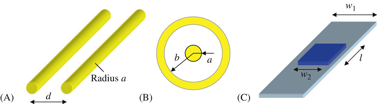
A coaxial cable (two concentric cylinders, Fig. 5.2B) with outer diameter of the central conductor a and inner diameter of the shield b has a capacitance per unit length equal to
(5.3)
The capacitance of other, less symmetrical configurations can be calculated analytically, but results in rather complex expressions [3]. For instance consider a flat-plate capacitor (Fig. 5.2C) with rectangular top electrode (width w2 and length l) opposed to a long strip-electrode (width w1) at distance d. The capacitance of this structure (as often encountered in capacitive displacement sensors) is expressed as follows [4]:
(5.4)
 (5.4)
(5.4)
Anyhow, for a homogeneous dielectric, the capacitance can always be written in the form
(5.5)
where G is a geometric factor. For the parallel plate capacitor with plate distance d and infinite plate dimensions, G=A/d. When the plates have finite dimensions, as for instance for the structure described by Eq. (5.4), G can still be approximated by A/d; we discuss the conditions for this approximation later.
Most capacitive sensors for mechatronic applications are based on changes in the geometric factor G, thereby assuming a constant value of ε. As a fair approximation, the value for the dielectric constant εr of air can be set to 1. At small changes of A or d, however, deviations from this value must be taken into account because the capacitance C changes, using Eq. (5.1) as:
(5.6)
As a matter of fact, ε depends somewhat on the air composition (see for instance [5]):
(5.7)
where pd, pc, and pw are the partial vapor pressure of, respectively, dry air, CO2, and water vapor in mbar. Ad, Ac, Aw, and Bw are empirical parameters, and T is the absolute temperature.
Furthermore, due to relaxation effects, ε appears to be frequency dependent. The dielectric constant is expressed in complex notation: ε=ε′−jε″, where both the real and imaginary parts are frequency dependent. For water the frequency dependency is expressed as [2]:
(5.8)
where τr is the relaxation time. For liquid water at 0°C, τr amounts 17.8×10⁻¹² s, εw(∞)≈5, and εw(0)≈88. In mechatronics we will consider only the static dielectric constant, that is, the value at frequencies far below the relaxation frequency.
Most capacitive displacement sensors operate in air. The influence of atmospheric changes on the dielectric constant can be summarized as follows [5]: starting with standard air (T=293.15 K, pd=100 kPa, pw=117.5 Pa, and pc=30 Pa), the dielectric constant changes by:
Temperature effects can be minimized using balancing techniques (Section 3.2) and proper electrode materials. Humidity cannot be ignored in high precision capacitive displacement sensors; either the temperature should be kept sufficiently far above the dew-point temperature or humidity effects must be avoided through the use of special designs [6].
Many capacitive displacement sensors are based on flat-plate capacitors (Fig. 5.3). Either the plate distance d or the effective plate area A is used as a position-dependent parameter. Other shapes are also used as displacement sensor, for instance the cylindrical one in Fig. 5.3C. When using the approximated expression (5.1), an error is made due to stray fields (fringes) at the edges of the plates. The practical implication of this error is a nonlinear relationship between displacement and capacitance.

The effect of stray fields can be reduced by the application of guarding. One electrode is grounded; the other, active electrode of the capacitor, is completely surrounded by an additional conducting electrode in the same plane and isolated from the active electrode (Fig. 5.4). The potential of the guard electrode is made equal to that of the active electrode (active guarding), using a buffer amplifier (Appendix C3). The result is that the electric field is homogeneous over the total area of the active electrode, assuming infinite guard electrodes and a zero gap width between the two electrodes.

However, since the guard electrode has finite dimensions and the gap width is not zero, a residual error occurs. This error depends on the dimensions of the guard electrode and the gap width [3]:
(5.9)
 (5.9)
(5.9)
with d is the plate distance, x is the width of the guard electrode, and s is the gap width between guard and active electrodes. As a rule of thumb, for x/d and d/s equal to 5, these errors are less than 1 ppm.
Finally, when the plates are not exactly in parallel, Eq. (5.1) does not hold anymore. The relative error at a skew angle α is of the order α2/3 [7]. For 1 degree (or 0.017 rad), this corresponds to an error of about 10−4 only.
5.2 Basic configurations of capacitive sensors
5.2.1 Flat-plate capacitive sensors
Capacitive sensors are very useful for the measurement of displacement utilizing variation in the geometric factor G in Eq. (5.5). If one of the plates is part of a deformable membrane, pressure can also be measured using the capacitive principle. Generally, electric fields are better manageable than magnetic fields: by (active) guarding, it is easy to create electric fields that are homogeneous over a wide area. This is the major reason that displacement sensors based on capacitive principles have excellent linearity.
Fig. 5.5 shows, schematically, two basic configurations for linear displacement. The moving object of which the displacement has to be measured is connected to the upper plate. In these examples, the parameter A (effective surface area) varies with displacement.

In Fig. 5.5A a linear displacement of the upper plate in the indicated direction introduces a capacitance change which is, ideally, ΔC=εΔx.a/d, or a relative change ΔC/C=Δx/x. All other parameters need to be constant during movement of the plate. Capacitive sensors for rotation can be configured in a similar way, with segmented plates rotating relatively to each other, where the distance d remains constant. To assure a linear relation between the displacement and the capacitance change, active guarding has to be applied in all cases.
Fig. 5.5B shows a differential transducer (see Chapter 3: Uncertainty aspects): a displacement of the upper plate causes two capacitances to change simultaneously but with opposed sign: ΔC1=−ΔC2=εΔx.a/d. The initial position is defined as the position for which C1=C2. For this position (Δx=0), a change in a or d (due to for instance play, backlash or temperature change) does not introduce a zero error, as long as both capacitance changes are equal.
An additional advantage of the differential configuration is the extended dynamic range: in the reference or initial position the capacitances of the two capacitors are equal. Since only the difference is processed, the initial output signal is zero. A small displacement results in a small output signal that can be electronically amplified without overload problems. A single capacitance in the initial position may produce a considerable output signal, which cannot be amplified much more, unless it is first compensated by an equal but opposite offset signal. However, compensation by an equally shaped sensor is more stable than compensation in the electrical domain.
A disadvantage of the configurations shown in Fig. 5.5 is the electrical connection to the moving plate, required for the supply and transmission of the measurement signals. Fig. 5.6 shows a configuration without the need for such a connection.

The moving plate acts here as a coupling electrode between two equal, flat electrodes and a read-out electrode (in the middle). All fixed electrodes are in the same plane. In the initial position the coupling electrode is just midway the two active plates, supplied by sinusoidal signals with opposite phase. In this position, both (balanced) signals are coupled to the read-out electrode where they cancel, resulting in a zero output signal. When the top electrode shifts to an off-center position, the coupling becomes asymmetrical, resulting in an output signal proportional to the displacement, and with a phase indicating the direction of the movement. Using the simplified model of Fig. 5.6B, it is easy to verify that the current through the read-out electrode satisfies:
(5.10)
Note that C3 does not change with displacement: its surface area remains unaltered. When V1=−V2=Vi, the output current Io is directly proportional to the capacitance difference C1−C2. In a differential configuration, C1=C0+ΔC and C2=C0−ΔC, hence
(5.11)
The output current appears to be proportional to ΔC and consequently to the displacement Δx. Its phase is either +π/2 or −π/2 according to the direction of the displacement. It should be pointed out that proportionality only holds when fringe field effects are small or when these fields are eliminated by guarding.
An alternative read-out scheme is shown in Fig. 5.7A. Two adjacent plates are supplied with two sinusoidal voltages with phase difference π/2. The voltages are capacitively coupled to the common read-out electrode, via the moving plate of the capacitor, similar to the design in Fig. 5.6A. When the moving electrode is just opposite the left plate, the phase of the output current is just π/2, according to Eq. (5.10). When the electrode arrives just above the right plate, the phase is π. When moving from one electrode to the next, the output phase changes gradually over π/2 rad.

To calculate the phase of the output current in dependence of the displacement, we define the co-ordinates as in Fig. 5.7B. The center of the moving plate runs from x=0 to x=p. For simplicity, all plates have equal width p. Suppose the input voltages are ![]() and
and ![]() . According to Eq. (5.10), the output current equals
. According to Eq. (5.10), the output current equals
(5.12)
The capacitances C1 and C2 have the value εaw/d=c′w, with a the (constant) plate length and w the effective width, running from p to 0 for C1 and from 0 to p for C2. With Fig. 5.7B the capacitances are found:
(5.13)
Substitution in Eq. (5.12) results in
(5.14)
where K is a constant. The phase angle satisfies the relation
(5.15)
The phase varies with displacement in a slightly nonlinear way (Fig. 5.8). Stray fields cause further deviations from linearity, but even with guarding the relation is essentially nonlinear. However, by modifying the electrode shapes, it is possible to get an almost linear relationship.

Capacitive displacement sensors can also be configured in a cylindrical configuration, as in Fig. 5.3C. The principle is the same, but a cylindrical set-up is more compact, has less stray capacitances, and therefore a better linearity. This type of capacitive sensor is called a linear variable differential capacitor (LVDC). The sensor exhibits extremely good linearity (better than 0.01%) and a low-temperature sensitivity (down to 10 ppm/K).
The rotational version of the LVDC is called RVDC (rotational variable differential capacitor). It is based on the same principle but configured for angular displacements. Angular sensitivity is obtained using triangularly shaped electrodes. Further specifications on these sensors are given in the overview table (Table 5.2) in Section 5.4.
Table 5.2

The lower limits of linearity, stability, and accuracy of these precision sensors are set by the air humidity: water vapor in the air may condensate in edges and small gaps of the construction (capillary condensation), thereby locally replacing air (with dielectric constant of about 1) by liquid water (with εr≈80, see Table 5.1). Even at temperatures above dew point, water vapor may condensate due to contamination: hygroscopic particles attract water molecules and act as condensation nuclei. This means that for the highest performance the temperature of the sensor should be kept well above the dew-point temperature.
5.2.2 Multiplate capacitive sensors
The measurement range of the linear capacitive sensors discussed so far is limited to approximately the width of the moving plate (Figs. 5.5–5.7). However, the range can simply be extended by repeating the basic structure of the previously discussed configuration. Fig. 5.9A shows this concept [8]. It consists of an array of sections similar to the one in Fig. 5.7. When the moving plate approaches the end of one section, it simultaneously enters the next section.
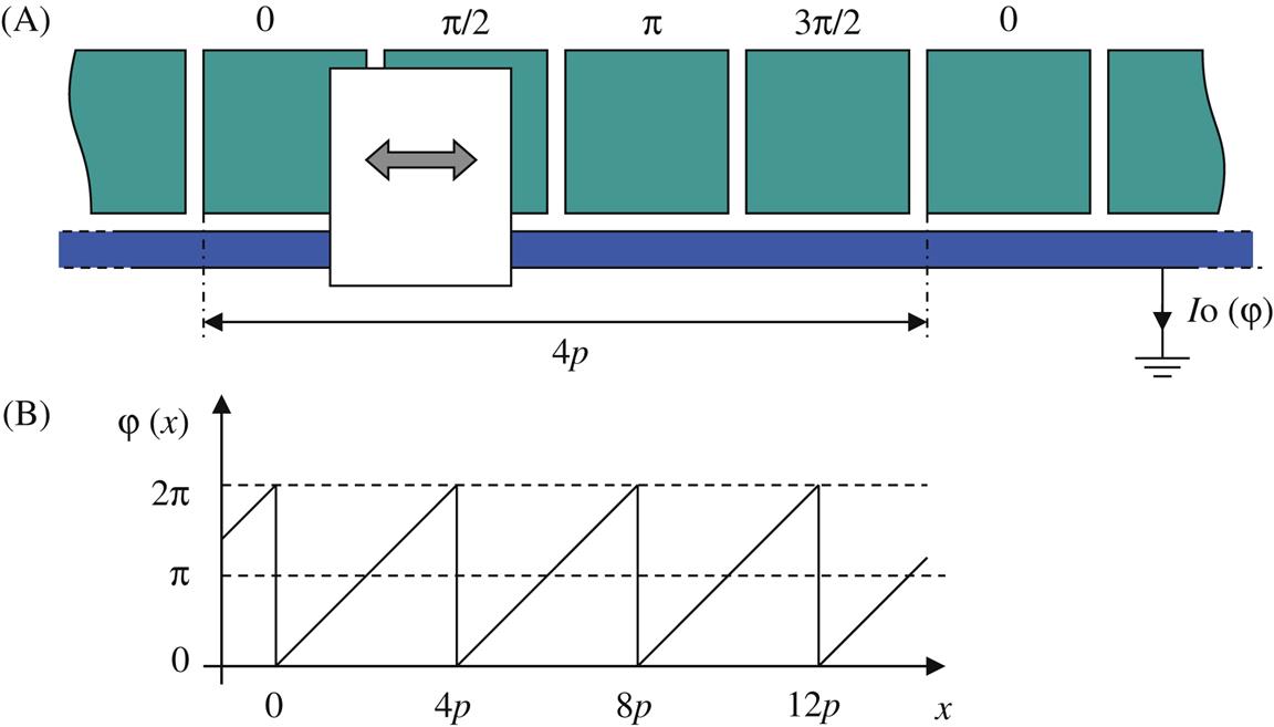
The fixed electrodes in the array are connected to sine wave voltages with phase differences of π/2. When the moving plate travels along four successive sections, the phase of the voltage on this plate changes from 0 to 2π (Fig. 5.9B). This is repeated for each group of four electrodes. Hence the output phase changes periodically with displacement, with a period of four times the plate pitch p. An unambiguous output is obtained by keeping track of the number of passed cycles, using an incremental counter.
The straight lines in Fig. 5.9B are actually four s-shaped curves from Fig. 5.8 in series, but nonlinearity can be compensated for by appropriate shaping of the fixed electrodes. Phase differences can be measured with high resolution, down to 0.1 degree. By periodically repeating the structure, a large range is obtained combined with high resolution. A well-known application is found in some electronic calliper rules: these have a range of about 20 cm and a resolution of 0.01 mm.
Capacitive angular sensors operate in a similar way (Fig. 5.10). The fixed segmented plates are arranged in a circular array and the moving plate is a vane connected to the rotating shaft.

The challenge of the designer is to obtain the highest possible resolution over a fixed range of 2π rad. Various solutions have been proposed, for instance multiple electrodes on the moving part. Evidently, guard electrodes are indispensable here to reduce stray fields. The resolution of capacitive multiplate angular sensors can be as high as 18 bit or 5 s of an arc [9].
5.2.3 Silicon capacitive sensors
Silicon micromachining technology offers the possibility to construct extremely small capacitive sensors. The technology allows the fabrication of very thin membranes, similar to piezoresistive sensors as described in Chapter 4, Resistive sensors. Instead of adding piezoresistors to the spring element, the flexible membrane is opposed to a fixed flat electrode, building a miniaturized flat-plate capacitor. An applied force or pressure difference causes the membrane to deflect, resulting in a capacitance change that can easily be measured. Advances in the technology of MEMS have resulted in the realization of microsensors for other quantities as well, for instance, acceleration. These systems now find widespread applications in automotive and other large volume market segments.
These technologies are highly attractive for accelerometers, rate gyroscopes, and (gas) pressure sensors but less for force sensors because of the susceptibility to mechanical damage of the tiny movable parts. Accelerometers get much attention because the force is introduced simply by the inertia of a seismic mass fabricated on the same chip. Capacitive sensors for other measurands are also considered to be implemented in MEMS technology, for example, the angular sensor is discussed in Ref. [10].
From a technological point of view, however, a capacitive sensor is more difficult to realize compared to its resistive counterpart. The surfaces of the various parts making up a capacitance should be provided with a conducting layer acting as one of the capacitor’s flat plates. Furthermore, the spacing between the plates should be made small, to obtain a reasonable capacitance and sensitivity, and the alignment of the two electrodes is also a critical processing step.
5.2.3.1 Silicon pressure sensors
The first silicon capacitive pressure sensors consist of a stack of three layers: a support layer, a membrane (etched silicon), and a top layer with the fixed counter electrode. The support layer and top layer can be made from silicon or glass. The electronic circuitry resides on the membrane chip or the (silicon) top layer. The layers are connected using special techniques. Fig. 5.11 shows some examples [11–13] of integrated capacitive pressure sensors (vertical scale much larger than horizontal scale). In the configuration in Fig. 5.11B, the electronics and the membrane are made from separate wafers, to enhance technological freedom: the processes for etching membranes and deposition of electronic circuitry are not fully compatible. The figures show only a general layout; details can be found in the cited papers.

A large variety of alternative structures have been proposed over the last decennia. In Ref. [14] the membrane chip is positioned flipped at the top, whereas a reference capacitance is included in the structure. A structure without separate top layer is described in Ref. [15]. Both capacitor plates are constructed on the membrane chip using surface micromachining. The gap is realized by selective etching of a so-called sacrificial layer, positioned between the two electrode layers. Here, too, a reference capacitor (insensitive to pressure) has been integrated.
Due to the small dimensions of the structures (in the order of millimeters), the capacitance value is small too, and the change caused by the measurand is even smaller. A larger (initial) capacitance may be realized by reducing the gap distance between the plates. However, electrostatic (attractive) forces between the plates can easily result in “buckling” and short-circuiting of the capacitor. The alternative is to increase the effective surface area. This can be realized by a supporting dielectric structure, as is applied in Ref. [16]. The sensor is made up of two processed wafers, put together face-to-face and resulting in a narrow gap between them. After bonding the two wafers, the substrate of the top layer is removed by selective etching, leaving a thin membrane (2.5 μm) as the remainder of the top wafer. The membrane is supported by a hexagonal grid of a dielectric material that prevents it from collapsing. In this way a relatively large area combined with a narrow gap is achieved, and hence a larger capacitance and sensitivity can be obtained than with other techniques.
5.2.3.2 Silicon accelerometers
Many accelerometers are based on capacitive sensing techniques, for instance the accelerometer with feedback as introduced in Chapter 3, Uncertainty aspects. A few decennia ago it was shown that the complete system can be integrated on silicon, resulting in a small, easy-to-mount device [17].
Capacitive accelerometers made in MEMS technology are basically structured as given in Fig. 4.23 (a piezoresistive accelerometer): they consist of a seismic mass suspended on flexible beams. Instead of integrated piezoresistors, electrodes are deposited on proper places in the structure forming flat-plate capacitors. The mass moves due to an inertial force, resulting in a change in distance between the plates, and this causes the capacitance to change. By a special configuration with three or four masses and associated electrodes, it is possible to realize a 3D accelerometer in a single piece of silicon [18]. Together with the MEMS sensor, additional electronics, and signal processing, for instance voltage regulators or an ASIC (application-specific integrated circuit) and a temperature sensor for offset compensation can be housed in a small package [19].
Micromachined acceleration sensors suffer from small capacitances too and hence have low sensitivity. A larger (initial) capacitance might be realized by a dielectric support structures (see the preceding section on pressure sensors). Another way is to increase the effective surface area. This is realized in MEMS technology, allowing the construction of so-called comb structures. Fig. 5.12 shows the basic configuration.
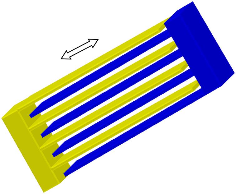
When the two combs move relative to each other in the direction of the arrow, the effective surface area of the capacitor changes. The more fingers, the larger the surface area and the higher the capacitance. Such structures, and even more complicated configurations, can be readily made using advanced MEMS technology. The same structure is also used for capacitive actuators, so-called comb drives.
5.3 Interfacing
5.3.1 Interfacing with analog circuits
In high-resolution sensors and microsensors, the capacitance changes that have to be measured can be extremely small (down to fractions of a femtofarad or 10−15 F). Adequate interfacing is required to preserve the intrinsic performance of the sensor system. We discuss four major analog interface methods for capacitive sensors (Fig. 5.13):
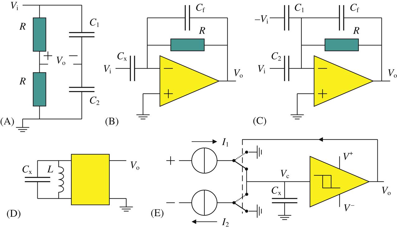
For each of these methods, we give a brief analysis (see Appendix C for the transfer of operational amplifier configurations). The bridge transfer (Fig. 5.13A) is:
(5.16)
In a single sensor configuration, C1=C+ΔC and C2=C, hence
(5.17)
The transfer is frequency independent but nonlinear. In a differential or balanced configuration, C1=C+ΔC and C2=C−ΔC, thus
(5.18)
Clearly, the differential mode yields better linearity and a wider dynamic range (see also Chapter 4, Resistive sensors, on resistance bridges). A proper measurement of the bridge output voltage requires a differential amplifier with high input impedance and high common mode rejection ratio.
Interface circuits based on current–voltage measurements are shown in Fig. 5.13B and C: the first for single mode operation and the second for differential mode operation. If resistance R is disregarded, the transfer function of the single mode circuit is
(5.19)
and for the differential mode:
(5.20)
Again the advantage of a balanced configuration appears immediately from expression (5.20), which is linear, and the output is zero in the initial state (equal capacitances). The transfer is frequency independent if resistance R in Fig. 5.13C is left out. However, the circuit does not work properly in that case (see Appendix C) due to integration of the offset and bias currents of the operational amplifier. The resistance R prevents the circuit from running into overload but causes the transfer to fall off with decreasing frequency from about f=1/2πRCf. This means that the frequency of the interrogating signal Vi should be chosen well above this cut-off frequency.
When the maximum capacitance change is small, the feedback capacitance Cf should be chosen small too, for a reasonable gain of the circuit (as follows from Eq. (5.20)). However, stray capacitances (wiring, input capacitance of the amplifier) set a limit to the minimum value for Cf (to some pF). In integrated capacitive sensors, these stray capacitances are very small, allowing a small feedback capacitance, hence high gain.
The sensitivity is limited by the stability of the initial state (where the output should be zero). Neither the amplitude drift nor the frequency instability of the oscillator affects the zero stability since they are common to both differential sensors. The performance of the measurement is mainly limited by the phase difference between the two AC voltage sources. The output appears to be very sensitive for deviations from the required 180 degrees phase difference, a fact that can be used to create a sensitive capacitance-to-phase converter [20].
A simple though rather inaccurate method for measuring capacitance changes is the conversion to frequency, shown in Fig. 5.13D. The capacitance is part of an LC-oscillator circuit that generates a periodic signal with frequency
(5.21)
where f0 is the frequency in the initial state. An advantage of the oscillator method is easy signal processing with a microprocessor: the frequency can be determined by simply counting the number of clock pulses during one cycle of the oscillator signal. Obviously, the other circuit elements must be stable and the oscillation process should be guaranteed over the entire capacitance range. A detailed analysis of a circuit based on this principle can be found in Ref. [21]. The interface contains a microprocessor-controlled feedback system with a voltage-controlled oscillator, which keeps the actuation frequency equal to the resonance frequency of the LC-circuit. This interface has a sensitivity of 100 Hz/fF and a resolution of about 0.1 fF.
An interface circuit that combines the advantages of a time signal output and high linearity is given in Fig. 5.13E, an example of a relaxation oscillator. The unknown capacitance is periodically charged and discharged with currents I1 and I2. During charging, Vc increases linearly with time until the upper hysteresis level of the Schmitt trigger (Appendix C) is reached. At that moment the switches turn over and the capacitance is discharged until the lower hysteresis level is reached. The result is a periodic triangular output signal with fixed amplitude between the levels of the Schmitt trigger and a frequency related to the capacitance according to:
(5.22)
where Vs is the hysteresis range of the Schmitt trigger. The method yields accurate results because the frequency depends only on these fixed levels and the charge current.
5.3.2 Interfacing to embedded systems
In the previous section the sensing device is always a capacitor of which a particular parameter (A, d, or ε) changes due to a measurand. The alternative of this so-called internal capacitance is the external capacitance, that changes by human presence. In embedded systems a common way to measure capacitance is by measuring the time to charge or discharge this capacitor or capacitive sensor. The use of an RC-network allows the designer to set the order of magnitude of the measured charge time. This enables also a trade-off in implementation between sample time and resolution: a long measurement time allows for a high resolution (many time-steps) but also a low sample rate (caused by the time between measurements). The method is suitable for both external and internal capacitances.
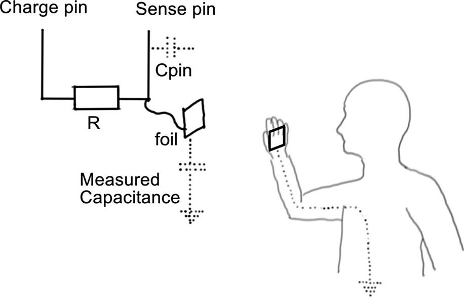
Fig. 5.14 shows a schematic method for measuring externally caused variations in capacitance, using a microcontroller. One side of a capacitor is formed by a piece of conducting material, such as an antenna or section of a foil. One pin of the microcontroller is used to charge this capacitor; the other pin is used as digital input to detect the moment when this charge voltage exceeds a certain level, normally defined by the logic level of the digital input. In a 5 V microcontroller system such as the earlier discussed Arduino, this level lies around 2.5 V. This means that the capacitive sensor is charged until it reaches 2.5 V. After this the capacitive sensor can be fully discharged by making the detection pin an output, simply by short-circuiting the capacitor to completely discharging it. As soon as the capacitive sensor is completely discharged, the cycle can start again. Note that no analog voltage is measured, just the time it takes to fully charge the capacitor formed by the foil and the human presence.
A similar approach can be used for measuring an internal capacitance (Fig. 5.15). The resistance value R has to be chosen in a range such that the charge time can be measured with sufficient resolution by the microcontroller system. Appendix D shows some code examples and lists some libraries facilitating (external) capacitive sensing using an Arduino board.

The described method uses the microcontroller input- and output-pins to charge, discharge, and detect the voltage level of a capacitor. Instead of sensing a change in capacitance, the voltage used to charge the capacitor can be measured using this strategy. With fixed values for the capacitor and resistor, so a fixed value of RC, the charge voltage, will be determined by the input voltage. This approach allows for a simple, albeit nonlinear, analog to digital conversion, which can be implemented using a single microcontroller pin. Since the nonlinearity is highly predictable (it is a first-order RC-network), the relation between measured time and input voltage can be linearized.
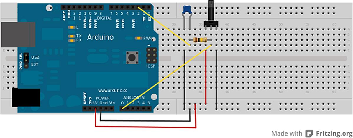
Fig. 5.16 shows an Arduino board with breadboard, an RC-network (100 nF, 100 kΩ), and a potentiometer as analog sensor or voltage source. In this case the voltage is measured simultaneously with one of the analog to digital converter’s input pins and with the RC-network connected to pin 2. By making pin 2 an output, the capacitor can be fully charged (or fully discharged). After switching back to input (high impedance), the capacitor will be discharged (or charged) by the sensor voltage supplied by the potentiometer (acting as a position sensor here). The charge time t depends on V(t), dictated by V(t)=Vsource {1−e−t/RC}, with fixed values for R and C.
This strategy allows turning any regular microcontroller pin into an analog sensing pin; especially when the amount of analog inputs is limited (or unavailable) this approach might be beneficial. Commercially available optical array sensors like the one shown in Fig. 5.17 already have built-in capacitors for this very purpose, taking into account the usually limited availability of analog inputs on conventional microcontroller systems. Although the sensor is in the optical domain, the applied interfacing strategy is capacitive.

5.4 Applications
5.4.1 Capacitive sensors for position- and force-related quantities
Capacitive sensors are suitable for the measurement of all sorts of position-related quantities: displacement, rotation, speed, acceleration, and tilt. Combined with an elastic element, force, pressure, torque, and mass sensors can also be realized using capacitive principles. Most of these sensors are based on Eq. (5.1), indicating the relation between the capacitance value and a geometric parameter (e.g., effective surface area and plate distance). Capacitive sensors are particularly suitable for applications with high demands (for instance extreme temperatures). The mechanical construction is simple and robust. Furthermore, extremely small capacitance changes (down to 1 fF) can be measured with simple interface circuits. Finally, stray capacitances and other capacitances due to wiring and amplifiers can easily be eliminated using guarding, virtual grounding, and proper interfacing.
As with all displacement sensors, capacitive displacement sensors can be modified to make them suitable for the measurement of angular rate, acceleration, force, torque, mass, and pressure. Differential configurations are recommended and, where appropriate, a feedback principle as well, to reduce intrinsic sensor errors (refer to Chapter 3, Uncertainty aspects, for a capacitive accelerometer based on feedback). Table 5.2 resumes some specifications of commercial capacitive sensors for various measurement quantities.
Using the circular multiplate capacitor discussed in Section 5.2.2, angular position and angular speed can be determined with high accuracy, as has been demonstrated in many papers, for instance in Refs [22–24]. With a careful design, angular position sensors can have a resolution of 18 bit, a reproducibility of 17 bit and an absolute accuracy better than 14 bit. A micromachined contact-free angle sensor was already mentioned in Section 5.2.3 [10]: this angle sensor combines an inductive principle for the transduction from angle (with respect to a fixed magnetic field) to the deflection of a polysilicon micromass and the capacitive measurement of this deflection. A planar micromachined gyroscope is described in Ref. [25] with a balanced capacitive read-out circuit. A graphical impression of this micromachined structure as can be found in gyroscopes and accelerometers is shown in Fig. 5.18.

With capacitive sensors, the torque on (rotating) axes can be measured [26–28]. In some of these applications the sensor on the axis is purely passive, which means that no power supply on the axis is needed. The information transfer to and from the axis is accomplished either inductively or with pure capacitive techniques.
The capacitive mass sensor in Ref. [29] uses a metal spring as the elastic element; this sensor is designed for a low-temperature sensitivity, for which thermally stable materials have been selected. The capacitive force sensor in Ref. [30] contains an elastic dielectric; its basic configuration is depicted in Fig. 5.19.
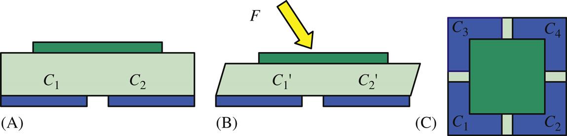
It is sensitive in two shear directions and the normal direction. At zero force, all four capacitances C1−C4 are equal. A pure normal force will increase each capacitance equally, and a pure shear force results in an increased difference between adjacent capacitances (differential method), according to the direction of the applied shear force. The interface should be able to distinguish between these force components.
5.4.2 Sensing applications using internal capacitances
In this section examples of capacitive measurements for a variety of applications are discussed, illustrating the versatility of the capacitive sensing method. Selected measurands are distance, displacement, thickness, rotation, strain, force, level, and flow. Some special applications concern the detection of persons and rain on a car’s windscreen.
Capacitive sensors offer the possibility of highly accurate distance or displacement measurements, as in controlled x–y tables. A capacitive sensor designed for product inspection is given in Ref. [31]. The goal is to measure the inner diameter of cylinders using a co-ordinate measuring machine with touch probe. In this work the bending of the touch probe (a thin stylus) is determined by capacitive means. The method allows measuring of internal diameters less than 0.3 mm, with an accuracy of 1 µm.
Coating thickness can be measured in several ways. For a nonconductive coating on a conductive plate, the capacitive method is suitable to measure the thickness of such a coating. An example of this method is given in Ref. [32], proposing a capacitive probe and giving an analysis of the various sources of errors.
In Section 5.2.2 multiple plate capacitive sensors were discussed, to enlarge the range of a (linear) displacement sensor. An alternative solution is given in Ref. [33], where a configuration is presented similar to the inductosyn given in Chapter 6 on inductive sensors. The sensor consists of two printed circuit boards (PCBs), each provided with an array of electrodes (transmitter and receiver), able to slide linearly over each other as in an optical encoder. The signal transfer from transmitter to receiver is determined by the configuration of the electrodes and shows a triangular course with displacement. Although realized with simple technology (e.g., PCBs, copper electrodes, and coating), the resolution of the sensor appears to be about 126 nm, over a range of 20 mm.
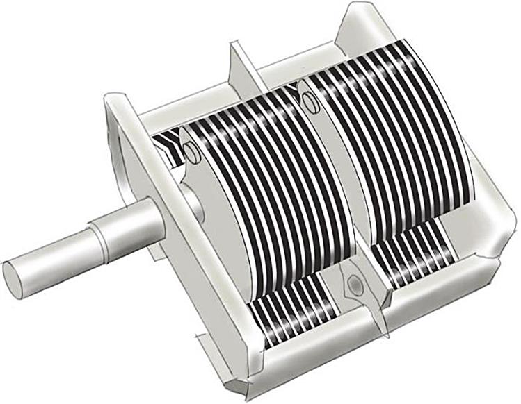
Not only linear displacement but also rotation can be measured accurately by capacitive means. The classical example is the “trimmer” or rotary capacitor, which uses a series of parallel plates with overlapping region A. Rotating one set of the plates will change the total active surface area of the capacitor, shown in Fig. 5.20. An example with segmented electrodes was given in Fig. 5.10. A modified version is presented in Ref. [34], having a completely isolated rotor. The main advantage of this design is that no electrical connections to the rotating part are needed.
A totally different application of a capacitive sensor is found in Ref. [35]: the measurement of tire strain. Car tyres are usually reinforced with layers of steel wires. When the tire is loaded, the resulting strain causes the distance between these wires to increase. Hence, the capacitance between the wires changes accordingly. The paper describes how to measure this capacitance change. The interface is based on an oscillator (like in Fig. 5.13D), but instead of an LC-oscillator, an RC-oscillator is chosen. Wireless read-out allows strain measurement during rotation of the wheel with tire. Another approach to measure tire strain using a capacitive method is described in Ref. [36]. The authors have fabricated a particular strain gauge, consisting of a pair of interdigitated flat electrodes on a flexible polyimide carrier. The gauge, glued onto the inside tire, responds to strain by a change in capacitance [37].
As mentioned before, capacitive sensors can also be applied for force and pressure measurements. A particular application is on-line weighing of (for instance) cars [38]. The sensor consists of two rubber layers sandwiched between (three) conductive sheets. When pressed, the distance between the conductive sheets becomes smaller, producing an increase in capacitance. The sensor is flexible, light-weight, and easy to carry. It can simply be positioned on the road and is capable of dynamically measuring the weight of a (slowly) passing car.
Thus far we have used the geometric factor G in Eq. (5.5) as the basis for a capacitive measurement. The dielectric constant εr is another parameter determining the capacitance value of a capacitive structure and hence a workable method for sensing. Measuring liquid level in a tank is an obvious example. A pair of flat-plate electrodes hanging vertically in a tank represents a capacitance that depends on the dielectric constant of the fluid between these plates (Fig. 5.21A).

In an empty tank this is air (or another gas with εr≈1), in a full tank the liquid (for instance water with εr≈80). A partly filled capacitor can be conceived as two capacitors in parallel: one filled with the liquid up to the upper level (CL), and one with air from the level to the top of the plates (CA). The total capacitance is the sum of these two capacitances, and hence a measure for the level. Obviously, this method holds only for nonconducting liquids. Since water is both dielectric and conductive, at least one of the electrodes should be isolated from the liquid, and special measures have to be taken when the container is grounded, which is explained in Ref. [39]. By inserting two reference capacitors, one at the top (in air) and another at the bottom (in the liquid), as shown in Fig. 5.21B, the influence of several parameter variations can be eliminated [40]. Instead of one continuous capacitor, an array of smaller capacitors Ci can be conceived, resulting in a discrete output (Fig. 5.21C). In Ref. [41] such a solution is presented, with a resolution of 0.1 mm in level. Furthermore, Ref. [42] shows how a capacitive sensor structure can be used to detect unbalanced load in a washing machine.
The capacitive method makes it possible to detect water drops on a windscreen: a rain sensor. It consists basically of a pair of flat coplanar electrodes; the dielectric is composed of three parts: at the back side glass, at the front side air and/or water. To be less sensitive to temperature variations and other possible common mode interferences, a differential structure is preferred: one capacitor is exposed to water, the other is not and serves as a reference capacitor [43].
The dielectric constant of a human being differs substantially from that of air, which makes it possible to capacitively detect the presence or passage of persons. Pavlov et al. [44] describe a configuration with small electrodes located in a doorway, giving a capacitance change of a few tenths pF when a person passes. The interface is based on the oscillation method and with special signal processing it is also possible to extract particular features of the passing person, for instance high or low speed and direction. George et al. [45] discuss a capacitive method to detect the presence of a person on a car seat. The seat is provided with a set of electrodes in the seat as well as the back rest. The sensor configuration enables the discrimination between an adult and a child, and between persons and objects (for instance bottles with water). Another capacitive technique for occupancy detection is presented in Ref. [46]. The method is based on an impedance model of biological tissue, being part of the dielectric between two electrodes in the seat. The measured impedance parameters are compared with the model parameters, from which information about the occupancy is derived. An extension to position of humans is presented in Ref. [47]; large flat electrodes are integrated in the floor and walls of a 2×2 m room. A detailed analysis of the changes in the various capacitors building up this configuration shows that it is possible to locate persons with reasonable resolution. This approach of human presence sensing differs from the approach that will be described in Section 5.4.3 where external variation in capacitance is measured, caused by human presence. In that situation the human is actively forming part of the capacitor—or a parallel capacitance to the existing one.
One of the many ways to measure flow velocity of a substance moving through a pipe is correlation: two sensors placed a distance d apart from each other measure some property of the flowing substance, for instance reflection (scattering), acoustic noise or thermally induced temperature variations. The cross correlation of the (noisy) signals is maximal for a delay time equal to τ=d/v from which the velocity is determined. An implementation using a capacitive principle is found in Ref. [48], applied for a flow of granular solid. Two ring-shaped electrodes are mounted at the outside of the pipe, a distance d apart and a third electrode just midway between them. Due to the nonhomogeneity of the flowing material, the capacitances of these two capacitors show random fluctuations. The flow velocity is found from the cross correlation of the two capacitance signals.
A magnetic flux can also be measured using a capacitive principle [49]. A varying magnetic flux in a (ferromagnetic) material produces eddy currents (see Chapter 6), which in turn create a voltage difference across the material. This voltage can be measured using, for instance, the needle method: two needle-like probes are pressed on the surface of the material under test, and the potential difference is a measure for the eddy currents and hence the magnetic flux. To be able to measure in this way, the needles must make electrical contact, so any possible isolating coating should be removed at the contact places. In Ref. [49] the needles are replaced by conductive pads acting as pick-up electrodes: the voltage is coupled capacitively to the measurement instrument. Calculations show that the voltages are small (mV range) but measurable, if precautions are taken as outlined in the previous sections: differential configuration, guarding, and proper filtering.
A common application of a capacitive sensor in consumer products is the condenser or electret microphone. This microphone functions as an electrostatically charged device, using permanently charged material. Commercially available electret microphones need a simple circuit consisting of a resistor to supply a bias voltage, together with a capacitor for decoupling any DC offset (see Fig. 5.22). By changing the distance between two charged plates, one being stationary, one being the diaphragm that is moved trough air pressure, the capacitance of the sensor changes. This change can be measured and amplified. Although size and characteristics might vary, the main application for these microphones lies in the audio domain, that is, 50–20,000 Hz.

This section clearly shows that the capacitive sensing principle can be applied in numerous situations. The configuration is simple, a balanced mode is preferred, and proper interfacing may reduce the influence of stray and cable capacitances on the sensitivity and stability of the transfer.
5.4.3 Sensing applications using external capacitances
By changing internal parameters such as plate size (overlapping surface area), inner-plate distance, and dielectric properties, the capacitance value of the capacitor changes, turning the capacitor into a sensor. Besides this “internal” sensing, as discussed in Section 5.4.2, a capacitor can also be used as a sensor for external variations in capacitance, caused by the presence of other objects. Instead of the presence of external objects, also human presence, that is, the position of hands or fingertips, can be measured. This section discusses some examples of external sensing.
The classical example of a device sensing external variations in capacitance is the Theremin organ. Invented and patented in 1928 by the Russian inventor Léon Theremin [50], this device is also among the first electronic instruments ever designed. By changing the position of the player’s hands with respect to two antennae, volume and pitch of the generated tone are changed. The antennae form part of capacitors in LC-oscillator circuits. By changing the capacitance C, the frequency of the oscillator changes, according to Fig. 5.13D. Fig. 5.23 shows a modern design of the classic instrument.

The fact that, using capacitive sensors, the proximity of fingers or a hand can be detected without making electrical contact makes it an ideal technology for measuring human input. For example in situations where input (i.e., pressing a button) is necessary in an environment that is wet, or needs to be sterile, capacitive touch sensors can provide a solution.
The antenna shown in Fig. 5.23 can detect proximity of a human hand—the instrument, however, requires frequent calibration. The amount of charge, ground contact, and capacitance of the player may change over time, even during play.
By designing patterns whose capacitance change by imposing human presence, this negative side effect can be omitted. A nice example is the capacitive “click wheel” that has been used as rotational input device on audio players, shown in Fig. 5.24. This wheel consists of a number of foil segments, the capacitance of each is sensed with respect to the others.

The principle of a simple linear slider is shown in Fig. 5.25. By taking the difference between two segments and comparing that number with the total measured capacitance, a reliable indication of the finger position can be given. The position is relative to this change, that is, (A−B)/(A+B).

A capacitive touch-sensor can be manufactured using a grid of conductive strips, manufactured transparently in glass. This sensor can be placed on top of an LCD display, thus forming a touchscreen that is widely used for human input in devices such as smartphones. A schematic overview of such a touchscreen is given in Fig. 5.26. This array of small capacitors is influenced by the presence of human fingers, and, contrary to the resistive touchscreen described in the previous chapter, can detect presence of multiple fingertips at the same time. The signal processing that is needed to determine the position of the fingertips bears similarities with image processing. It requires techniques such as thresholding, dilation, and blob-tracking to accurately measure and follow the motion of (multiple) fingertips. A discussion of those techniques is beyond the scope of this book.
