Chapter 2
Alignment, Pointing, and Sizing Instruments

One of the specific properties of laser sources is the ability to supply a well-collimated light beam. In free propagation, the beam of a common laser like the He-Ne laser (see Appendix A1) can be visualized at a distance much larger than an ordinary flashlight can attain. This is a consequence of the low angular divergence of the laser beam and has the well-known application to laser pointers.

The divergence of the laser beam is usually the small value dictated by the diffraction limit. The diffraction limit is reached because the source generates light in the single-mode spatial regime, which is a condition easy to meet, especially with He-Ne lasers. The property of the laser emitting a particularly collimated, directional beam gives instruments used for alignment an advantage, as an extension of the plumb line on a generic direction, which is not necessarily vertical.

Alignment is used for positioning objects along a desired direction, as indicated by the propagation direction of the laser beam. Applications range from construction work and laying pipelines to checking terrain planarity in agriculture. In this last application, the concept is extended by making a laser level that uses a rotating fan beam and defines the reference plane for alignment. Another class of instruments exploiting the good spatial quality of the laser beam, as obtained by single transverse-mode operation, is dimensional measurement by diffraction. The object under measurement is positioned in the beam waist of the laser beam so that the wave front of illumination is plane. Light scattered by the object has a far-field diffracted profile precisely related to the dimensions of the object, so the measurement of it can be developed by analyzing the signal collected by a detector scanning the far-field distribution. Examples of noncontact measurement discussed later in this chapter are wire diameter and fine-particle sizing.

2.1 Alignment

In an alignment instrument, we want to project the beam at a distance of interest and be able to keep its size the smallest possible along the longest possible path.

Because a single-transversal TEM₀₀ mode is the distribution with the least diffraction in propagation, the He-Ne laser has traditionally been the preferred source. The He-Ne laser readily operates in single-transversal mode regime and has a wavelength λ=633 nm in the visible.

Semiconductor lasers may be used as well if the elliptical near-field spot is properly corrected by an anamorphic objective lens circularizing the output beam.

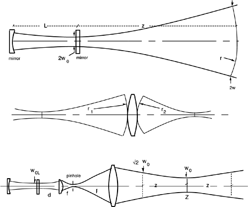
Let us consider the propagation of the Gaussian beam emitted by the laser (see Appendix A1.1), as in Fig.2-1.

The Gaussian beam keeps its distribution unaltered in free propagation and in imaging through lenses, and the spot-size w is the parameter that describes it.

In free propagation (Fig.2-1, top) w evolves with the distance z from the beam waist w₀ as:

(2.1)

In optical conjugation through a lens, the spot size is multiplied by the magnification factor m=r₁/r₂, with r₁ and r₂ being the radii of curvature of the wave fronts at the lens surfaces. The radii obey a formula similar to Newton’s lens formula 1/p+1/q=1/f, that is:

(2.2)

On its turn, the radius of curvature of the wave front, as a function of the distance z from the beam waist, is given by:

(2.3)

From Eq.2.3, we have r=∞ for z=0 (at the beam waist), and r= z for z>>πw₀²/λ (in the far field, where the Newton formula holds).

Fig. 2-1 Alignment using the Gaussian beam of a laser. Top: free propagation out of the laser; middle: conjugation through a lens; bottom: projection of the beam through a collimating telescope.

Now, we may look for the optimum waist w₀ that minimizes the spot size w on a given span of distance, let’s say between –z and +z. To do that, we find the minimum of w² in Eq.2.1 by differentiating respect to w₀² and equating to zero. We thus obtain:

whence the optimum value of beam waist to be projected at a distance Z from the laser is:

(2.4)

By comparing Eq.2.4 and Eq.A1.5, it turns out that the beam waist minimizing the size of the beam on the desired distance –z ..+z is the same of a laser oscillating on mirrors placed at a distance 2z apart.

In the span –z ..+z, the beam size is minimum at the midpoint, w=w₀, and, from Eq.2.1, it becomes at the ends of the span. To be able to project a beam waist w₀ at distance Z from the laser, a collimating telescope is used (Fig.2.1 bottom). The telescope works better than a single lens and can easily adjust the distance Z by small focusing of its ocular. The magnification m=w₀/w_0L is easily calculated as m=(f/d)(Z/F)=Z/Md where M is the magnification of the telescope.

Example. For a laser with a plano-concave cavity and L=20 cm, K=5, we get from Eq.A1.5 w_0L=0.282 mm as the laser beam waist. The location of the waist is just at the output mirror.

If we want to cover a span of z=±20m, then Eq.2.4 gives w₀=2 mm as the necessary beam waist. Then we need a magnification of m=w₀/w_0L=7.1. Taking Z=z=20m and d=10cm, the collimating telescope shall have a magnification M=F/f=Z/md=20/7.1×0.1=28.

In Fig.2-1 bottom, the pinhole in the telescope filters out spots extraneous to the laser mode, for example, originated by the reflection at the second surface of the laser output mirror. This mirror flat is slightly wedged to prevent the second surface from contributing to reflection into the cavity.

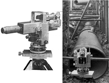
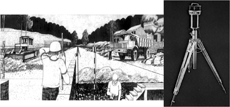
An alignment instrument usually includes a 0.5-2-mW He-Ne laser and a 50-mm diameter telescope providing a magnification of 20-30. The collimating telescope carries a view-finder for target checking. The assembly is mounted on a tripod (see Fig.2-2) and is used for a number of applications in construction work with checks by sight.

Fig. 2-2 A typical alignment instrument, based on a low-power He-Ne laser and collimating telescope, and the application to construction of pipelines. This unit was introduced in 1978 by LaserLicht AG, Munchen.

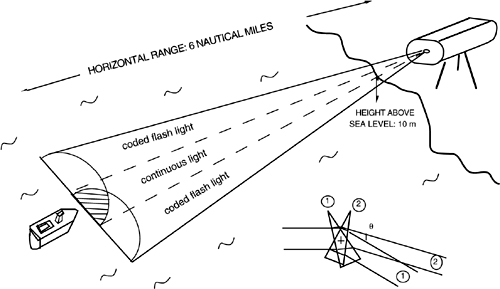
Nearly the same instrument (see Fig.2-3) has been used in harbors to establish a marine channel light that helps boats in their approach to maneuver to the harbor and to avoid dangerous sand bars.

In this application, the beam is switched periodically by a small angle in a horizontal plane through a prism inserted in the beam path. This arrangement provides an error signal that helps the boat to keep the correct homing direction.

Using a He-Ne laser emitting approximately 10 mW in the red (633 nm) and a 10-cm diameter telescope, the beam can be seen by eye at a distance of several miles. The actual range is limited primarily by weather conditions, which affect atmospheric attenuation and turbulence (see App.A3). Of course, in presence of haze and fog, the optical power is attenuated and the useful range drops to about a few times the visibility L_vis (see Eq.A3-4).

Another problem with the marine channel light is laser safety (see Appendix A1.5). To ensure safe view of the laser beam, power density is designed to be less than the Maximum Permissible Exposure (MPE) from a minimum distance onward. If personnel aboard the ship stare at the beam through binoculars, the power density increases by one or two orders of magnitude and ocular hazard may occur.

Fig. 2-3 Alignment instrument used as a marine channel light to help ships maneuver by homing to the harbor. The beam is switched by an angle θ by a prism rotating at approximately 3Hz and is transmitted by a telescope above the sea surface to the ship. In the region of superposition, light appears steady, whereas outside it flashes. Coding semiperiod duration allows discriminating between left and right beams.

2.2 Pointing and Tracking

Centering of the laser spot can be performed by sight, as in construction applications where we just need a resolution of a fraction of the beam spot size, or approximately 1 mm.

For more exacting applications, we may use a photodetector to generate an error signal proportional to the alignment error. The photodetector may either be a special type designed for position sensing or pointing purposes or may be a normal one acting in combination to a reticle or mask, which establishes a spatial reference for the photodetector.

2.2.1 The Quadrant Photodiode

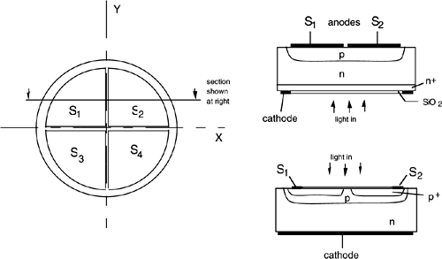
This device has the usual structure of a normal photodiode (see Ref.[1], Sect.5.2), but one of the access electrodes, for example, the anode in a pn or pin junction, is sectioned in four sectors (Fig.2-4, left). Light input is from the chip backside when sections are defined by metallization, and from the top when a p⁺ layers with side-ring contact is used (Fig.2-4, right). Size of the quadrant photodiode may go from 0.2 to 2 mm in diameter. The gap between sectors may be as small as 5-10 μm.

Light impinging on a certain sector originates a photocurrent collected by the correspondent electrode. Thus, we have four signals, S₁, S₂, S₃, and S₄, out of the four-quadrant photodiode.

Fig.2-4 A quadrant photodiode for pointing applications. Left: the segmented electrodes structure; right: section of the pn photodiode structure with metal electrodes for backside light input (top) and section of a p⁺pn structure for front light input (bottom).

We can compute two coordinate signals S_X and S_Y as:

(2.5)

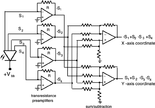
A practical circuit that interfaces the four-quadrant photodiode and computes the S_X and S_Y signals is shown in Fig.2-5. Based on operational amplifiers, the circuit terminates the four anodes of the photodiode on the virtual ground of transresistance preamplifiers ([1], Sect.5.3), that is, on a low-impedance value useful for enhancing the high-frequency performance. The common cathode is fed by the positive voltage (+V_bb) to reverse-bias the photodiodes. Each transresistance stage converts the photodetected current I_ph in a voltage signal V_u=-RI_ph, where R is the feedback resistance of the op-amp. With the four voltages available, it is easy to carry out the sum and difference operation (Eq.2.5) with the op-amps arranged as shown in the second stage.

Fig.2-5 Op-amp circuit for computing the coordinate signals S_X and S_Y from the outputs of the four-quadrant photodiode.

To analyze the dependence of signals S_X (or S_Y) from the coordinate X (or Y), let us suppose that a probe spot scans the photodiode along a line parallel to the X axis. The spot will be smaller than the photodiode usually, but finite in size. Let X represent the coordinate of the spot center, and let R_ph, R_s be the photodiode and spot radii, while w_dz is the dead-zone width.

In Fig.2-6 the coordinate signal S_X is plotted versus X. When X is outside the photodiode by more than the spot radius, the signal is zero. When X is well inside the photodiode, the signal attains its maximum value. When X approaches zero, the signal decreases and reverses its sign, as indicated by Eq.2.5.

Fig.2-6 Dependence of the coordinate signal S_X (or S_Y) from the true coordinate X (or Y) of a light spot falling on the device. When the spot size R_s is very small (R_s/ R_ph=0.01 or less), the response is a square wave with a small dead band near X=0 (or Y=0). When R_s is not so small, the response is smoothed, and we find an almost linear response close to X=0 (or Y=0). The width of the linear region is ±R_s. The dead-zone width w_dz only affects the response for a very small R_s/R_ph ratio.

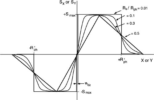
Thus, the response around the X=0 is nearly linear (as shown in Fig.2-6), and the width of linear regime, before S_X reaches saturation, is about ±R_s.

In tracking applications, the outputs from the position sensor are used as the error signals to control the system motion. In this case, the dependence shown in Fig.2-6 is just the desired one to get a good control action, both in acquisition and regulation regions:

- in the regulation region (near X=0), we need a corrective action proportional to the error so that the equilibrium point near X=0 is kept smoothly (without ripple).

- in the acquisition region (large X), the signal shall saturate so that the tracker is driven toward X=0 at the maximum speed.

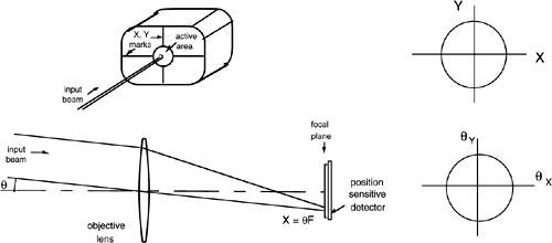
The quadrant photodiode and other position-sensitive devices can be used as a position sensor that measure the X and Y coordinates of the impinging light spot. In this case, we will mount the quadrant photodiode on a positioning stage with reference marks to set the X=0 and Y=0 position (Fig.2-7). The accuracy (σ_X or σ_y) of the coordinate measurement depends on several parameters, such as optical power in the spot, spot shape and its fluctuations, and photodiode dimensions like R_ph and w_dz.

In a well-designed device, typical values are in the range σ_X=0.03 to 0.1 R_ph.

The quadrant photodiode becomes an angle sensor when we place it in the focal plane of an objective lens (Fig.2-7). It measures the angular coordinates θ_x and θ_y of the spot presented in its field of view. Because of the optical conjugation, the coordinates θ_x and θ_y are tied to the spatial coordinate by X=θ_xF and Y=θ_yF, where F is the focal length of the objective lens. The accuracy of the angle measurement follows as σ_θ=σ_X/F.

Fig.2-7 A position-sensing photodiode (either four-quadrant or reticle) can be used as an X-Y coordinate detector (top) or, when it is placed in the focal plane of an objective lens, as an angle-coordinate detector (bottom). In this case, the field of view is θ=R_ph/F.

2.2.2 The Position Sensing Detector

The Position Sensing Detector, or PSD, is a multi-electrode photodiode similar to the four-quadrant photodiode. Developed in recent years as an evolution of the four-quadrant concept, the PSD offers a much better linearity over the entire active area and a response curve independent from the spot size and shape.

Actually, there are mono- and bidimensional PSDs for sensing one or two coordinates. In the following, we describe the bidimensional or array PSD only, because the mono-dimensional or linear PSD follows as a simpler case of the bidimensional.

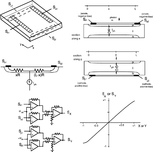
The basic structure of a PSD (see Fig.2-8) is that of a normal pin junction with thin p and n regions. The electrodes for the X and Y coordinates are metal stripes deposited on opposite faces of the chip. Electrically, the stripes are like the normal anode and cathode of a photodiode, yet they are placed at the edges of the p and n regions and sectioned. The doping level of p and n regions is kept much lower than in a normal photodiode to enhance the series resistance of the undepleted p and n regions facing the junction, contrary to what is common.

Fig.2-8 Structure of the PSD photodiode is a normal pin junction, with thin p and n regions, lightly doped or implanted. Light impinging at the point x,y generates a photocurrent that is shared between the X and Y electrodes. Coordinate signals are obtained as the difference between the currents exiting from the electrodes, S_x2-S_x1 and S_y2-S_y1. To ensure good linearity and to have a negligible dependence from R, the currents are sunk by the virtual ground of a transresistance stage. The non inverting inputs of the op-amp stage are used to set the bias, +V_bb and -V_bb, of the X and Y stripes.

The typical resistance R between the stripe contacts (S_x2 and S_x1) is about 10-100 kΩ.

Following the absorption of photons at point x,y (Fig.2-8), photogenerated electrons and holes are swept away quickly by the electric field at the junction. Thus, the current I_ph to be collected reaches the undepleted p and n regions without appreciable error in transversal (x,y) position.

The hole current arrives at point x in the p region (Fig.2-8, top) and shall cross series resistances xR and (L-x)R before reaching the electrodes S_x1 and S_x2. The electron current has a similar response with respect to the electrodes S_y1 and S_y2, but has formally the opposite sign (-I_ph) as it conventionally enters the electrodes.

Because of the series resistance, the current I_ph is shared by the electrodes proportional to the divider ratio of the respective conductances (xR)^-1 and (L-x)^-1R^-1. Therefore, the currents from S_x1 and S_x2 are:

(2.6)

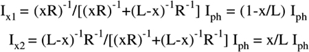
Similarly, the current -I_ph arriving in the n region is shared by the S_y1 and S_y2 electrodes, and Eq.2.6 holds with y in place of x and -I_ph in place of I_ph:

(2.6’)

To recover the currents without errors induced by a finite load resistance, the best approach is to terminate the photodiode outputs (S_y1, etc.) on the virtual ground of op-amps, as shown in Fig.2-8. With this scheme, we get a very low-resistance termination, and the current I_x is deviated in the feedback resistance where it develops an output voltage –R’I_x.

In addition, the use of the op-amp allows an easy biasing of the PSD electrodes. Because of the virtual ground, the inverting input voltage is dynamically locked to that of the noninverting input, and here we will apply the appropriate bias, positive (+V_bb) at the cathode and negative (-V_bb) at the anode. The best for V_bb is half the value of the supply voltage (+V_BB and -V_BB) feeding to the op-amps.

With op-amps, it is easy to compute the coordinate signals S_X and S_Y as the differences of the transresistance-stage outputs (Fig.2-8, bottom left):

(2.7)

Even better, if we add a voltage-controlled gain stage (not shown in Fig.2.8), we can divide outputs S_X and S_Y by I_ph and obtain coordinate signals independent from the impinging optical power P= I_ph/σ (or PSD spectral sensitivity σ).

Often, instead of a fine spot we may have an extended source as the optical input to the PSD. In this case, the coordinates supplied by the PSD are the center of mass of the extended source. This can be easily seen by considering that the power p(x) between x and x+dx, which gives a contribution xp(x) to current , equal to the mean value of p(x).

Commercially available PSDs have a square active area with 0.5-5mm side and are mostly in silicon for a spectral response from 400 to 1100 nm.

Linearity error is less than 0.5% within the 80% of the active area, and cross-talk of coordinate signal is usually less than 10^-4. Response time is usually limited by the large junction capacitance, C_b≈1-50 pF, and by the op-amp frequency response. With 100-MHz op-amps, the response time of coordinate signals may go down to 3-10 μs.

2.2.3 Position Sensing with Reticles

Sometimes, we may not be able to use four-quadrant or PSD photodiodes and may merely have available a normal single-point detector. Nevertheless, we can realize a position-sensing or angular-sensing sensor by placing the detector behind a rotating reticle. Reticles have been developed and used since the early times of thermal-infrared technique [2] to track hot spots with a single-point detector.

In its simplest form, the reticle is a half-transparent and half-opaque disk, as illustrated in Fig.2-9. When put into rotation, it actually works as a chopper of the radiation reaching the photodiode located in the focal plane.

Fig.2-9 Position sensing by a rotating reticle. Light from a bright spot at the angle θ is imaged by the objective lens on the focal plane, where it is chopped by the reticle placed in front of the photodetector. By comparing the phase shift of the square waveform from the photodetector and of a reference, the position Ψ₀ of the source is determined. The amplitude of the signal carries information on the polar coordinate ρ similar to Fig.2-6.

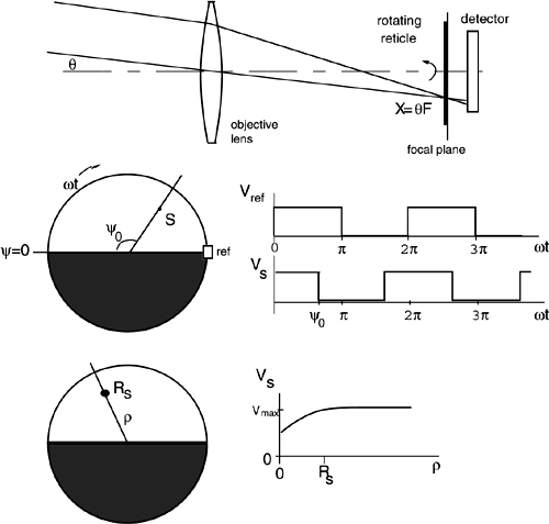
Thus, if we have a single bright spot in the field of view, the photodiode current will be modulated into a square wave, as shown in Fig.2-9. The information about the angular coordinate Ψ₀ of the source is contained in the phase shift of the signal waveform with respect to a reference square wave at Ψ₀=0.

It is easy to get this reference square wave, for example, by a microswitch or with a Light Emitting Diode (LED)-and-photodiode combination placed on the edge of the reticle, as shown in Fig.2-9. The radial coordinate ρ can also be determined by looking at the amplitude V_s of the square wave. With the same argument leading to the dependence plotted in Fig.2-6, we have the diagram of V_s versus ρ reported at the bottom of Fig.2-9.

The plain black/white reticle works well with point-like sources, but is disturbed by the presence of extraneous extended sources in the field of view.

Rejection to extended sources is improved by the rising sun reticle (Fig.2-10, top). In this reticle, half of the circle has 50% transmission, and half has 0 or 100%-transmission sectors, averaging 50% on the entire reticle. As a result, a point source gives a response with large amplitude V_s, whereas details larger than the sector width have V_s≈0 and only add a continuous component to the output signal.

Fig.2-10 The rising-sun reticle provides an improved suppression to extended sources (top). The digital readout reticle (bottom) supplies both ρ and Ψ coordinates in digital format.

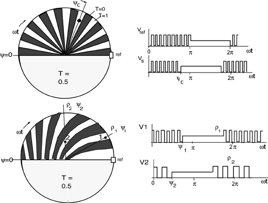
The readout of the angle coordinate Ψ can be made digital by counting the periods elapsed between the signal down-going edge (electrical angle Ψ₀) and the reference down-going edge (electrical angle π). See the waveforms in Fig.2-10.

Another interesting reticle allowing an all-digital readout of coordinates is the digitizing–sector reticle shown in Fig.2-10, bottom. Here, the sectors are shaped according to a special radial profile. We choose the profile so that a point source at a radius ρ intersects a number of sectors proportional to ρ.

Thus, by counting the number of periods contained in a complete 2π-rotation of the reticle, we get the digits of the radial coordinate. The angular coordinate Ψ is determined, as before, by the delay between the downgoing edges of signal and reference and is digitized when the delay is sorted out by period counting. As an example, in Fig.2-10, the signal for point 1 has 7 periods in a half turn while the signal for point 2 has 4 because its radius is smaller. The angular coordinate Ψ₂> Ψ₁ is seen to correspond to a different number of periods between Ψ and π.

For sake of clarity, reticles in Fig.2-10 have been shown with a small number of sectors. In a real reticle, we want to increase the number of sectors as much as possible to improve resolution and dynamic range of the readout.

The limits are set by the smallest detail we can write into the optical layer of the reticle, usually a metal film on a glass substrate. Using photolithographic techniques, we can easily attain a few-μm detail on a few cm-side reticle, or a 10^-3 to 10^-4 relative resolution or potential number of sectors. This argument explains how a 10-bit resolution in the digital readout of ρ,Ψ coordinates is achieved with rotating reticles.

2.3 Laser Level

The laser level is an extension of the concept of point-like alignment described in Section 2.1. When we do not need a direction to follow, or two coordinates (spatial x,y or angular ρ,Ψ) as exemplified by the pipeline alignment, but rather a single coordinate (the height z or the horizontal φ) with the others free, the laser level is the instrument we need.

The most common application of the laser level is the distribution of the horizontal plane in construction works (Fig.2-11) and in leveling (or slope removing) of cultivation terrain subject to intensive watering, like rice. In this case, leveling is very important to save huge quantities of water.

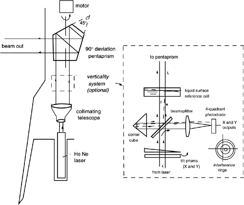
As shown in Fig.2-11, a laser level can be implemented by a tripod-mounted laser. The laser source carries a collimating telescope to minimize the spot size on the range to be covered, as explained in Section 2.1. In addition, we transform the beam in the desired fan shape. This may be accomplished by reflecting the beam with a rotating mirror, oriented at 45 degrees to the vertical (Fig.2-12).

To generate a horizontal plane, the mirror is carefully oriented at 45 degree, and the beam from the laser is oriented vertically. Errors from the nominal angles result in a tilt error of the fan-beam plane.

Fig. 2-11 Alignment with a laser level. Left: use of the level for height relief in construction works. A fan beam is distributed down a 20-50 m radius area, and its position is checked at sight with the graduated stick. Right: a typical tripod-mounted, laser-level instrument developed by Spectra Physics.

The mirror angle-error can be eliminated by using a pentaprism in place of the mirror. The pentaprism has a dihedral angle of 45 degrees and therefore steers the input beam of 90 degrees, irrespective of the angle of incidence (Section A2.2).

Now, we have to adjust the laser beam to the vertical. A spirit level may be used for low cost. For maximum simplicity, the spirit level can be incorporated in one tripod leg, but in doing so, the resolution is modest (≈10mrad or 30arc-min).

Otherwise, we may provide the instrument with a mechanical reference plane perpendicular to the laser beam, and the user will adjust the legs to verticality using a spirit level sliding on this reference plane.

For a good resolution, however, we may need a relatively bulky spirit level (50-cm side for ≈1mrad). Alternatively, we may use an optical method to check the verticality of the laser beam. One method to do so is comparing the beam wave vector to the perpendicular of a liquid surface.

As illustrated in Fig.2-12, the liquid (water) is kept in a hermetic box, and we use a small reflection (≈3%) of the main laser beam passing through it toward the output. The other glass surfaces of the bow are antireflection coated.

Another small (≈3%) portion of the laser beam is picked at the beamsplitter (Fig.2-12 right), which is also antireflection coated at the second surface.

The two beams are recombined by the beamsplitter and come to an objective lens acting as the input of an angle-sensing detector (Fig.2-7). An angular error of verticality produces a tilt in the wave vector reflected by the liquid surface, and then the two beams come to the focal plane of the objective with different directions. Thus, they will produce interference rings in an offset position with respect to the optical axis of the angle-sensing detector (Fig.2-12, bottom right). The detector supplies the coordinate signals θ_X and θ_Y of the center of the interference figure. These signals can be used directly, displaying them to the user, for a manual adjustment of the legs of the tripod, or, with added sophistication, they may be fed to actuators moving a pair of deflecting prisms to adjust the beam and dynamically lock its direction to the vertical.

Fig. 2-12 A laser level uses a pentaprism (left, top) to deflect the incoming beam exactly by 90 degrees, independent from the angle of incidence. To check verticality, a partial reflection of the laser beam from the surface of a liquid in a cell is superimposed to part of the beam itself and is reflected backward. Looking at the interference rings generated by the superposition with a four-quadrant detector brings out the error (right). Deflecting prisms may be used for a servo providing the automatic compensation of the error.

2.4 Wire Diameter Sensor

In industrial applications and manufacturing, instruments for measuring dimension are common for testing and online control purposes. In particular, two laser-based instruments for noncontact sensing are successfully employed: the wire diameter sensor and the particle size analyzer. Both instruments deal with relatively small-dimension D, in a range such that the ratio λ/D is favorable for exploiting diffraction effects. Then, the laser is the ideal source because, in the beam waist, it supplies a wave front with good spatial quality, as well as a high irradiance.

Diameter instruments are used mostly as the sensor of a process control in wire manufacturing. The wire may be a metal or a plastic wire extruded from a strainer or drawplate, or an optical fiber as well. The online measurement allows a feedback action on process parameters, and the result is a better, tight control of tolerance of the fabricated wire.

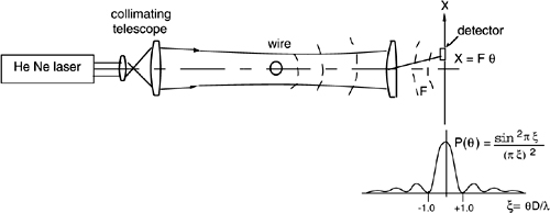
The wire to be measured is allowed to pass inside an aperture of the instrument, where it is illuminated by the beam waist of an expanded laser beam. As usual, we use a He-Ne laser and a collimating telescope (Fig. 2-13).

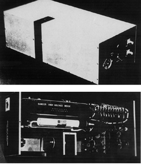
Fig. 2-13 A noncontact sensor for diameter measurement. Top: the instrument envelope, with the U-slit for wire passage; bottom: internal details include the He-Ne laser (center left), the collimating telescope (bottom left), the receiver (bottom right), and the electronics box (top left).

For the illuminating field, the wire is an obstruction or diffraction stop, and, in view of the Babinet principle, it is equivalent to a diffraction aperture. The diffracted field is collected by a lens (Fig.2-14) and its distribution is converted into an electrical signal by a photodetector placed in the focal plane of the lens. From this signal, the unknown diameter D can be calculated.

As well known from diffraction theory and recalled in App.A5, the distribution of diffraction from the wire is the Fourier transform of the wire aperture. Assuming a constant illuminating field E₀, the field and the radiant power density diffracted at the angle θ are given by (see Sect.A5.3):

(2.8)

(2.8’)

In these expressions, sinc ξ =(sin πξ)/πξ. The first zero of the sinc distribution is at ξ=±1, which corresponds to a diffraction angle θ_zero =±λ/D.

To work out D, we first manage to make available the P(θ) distribution and then look for the measurement strategy that is well suited to extract D from the distribution.

We use a lens (Fig.2-14) to convert the angular distribution P(θ) in a focal plane distribution P(X) to be scanned by the photodetector. The scale factor is X=Fθ, with F being the focal length of the lens.

Usually, we require a long focal length F for a sizeable X, yet we want to keep the overall length short (much less than F).

As an example, if D=200μm and λ=0.5μm, we need F=400 mm to have a zero at X=±1mm. A good choice is a telephoto lens [3] with two lenses, a front positive and a rear negative (or

Fig. 2-14 In a wire-diameter sensor, the wire is illuminated with a laser beam, properly expanded and collimated. The far-field distribution of diffracted light is converted by a lens to a spatial distribution in the focal plane. Scanning the focal plane by a photodetector reveals the zeros of the distribution, located at X/F=θ=± λ/D, hence the measurement of D.

Barlow’s focal multiplier). By this, an F=400 mm lens may be only 50-mm long.

On the source side (Fig.2-14), a collimating telescope is used to expand and collimate the laser beam, which makes a nearly plane wave front available in the measurement region. The size of the expanded beam D_beam is usually kept several mm to a few cm, according to user’s specifications.

With a larger size, a larger transversal movement is tolerated, and the errors associated to beam waist nonidealities are reduced. On the other hand, a larger size means less power on the wire and therefore a weaker signal and S/N ratio at the detector.

To measure D from the experimental distribution P(X)= P₀ sinc² XD/Fλ we may in principle look at several different features in the waveform P(X), for example, the main pulse width at half maximum, the secondary-maximum positions, the flex points, etc.

However, we shall take into account two nonidealities in the P(X) detection: (i) the finite size of the detector W_det, by which the P(X) distribution is averaged on W_det and (ii) the relatively strong peak coming from the non diffracted beam and superposed to the useful signal near the origin X=0 (this contribution is not shown in Fig.2-14).

If D_beam is the beam diameter at the waist illuminating the wire, the non diffracted peak has a width of the order of Fλ/D_beam and an amplitude D_beam²/D² times higher than the wire diffraction amplitude.

Then, a better feature to look at in the P(X) distribution is the location of the first zeroes near the peak. These are positioned at θ=±λ/D, or X=±Fλ/D. We may detect them conveniently with a linear-array Charge Coupled Device (CCD) [4] placed in the focal plane.

The CCD is a self-scanned detector, that provides a signal i(t)= i₀ sinc² vtD/Fλ, where v is the scanning speed. By time differentiating the signal i(t), we get an i’(t) signal, which passes through the zero level in correspondence to the minima of the sinc² function.

Further, we can arrange a digital processing of the measurement as follows: a threshold discrimination of the i’(t) signal picks up the zeroes at time t=±Fλ/vD and gates a counter to count clock transitions between two start and stop triggers. If the clock frequency is f_c, the number of counted pulses is N_count=2f_cFλ/vD, and we have a digital readout of the diameter D. However, we still require calculating a reciprocal.

In commercially available instruments, the range of measurable diameters extends from 10 μm to over 2 mm, and the corresponding accuracy is 1% and 5%, respectively, at the border of the measurement range.

Reasons for limits in the measurement are as follows. At large diameters, the diffraction angle becomes small, and the P(θ) is difficult to sort out, whereas errors due to illuminating wave front planarity and detector finite size become increasingly important. At the lower end of the diameter range, where diffraction angle is conveniently large, limits are due to the approximations in P(θ) and to vignetting-effect in the collecting lenses. It is worth noting that user’s specifications set a requirement on small diameter at ≈50 μm because very small wires are uncommon in industrial manufacturing.

In commercially available instruments, the allowed transversal movement of the wire is typically 2 to 5 mm with no degradation of other specifications. A typical overall size of the diameter-sensing instrument (Fig.2-14) is 50 by 20 by 10 cm.

2.5 Particle Sizing

Another instrument based on diffraction is the particle-size analyzer. With this instrument, we can measure the distribution of particle diameters in a fine-conglomerate mixture. A lot of mixtures are found interesting for particle sizing, ranging from manufacturing and industrial processes (ceramic, cement, and alloys powders) to particulate monitoring in air and water and sorting of living material for medical and biological purposes.

The first particle-size analyzers date back to the 1970s [5]. They were developed originally to keep the size distribution of ceramic and alloy powders under control in industrial manufacturing. Since then, the field has steadily matured, and the new products accepted in a variety of applications. The measurement range now extends from the submicron particulate to relatively large particles, up to about 1 mm, that cover a variety of surrounding media, while accuracy and resolution are improved and the sample size is reduced.

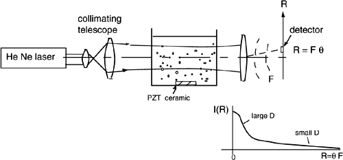
A basic scheme of a particle-size analyzer is shown in Fig.2-15. This scheme is similar to the wire sensor, and with it we look at the small-angle diffraction or elastic scattering of light from the particles. Because of this, the scheme is classified as Low-Angle Elastic Light Scattering (LAELS) [6].

As a source, we may use a low power (typically 5mW) semiconductor laser or He-Ne laser. The collimating telescope expands the beam and projects a nearly plane wave front on the measurement cell that contains the particles to be measured. In the cell, the particles are kept in suspension by means of a mechanical stirrer or an ultrasonic shaker (the PZT ceramic indicated in Fig.2-15). In this way, we avoid flocculation, or, the sticking together of particles.

Fig. 2-15 A particle-size analyzer is based on the diffraction of light projected on a cell containing the particles in a liquid suspension. At the output of the cell, a lens collects light diffracted at angle θ and converts it in a focal plane distribution I(R), with R=θF. Then, I(R) is measured by the photodetector, and the desired diameter distribution p(D) is computed.

If the cell is relatively thin, the wave front can be assumed plane throughout the cell, and particles are illuminated by the same wave vector. Each particle contributes to the far field distribution collected at the angle θ according to Fourier transform of an aperture of diameter D, as given by Eqs.A5-16 and A5.16’. The contribution is A₀ somb [(D/λ)sin θ] in field amplitude and I₀ somb²[(D/λ)sin θ] in power density, where somb x= 2J₁(πx)/πx (see App.A5.3). The total field amplitude and power density are the integrals of somb and somb² terms, weighted by p(D), the distribution of diameters in the particle ensemble.

In summing up the contributions, we shall recall that particles are randomly distributed in the cell, and their positions fluctuate well in excess of a wavelength. Because of this, the interference terms originated by the superposition of field amplitudes have zero average.

Thus, the square of the field sum is equal to the sum of the squares. In other words, in the far field of the cell, we shall add the intensities or the squares of the fields contributed by individual particles.

Using Eq.A5.16’ and integrating on the diameter distribution, the far field intensity I(θ) at the angle θ is written as:

(2.9)

Now, we want to calculate from Eq.2.9 the unknown distribution p(D) of particle size, after I(θ) is determined through a measurement of the far field intensity. The kernel of the Fredholm’s integral, somb²[(D/λ)sin θ], is a given term because we can compute it for any pair of given θ and D values.

However, the problem is known as an ill-conditioned one because p(D) is multiplied by the kernel, and the result is integrated on D so that details in p(D) are smoothed out in the result I(θ). For example, very large particles affect only a small interval in I(θ) near θ≈0, whereas very small ones give only a little increase of I(θ) at large θ.

Another source of error is the constant scattering coefficient tacitly assumed in writing Eq.2.9. This holds for large-particles, D>>λ, whereas for intermediate and small particles Q_ext varies appreciably (see Fig.A3-6 and Eq.A3.2).

From the previous considerations, the measurement range best suited for the LAELS will normally go from a few μm to perhaps several mm in diameter. At small D, the limit comes from the Rayleigh approximation, whereas at large diameter it depends on the size of the photodiode, due to measure at θ≈0 without disturbance from the undiffracted beam.

Because we are unable to solve Eq.2.9 exactly in all cases, we will try to maximize the information content picked out from the experiment through the measurements of I(θ). To do so, we will repeat the measurement at as many angles θ as the outcomes I(θ) are found appreciably different. With information provided by the I(θ) set, the kernel integral will limit resolution to a certain value, beyond which the solution becomes affected by a large oscillating error. We can then optimize the solution by increasing resolution (or number of diameters) until the computed p(D) starts being affected by oscillation errors.

Let us now briefly discuss the mathematical approaches that have been considered and applied to solve the inversion problem given by Eq.2.9.

Analytical Inversion. Although Eq.2.9 looks like intractable, Chin et al.[7] have been able to solve it for p(D) using hypergeometric functions, and the result is:

(2.10)

In this equation we have let K(x)= xJ₁(x)Y₁(x), J and Y are the usual Bessel functions, and d[.] =(∂[.]/∂θ) dθ are the differential of the product [.]=θ³I(.), in the variable θ.

Despite being a remarkable mathematical result, Eq.2.10 is difficult to use because it requires integrating I(θ) on θ from 0 to ∞. Unfortunately, the Fraunhofer approximation and the assumption of Rayleigh regime are valid only for θ≈0. To avoid an abrupt truncation of I(θ) and the resulting oscillation error in p(D), the data I(θ) is apodized to zero. A typical smoothing profile is P(θ)=1-(θ/θ_max)², and the maximum θ is chosen as θ_max≈(2-5)λ/D to cover the range of interest in diffraction.

In the range of diameter 10 to 50 μm and with λ =0.633 μm, the analytical inversion works nicely if measured data is very clean and accurate, that is, affected by an error of 1% or less.

Least Square Method. Using a discrete approximation, we may bring Eq.2.9 to a set of linear equations and then apply the Least-Square Method (LSM) to improve the stability of solution, i.e., reduce spurious oscillations.

To do so, we write the integral as a summation on the index k of the diameter variable D_k and repeat the equations for as many variables n of the angle of measurement θ_n. The matrix of known coefficients connecting θ_n and D_k is the discrete kernel S_nk:

(2.11)

The range of variables n and k is n=1..N and k=1..K, and the associated variables are I_n=I(θ_n) and p_k=p(D_k). With this, Eq.2.9 becomes:

(2.12)

In this set of equations, the number of equations N may be different from the number of unknown K. Usually, N is the number of angular measurements performed by the photodetector. If we use an array or a CCD to obtain a number of separate channels in angle θ, N is fixed and may be usually 50 to 100. The number of unknown diameters K is variable because we want to determine the calculated distribution p(D) on the largest number of separate diameters that are compatible with the absence of oscillating errors. Then usually we may have K=6-20, depending on the average D and the shape of p(D).

To solve for the unknown p_k, we need to bring the number of unknowns to coincide with the number of equations, whatever N and K are, and we do so by applying the LSM. With the LSM, we require that the solution p_k is such that the error ², or mean square deviation of the computed values ∑ S_nk p_k and measured ones I_n, is a minimum:

(2.13)

The condition of minimum is obtained by setting to zero the partial derivative of the error ², with respect to each value p_k of the unknown:

(2.13’)

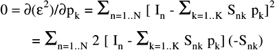
By rearranging the terms in this expression, we get:

(2.14)

where we have let:

(2.14’)

Now, the number of equations in 2.14 is equal to the number of unknowns and we can solve for p_k with standard algebra.

Using the LSM, the accuracy of solution improves, and the range of diameter distribution is larger with respect to the analytical inversion method. However, if data are affected by errors or the number of diameters is excessive, the error of the solution increases. Also, the error may be large if the waveform p(D) is bimodal or contains secondary peaks.

Thus, one has to choose a reasonable number of diameters to get the best result. A strategy is to increase the number K of diameters and repeat the calculation until in the new result oscillations or wrong features start to show up in the new result.

Usually, the range of diameter of interest may be large (for example, two decades from 2 to 200μm), but the number of affordable diameter is modest (e.g., K=6). Then, we get more information from the cumulative distribution P(D) than from the density function p(D). The relationship between the two is:

(2.15)

Of course, using Eq.2.15 with Eq.2.14 allows us to solve for P(D) with the LSM.

Errors in measured data I_n can be reduced by working on integral quantities in place of the differential ones considered so far. In fact, the photodetector has a finite area, and we usually strive to shrink its active aperture, but with a loss of signal-to-noise ratio. Then, it is better to start the problem of solving Eq.2.9 by assuming the signal is collected in a finite angular aperture θ₁ ..θ₂.

The integrated signal is written as if the photodetector is made of elements with the same area at all θ, or as if the photodetector is made of annulus elements for which the area increases with radius. In any case, by inserting Eq.2.9 in these expressions, we can integrate the kernel of the Fredholm’s integral, somb²[(D/λ)sin θ], with respect to θ, either numerically or analytically. The result, X(θ₁,θ₂), becomes X_nk when we use the discrete approximation, and this value can be used to solve for p_k or P_k with the LSM expressed by Eq.2.14.

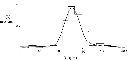
With this approach, monodispersed powders can be measured, in the range of diameter 20 to 50μm, typically with a <2% error, in K≈5 intervals of the cumulative distribution. At the expense of a reduced accuracy (≈5% error), the range can be extended to 5 to 200 μm and 7 to 10 intervals. A typical result of particle-size measurement is shown in Fig.2-16.

Fig. 2-16 Typical result of particle-size measurement as obtained by LAELS and LSM. Thick line: the true distribution, step-wise curve: the reconstructed distribution, dotted line: typical fluctuation for a 1% noise on data.

Other Linear Methods. The basic LSM we have outlined previously is the starting point for several extensions [8,9]. In all of them, we try to convey a physical constraint or information in a set of linear equations, just like the LSM concept leading to Eq.2.14.

A straight example is weighting of terms contributing to the total error ² in Eq.2.13. To do that, we may add, under the summation term of Eq.2.13, a multiplying factor w_n that is taken =1 where the measured I_n is clean (or, has a good S/N ratio), and <1 where I_n is noisy. Of course, the choice of the exact weight is somehow arbitrary or left to our knowledge of the powder nature. Accordingly, the quality (or error) of the results will depend on the w_n values we have chosen.

Other examples of information that may be added through linear equations are (i) the nonnegative character of the distribution p(D), which leads to an inversion method known as Non-Negative LSM (NNLSM); (ii) the known shape of the p(D) waveform, for example, monodispersed or bimodal; (iii) the minimum-ripple or smoothness constraint.

With the addition of the linear constraint, both accuracy and dynamic range of the reconstruction are significantly improved. However, linear methods have the general disadvantage of a success dependent on our ability to tune the added information and to adjust free parameters describing it [7-9].

Iterative Methods. The prototype of these methods is Chahine’s method [6,10] which is used to invert Fredholm’s equation in a variety of applications. We start letting K=N, that is, using a number of unknown variables p_k equal to the number of measured intensities I_n (K=N is also provided by the application of the LSM, first).

The iterative method is based on the following reasoning. If the set of diameter distribution p_k is correct, it should give the measured distribution I_n.calc= ∑_kC_nkp_k. If the set of calculated values I_n.calc differs from the experimental values, we may expect to approach the solution by multiplying p_k by I_k.meas/I_k.calc, where I_k.meas is the measured value, or explicitly:

(2.16)

By repeating the procedure an adequate number of times, p_k should converge to the correct solution. As a trial value of p_k, we can use either an estimated distribution or the result of a LSM calculation. Starting with an all-positive trial distribution, the results in all the iterations are necessarily positive, and we get the inherent benefit of suppressing oscillations with negative swings. The results obtained by the Chahine’s method are definitely better than the normal LSM. Errors are greatly reduced (by a factor 3 to 5), and the range of diameters is significantly increased. On the other hand, the tendency exists to generate spurious spikes at small D, unfortunately, in place of the oscillations suppressed by the method.

Another problem with Chahine’s and other iteration methods is that no clear sign exists when the optimal result is reached. Thus, we usually define a quality function, for example, the error ² of calculated results to measured ones, and stop the iteration when a minimum of ² is reached.

A refinement of Chahine’s method has been recently introduced [6]. It consists in weighting the iteration by the normalized kernel, S_nk/∑_n=1..NS_nk. With this position, Eq.2.16 reads:

(2.16’)

At the generic iteration, each term p_k is weighted by S_nk, that is, proportionally to the efficiency of transfer of p_k to the output I_n. In consequence, spurious peaks found in Chahine’s method are suppressed, and resolution and dynamic range are improved further [6].

With regard to the optical layout of the particle-size analyzer, several sources of error can influence the results. The finite size of the photodetector has already been considered, and found that it can be accounted for by reformulating Eq.2.8 in terms of integrated intensity.

Another error comes from the undiffracted beam at θ=0, which requires a stop on the focal plane to be blocked out (the stop is omitted in Fig.2-15 to avoid confusion). Even using the stop, some light will inevitably scatter or leak aside on the detector, which affects the θ≈0 measurements.

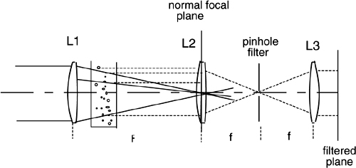
To get rid of it, we can use the filtering arrangement reported in Fig.2-17, known as reverse Fourier-transform illumination. Light projected through the cell by lens L1 converges at a focal plane position. The contribution diffracted at the angle θ reaches the focal plane of L1 at position x=θF with rays parallel to the optical axis.

Instead of reading the intensity in the focal plane, we place a lens L2 there and perform a Fourier transform of the incoming angular distribution. All the θ-diffracted rays arriving parallel to the optical axis are focused on the axis of L2 (Fig.2-17), whereas undiffracted light arriving at an angle will reach the focal plane out of the axis. Placing a pinhole at the focal plane of L2, we can allow the diffracted contribution through and block out the undiffracted one. With another lens L3, we can then retransform the filtered distribution to one with rays parallel to the optical axis.

Because of the scattering suppression, the arrangement of Fig.2-17 is much better of a stop in the focal plane, and we can measure down to small angle θ (typ. <0.1mrad). Accordingly, the range of large diameters that can be reconstructed is expanded up to several hundred μm or even to the mm.

Fig. 2-17 Using a convergent beam to illuminate the cell, we are able to filter out the undiffracted beam more efficiently than with stops. Diffracted rays indicated by dotted lines are focused on axis and can pass through the pinhole, whereas undiffracted rays arrive out-of-axis and are blocked.

At the other end of the measurement range, that of large diffracted angle or small diameter, the errors are not only due to collection efficiency, vignetting, and the like, but also to the Fraunhofer approximation D>>λ. Errors start becoming significant at, say, D≈2-5λ, so the practical range of measurement for particle sizing based only on the LAELS is typically 2…500 μm.

We can extend the range of measurement on small particles by taking advantage of the Mie (D≈λ) and Rayleigh (D<<λ) scattering regimes. These are described by the appropriate scattering function f(θ) and extinction factor Q_ext (Appendix A3.1), which are known and can be calculated from Mie’s theory [11].

In the Rayleigh regime, the scattering is nearly isotropic in angle, and the extinction factor Q_ext varies as (D/λ)⁴. When D increases up to about D≈λ, the scattering function peaks forward, and the extinction factor increases up to ≈2-4 (see Fig.A3-6).

Now, we can supplement the LAELS measurement with a measurement of light scattered from the cell at a fixed angle, i.e., large enough to be out of the range of LAELS data.

For example, a choice is to look at the cell from θ≈45° so that the detector is safely away the undiffracted beam leak. To collect information on the particle size distribution, we now scan the wavelength instead of the diffraction angle. By varying the ratio D/λ, the extinction factor Q_ext (D,λ,n) varies and so does the scattered power too.

For a density distribution p(D) of diameter, and given an extinction factor Q_ext (D,λ,n) at the measurement wavelength λ, the power density collected within a solid angle Δ Ω around θ=45° is given by:

(2.17)

where f(θ) is the scattering function and Q_ext is the extinction factor defined in App. A3.1. Eq.2.17 is clearly the counterpart of Eq.2.9 for the case at hand of extinction-related measurement. All the previously discussed methods of inversion of the Fredholm’s integral (Eq.2.17) can now be repeated [6] on the variables D_k and λ_n.

This method of particle sizing is called Spectral Extinction Aerosol Sizing (SEAS). With the computation of the distribution p(D) from Eq.2.17, it goes down to 0.02–0.1μm as the minimum measurable size, whereas the maximum range overlaps the minimum of LAELS (≈ 2-5 μm).

About the source, we need one with a high radiance and a wide spectral emission because the minimum detectable signal depends on radiance, and the minimum measurable size depends on the shortest wavelength available. To cover the visible and UV range, a cheap choice is a halogen lamp with 3000 to 3300-K color temperature. The lamp output is colli-mated by a lens and filtered by a monochromator. The output beam can either be combined with the laser beam of the LAELS by means of a wavelength-selective beamsplitter or used as stand-alone source. The detector to be used is usually a photomultiplier (see Ref.[1], Chapter 4) which is well suited for the spectral range UV-visible, and provides the best sensitivity, even in the case of small particulate concentration.

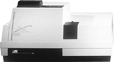
An example of a modern particle-sizing instrument is shown in Fig.2-18. This instrument is the technical evolution of a first product released in 1971.

A last method worth mentioning is the Dynamical Scattering Size Analyzer (DSSA), which is useful for measurements of very small (1..100-nm) particles [12]. Different from previous techniques, when particles are very small, the scattered light is frequency shifted. The shift is due to the Doppler effect (k_o-k_i)^.v, or equivalently by the interferometric phase (k_o-k_i)^.s, of the particle displacement s observed from the direction k_o and illuminated from k_I (all underlined quantities being intended vectors). The shift can be measured by a frequency-spectrum analysis or by a time-domain autocorrelation measurement of the detected signal. For example, the autocorrelation function is found to depend on the diffusion constant δ of the particles, as C(τ)=C₀ exp –δ (k_o-k_i)²τ. From the measurement of the exponential decay of C(τ), the diffusion constant is determined.

Then, we use the relation δ =kT/2πηD to determine the diameter D after the viscosity η of the particle in the surrounding medium is known.

Fig. 2-18 A modern particle-size analyzer based on diffraction and extinction performs diameter measurements from 0.05 to 2500 μm (courtesy of CILAS, France)

References

[1] S. Donati, “Photodetectors”, Prentice Hall: Upper Saddle River, 2000.

[2] R.D. Hudson, jr., “Infrared System Engineering”, Wiley Interscience: New York, 1969.

[3] D. Malacara and Z. Malacara, “Handbook of Lens Design”, Marcel Dekker Inc.: New York, 1994.

[4] see Ref.[1]. Section 9.4.

[5] J. Cornaillault, “Particle Size Analyzer”, Applied Optics vol.11 (1972), pp.265-269.

[6] F. Ferri, G. Righini, and E. Paganini, “Inversion of Low-Angle Elastic Light Scattering Data With a New Method Modifying Chanine Algorithm”, Applied Optics vol.36 (1997), pp.7539-50; see also: Applied Optics vol.34 (1995), pp.5829-5839.

[7] J.H. Chin, C.M. Sliepcevich, and M. Tribus, “An Improved Least Square Method Routine to Compute Particle Disatribution”, Journ. Phys. Chem. vol.56 (1955), pp.841-848.

[8] S. Twomey, “Introduction to Mathematics of Inversion in Remote Sensing and Indirect Measurements”, Elsevier: Amsterdam 1977, Chapter 7.

[9] N. Wolfson et al., “Comparative Study of Inversion Techniques, part I and part II’”, Applied Meteorology vol.18 (1979), pp.543-561.

[10] M.T. Chahine, “Determination of the Temperature Profile in an Atmosphere from its Outgoing Radiance”, Journal of Optical Soc. of Am. vol.58 (1968), pp.3074-3082.

[11] H.C. Van de Hulst, “Light Scattering by Small Particles”, J. Wiley: New York, 1957.

[12] B.J. Berne and R. Pecora, “Dynamic Light Scattering”, J. Wiley: New York, 1976.