Chapter 11 Nonisothermal Reactor Design-The Steady-State Energy Balance and Adiabatic PFR Applications

Search in book...
Toggle Font Controls
Create new playlist

Name your new playlist

Playlist description (optional)
Sign In

Email address

Password

Forgot Password?

or

Continue with Facebook

Continue with Google
Sign Up

Full Name

Email address

Confirm Email Address

Password

or

Continue with Facebook

Continue with Google

11. Nonisothermal Reactor Design—The Steady-State Energy Balance and Adiabatic PFR Applications

If you can’t stand the heat, get out of the kitchen.

—Harry S Truman

Overview. Because most reactions are not carried out isothermally, we now focus our attention on heat effects in chemical reactors. The basic CRE algorithm of mole balance, rate law, stoichiometry, combine, and evaluate used in Chapters 1 through 10 for isothermal reactor design is still valid for the design of nonisothermal reactors and we only need to add one more step, the energy balance to solve nonisothermal problems. The major difference lies in the method of evaluating the combined mole balances, rate law, and stoichiometry when temperature varies along the length of a PFR or when heat is removed from a CSTR. This chapter is arranged as follows:

• Section 11.1 shows why we need the energy balance and how it will be used to solve reactor design problems.

• Section 11.2 develops the energy balance to a point where it can be applied to different types of reactors. It then gives the end result, relating temperature and conversion or reaction rate for the main types of reactors we have been studying.

• Section 11.3 develops the user-friendly energy balances for reactors.

• Section 11.4 discusses the adiabatic operation of reactors.

• Section 11.5 shows how to determine the adiabatic equilibrium conversion and how to carry out interstage cooling.

• Section 11.6 closes the chapter with a discussion of the optimum inlet temperature to achieve the maximum conversion for adiabatic operation.

11.1 Rationale

To identify the additional information necessary to design nonisothermal reactors, we consider the following example, in which a highly exothermic reaction is carried out adiabatically in a plug-flow reactor.

Example 11-1 What Additional Information Is Required?

The first-order liquid-phase reaction

A → B

is carried out in a PFR. The reaction is exothermic and the reactor is operated adia-batically. As a result, the temperature will increase with conversion down the length of the reactor. Because T varies along the length of the reactor, k will also vary, which was not the case for isothermal plug-flow reactors.

Describe how to calculate the PFR reactor volume necessary for 70% conversion and plot the corresponding profiles for X and T.

Solution

The same CRE algorithm can be applied to nonisothermal reactions as to isothermal reactions by adding one more step, the energy balance.

1. Mole Balance (design equation):

d X d V = - r A F A 0 (E11-1.1)

$\begin{matrix} \frac{d X}{d V} = \frac{- r_{A}}{F_{A 0}} & \begin{matrix} (E11-1.1) \end{matrix} \end{matrix}$

2. Rate Law:

- r A = k C A (E11-1.2)

$\begin{matrix} - r_{A} = {k C}_{A} & (E11-1.2) \end{matrix}$

Recalling the Arrhenius equation, k = k₁ exp

k = k 1 exp [E R (1 T 1 - 1 T)] (E11-1.3)

$\begin{matrix} k = k_{1} \exp [\frac{E}{R} (\frac{1}{T_{1}} - \frac{1}{T})] & \begin{matrix} (E11-1.3) \end{matrix} \end{matrix}$

we know that k is a function of temperature, T.

3. Stoichiometry (liquid phase): υ = υ₀

C A = C A0 (1 - X) (E11-1.4)

$\begin{matrix} C_{A} = C_{A0} (1 - X) & (E11-1.4) \end{matrix}$

4. Combining:

- r A = k 1 exp [E R (1 T 1 - 1 T)] C A 0 (1 - X) (E11-1.5)

$\begin{matrix} - r_{A} = k_{1} \exp [\frac{E}{R} (\frac{1}{T_{1}} - \frac{1}{T})] C_{A 0} (1 - X) & \begin{matrix} (E11-1.5) \end{matrix} \end{matrix}$

Following the Algorithm

Combining Equations (E11-1.1), (E11-1.2), and (E11-1.4), and canceling the entering concentration, C_A0, yields

d X d V = k ( 1 - X ) v 0 (E11-1.6)

$\begin{matrix} \frac{d X}{d V} = \frac{k (1 - X)}{v_{0}} & (E11-1.6) \end{matrix}$

Combining Equations (E11-1.3) and (E11-1.6) gives us

d X d V = k 1 exp [E R (1 T 1 - 1 T)] 1 - X v 0 (E11-1.7)

$\begin{matrix} \frac{d X}{d V} = k_{1} \exp [\frac{E}{R} (\frac{1}{T_{1}} - \frac{1}{T})] \frac{1 - X}{v_{0}} & \begin{matrix} (E11-1.7) \end{matrix} \end{matrix}$

Oops! We see that we need another relationship relating X and T or T and V to solve this equation. The energy balance will provide us with this relationship.

So we add another step to our algorithm; this step is the energy balance.

5. Energy Balance:

In this step, we will find the appropriate energy balance to relate temperature and conversion or reaction rate. For example, if the reaction is adiabatic, we will show that for equal heat capacities, C_PA and C_PB , and a constant heat of reaction, ΔH∘Rx, $Δ H_{Rx}^{°},$ the temperature-conversion relationship can be written in a form such as

T = T 0 + - Δ H \circ R x C P A X (E11-1.8)

$\begin{matrix} T = T_{0} + \frac{- Δ H_{R x}^{\circ}}{C_{P_{A}}} X & \begin{matrix} (E11-1.8) \end{matrix} \end{matrix}$

We now have all the equations we need to solve for the conversion and temperature profiles. We simply type Equations (E11-1.7) and (E11-1.8) along with the parameters into Polymath, Wolfram, or MATLAB; click the RUN button; and then carry out the calculation to a volume where 70% conversion is obtained.

Analysis: The purpose of this example was to demonstrate that for nonisothermal chemical reactions we need another step in our CRE algorithm, the energy balance. The energy balance allows us to solve for the reaction temperature, which is necessary in evaluating the specific reaction rate constant k(T).

Why we need the energy balance

T₀ = Entering Temperature

ΔH_Rx = Heat of Reaction

C_{P_A} = Heat Capacity of species A

11.2 The Energy Balance

11.2.1 First Law of Thermodynamics

We begin with the application of the first law of thermodynamics, first to a closed system and then to an open system. A system is any bounded portion of the universe, moving or stationary, which is chosen for the application of the various thermodynamic equations. For a closed system, in which no mass crosses the system boundaries, the change in total energy of the system, dE, is equal to the heat flow to the system, SQ, minus the work done by the system on the surroundings, SW. For a closed system, the energy balance is

d E ˆ = δ Q - δ W (11-1)

$\begin{matrix} d \hat{E} = δ Q - δ W & \begin{matrix} (11-1) \end{matrix} \end{matrix}$

The δ’s signify that SQ and SW are not exact differentials of a state function.

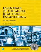
The continuous-flow reactors we have been discussing are open systems in which mass crosses the system boundary. We shall carry out an energy balance on the open system shown in Figure 11-1. For an open system in which some

Schematic shows a well-mixed open system. A downward arrow at the top center is labeled Q dot. The blades labeled W dot subscript s. A rightward arrow at the left is labeled F subscript i over in (example, F subscript A0): Hi over in (example, H subscript (A0)). A rightward arrow at the right is labeled F subscript i over out (example, F subscript A): Hi over out (example, H subscript A).

Figure 11-1 Energy balance on a well-mixed open system: schematic.

of the energy exchange is brought about by the flow of mass across the system boundaries, the energy balance for the case of only one species entering and leaving becomes

⎡⎣⎢⎢⎢⎢⎢⎢Rate ofaccumulationof energywithin thesystem⎤⎦⎥⎥⎥⎥⎥⎥dEˆsysdt(J/s)===⎡⎣⎢⎢⎢⎢⎢⎢Rate of flowof heat tothe systemfrom thesurroundings⎤⎦⎥⎥⎥⎥⎥⎥Q˙(J/s)−−−⎡⎣⎢⎢⎢⎢⎢⎢Rate of flowdone bythe systemon thesurroundings⎤⎦⎥⎥⎥⎥⎥⎥W˙(J/s)+++⎡⎣⎢⎢⎢⎢⎢⎢Rate of energyadded to thesystem by massflow into thesystem⎤⎦⎥⎥⎥⎥⎥⎥FinEin(J/s)−−−⎡⎣⎢⎢⎢⎢⎢⎢Rate ofenergy leavingthe system by massflow out ofthe system⎤⎦⎥⎥⎥⎥⎥⎥FoutEout(11-2)(J/s) $\begin{array}{l} [\begin{matrix} Rate of \\ accumulation \\ of energy \\ within the \\ system \end{matrix}] & = & [\begin{matrix} Rate of flow \\ of heat to \\ the system \\ from the \\ surroundings \end{matrix}] & - & [\begin{matrix} Rate of flow \\ done by \\ the system \\ on the \\ surroundings \end{matrix}] & + & [\begin{matrix} Rate of energy \\ added to the \\ system by mass \\ flow into the \\ system \end{matrix}] & - & [\begin{matrix} Rate of \\ energy leaving \\ the system by mass \\ flow out of \\ the system \end{matrix}] \\ \frac{d {\hat{E}}_{sys}}{dt} & = & \dot{Q} & - & \dot{W} & + & F_{in} E_{in} & - & \begin{matrix} \begin{matrix} F_{out} E_{out} \end{matrix} & (11-2) \end{matrix} \\ (J/s) & = & (J/s) & - & (J/s) & + & (J/s) & - & (J/s) \end{array}$

Energy balance on an open system

Typical units for each term in Equation (11-2) are (Joule/s). (Joule bio: http://www.corrosion-doctors.org/Biographies/JouleBio.htm.)

We will assume that the contents of the system volume are well mixed, an assumption that we could relax but that would require a couple of pages of text to develop, and the end result would be the same! The unsteady-state energy balance for an open well-mixed system that now has n species, each entering and leaving the system at its respective molar flow rate F_i (moles of i per time) and with its respective energy E_i (Joules per mole of i), is

d E ˆ sys d t = Q ˙ - W ˙ + \sum i = 1 n E i F i ∣ ∣ ∣ in - \sum i = 1 n E i F i ∣ ∣ ∣ out (11 - 3)

$\begin{array}{l} \frac{d {\hat{E}}_{sys}}{d t} = \dot{Q} - \dot{W} + \sum_{i = 1}^{n} E_{i} F_{i} {|_{in} - \sum_{i = 1}^{n} E_{i} F_{i} |}_{out} & (11 - 3) \end{array}$

We will now discuss each of the terms in Equation (11-3).

The starting point

11.2.2 Evaluating the Work Term

It is customary to separate the work term, W˙ $\dot{W}$ , into flow work and other work, W˙s ${\dot{W}}_{s}$ . The term W˙s ${\dot{W}}_{s}$ , often referred to as the shaft work, could be produced from such things as a stirrer in a CSTR or a turbine in a PFR. Flow work is work that is necessary to get the mass into and out of the system. For example, when shear stresses are absent, we write

W˙=−∑i=1nFiPV˜i∣∣∣in+∑i=1nFiPV˜i∣∣∣out+W˙s[Rate of flow work](11-4) $\begin{matrix} \dot{W} = \overset{[Rate of flow work]}{\overset{︷}{- \sum_{i = 1}^{n} F_{i} P {\tilde{V}}_{i} |_{in} + \sum_{i = 1}^{n} F_{i} P {\tilde{V}}_{i} |_{out} + {\dot{W}}_{s}}} & (11-4) \end{matrix}$

where P is the pressure (Pa) [1 Pa = 1 Newton/m² = 1 kg·m/s²/m²] and V˜i ${\tilde{V}}_{i}$ is the specific molar volume of species i (m³/mol of i).

Flow work and shaft work

Let’s look at the units of the flow-work term, which is

F i \cdot P \cdot V ˜ i

$F_{i} \cdot P \cdot {\tilde{V}}_{i}$

where F¡ is in mol/s, P is in Pa (1 Pa = 1 Newton/m²), and V˜i ${\tilde{V}}_{i}$ is in (m³/mol). Multiplying the units of each term in (FiPV˜i $F_{i} P {\tilde{V}}_{i}$ ) through, we obtain the units of flow work, i.e.,

F i \cdot P \cdot V ˜ i [=] mol s \cdot Newton m 2 \cdot m 3 mol = (N e w t o n \cdot m) \cdot 1 s = Joules/s = Watts

$F_{i} \cdot P \cdot \tilde{V}_{i} [=] \frac{mol}{s} \cdot \frac{Newton}{m^{2}} \cdot \frac{m^{3}}{mol} = (N e w t o n \cdot m) \cdot \frac{1}{s} = Joules/s = Watts$

We see that the units for flow work are consistent with the other terms in Equation (11-3), i.e., J/s (http://www.corrosion-doctors.org/BiographiesfWattBio.htm).

In most instances, the flow-work term is combined with those terms in the energy balance that represent the energy exchange by mass flow across the system boundaries. Substituting Equation (11-4) into (11-3) and grouping terms, we have

d E ˆ sys d t = Q ˙ - W ˙ s + \sum i = 1 n F i (E i + P V ˜ i) ∣ ∣ ∣ ∣ in - \sum i = 1 n F i (E i + P V ˜ i) ∣ ∣ ∣ ∣ out (11-5)

$\begin{matrix} \frac{d {\hat{E}}_{sys}}{d t} = \dot{Q} - {\dot{W}}_{s} + \sum_{i = 1}^{n} F_{i} (E_{i} + P {\tilde{V}}_{i}) |_{in} - \sum_{i = 1}^{n} F_{i} (E_{i} + P {\tilde{V}}_{i}) |_{out} & \begin{matrix} (11-5) \end{matrix} \end{matrix}$

The energy F¡ is the sum of the internal energy (U_i), the kinetic energy (u2i/2 $u_{i}^{2} / 2$ ), the potential energy (gz_i), and any other energies, such as electric or magnetic energy or light

E i = U i + u 2 i 2 + g z i + other (11-6)

$\begin{matrix} E_{i} = U_{i} + \frac{u_{i}^{2}}{2} + {g z}_{i} + other & \begin{matrix} (11-6) \end{matrix} \end{matrix}$

In almost all chemical reactor situations, the kinetic, potential, and “other” energy terms are negligible in comparison with the enthalpy, heat transfer, and work terms, and hence will be omitted, in which case

E i = U i (11-7)

$\begin{matrix} E_{i} = U_{i} & \begin{matrix} (11-7) \end{matrix} \end{matrix}$

We recall that the enthalpy, H_i (J/mol), is defined in terms of the internal energy U_i (J/mol), and the product PV_i (1 Pa·m³/mol = 1 J/mol):

H i = U i + P V ˜ i (11-8)

$\begin{matrix} H_{i} = U_{i} + {P \tilde{V}}_{i} & \begin{matrix} (11-8) \end{matrix} \end{matrix}$

Convention Heat Added Q˙ $\dot{Q}$ = +10J/s

Heat Removed Q˙ $\dot{Q}$ = −10J/s

Work Done by System W˙s ${\dot{W}}_{s}$ = +10J/s

Work Done on System W˙s ${\dot{W}}_{s}$ = −10J / s

Enthalpy

Typical units of H_i are

(H i) = J mol i or But lb-mol i or cal mol i

$(H_{i}) = \frac{J}{mol i} or \frac{But}{lb-mol i} or \frac{cal}{mol i}$

Enthalpy carried into (or out of) the system can be expressed as the sum of the internal energy carried into (or out of) the system by mass flow plus the flow work:

F i H i = F i (U i + P V ˜ i)

$F_{i} H_{i} = F_{i} (U_{i} + {P \tilde{V}}_{i})$

Combining Equations (11-5), (11-7), and (11-8), we can now write the energy balance in the form

d E ˆ sys d t = Q ˙ - W ˙ s + \sum i = 1 n F i H i ∣ ∣ ∣ ∣ in - \sum i = 1 n F i H i ∣ ∣ ∣ ∣ out

$\frac{{d \hat{E}}_{sys}}{d t} = \dot{Q} - {\dot{W}}_{s} + \sum_{i = 1}^{n} F_{i} H_{i} |_{in} - \sum_{i = 1}^{n} F_{i} H_{i} |_{out}$

The energy of the system at any instant in time, Ê_sys, is the sum of the products of the number of moles of each species in the system multiplied by their respective energies. The derivative of the E_sys term wrt time will be discussed in more detail when unsteady-state reactor operation is considered in Chapter 13.

We shall let the subscript “0” represent the inlet conditions. The conditions at the outlet of the chosen system volume will be represented by the unsubscripted variables.

Q ˙ - W ˙ S + \sum ​ i = 1 n F i 0 H i 0 - \sum ​ i = 1 n F i H i = d E ˆ sys d t (11 - 9)

$\begin{array}{l} \dot{Q} - {\dot{W}}_{S} + {\sum^{}}_{i = 1}^{n} F_{i 0} H_{i 0} - {\sum^{}}_{i = 1}^{n} F_{i} H_{i} = \frac{d {\hat{E}}_{sys}}{d t} & (11 - 9) \end{array}$

In Section 11.1, we discussed that in order to solve reaction engineering problems with heat effects, we needed to relate temperature, conversion, and rate of reaction. The energy balance as given in Equation (11-9) is the most convenient starting point as we proceed to develop this relationship.

Energy Balance

Figure resembles a well-balanced see-saw. A downward arrow labeled in, pointing to the left part, reads: F subscript (i0) H subscript (i0), Q dot. An upward arrow labeled out, pointing to the right part, reads: F subscript (i) H subscript (i), W subscript s dot.

11.2.3 Overview of Energy Balances

What is the plan? In the following pages we manipulate Equation (11-9) in order to apply it to each of the reactor types we have been discussing: BR, PFR, PBR, and CSTR. The end result of the application of the energy balance to each type of reactor is shown in Table 11-1. These equations can be used in Step 5 of the algorithm discussed in Example E11-1. The equations in Table 11-1 relate temperature to conversion and to molar flow rates, and to the system parameters, such as the product of overall heat-transfer coefficient, U, and heat exchange surface area, a, i.e., Ua, with the corresponding ambient temperature, T_a, and the heat of reaction, ΔH_Rx.

Examples of How to Use Table 11-1.

We now couple the energy balance equations in Table 11-1 with the appropriate reactor mole balance, rate law, and stoichiometry algorithm to solve reaction engineering problems with heat effects.

TABLE 11-1 ENERGY BALANCES OF COMMON REACTORS

1. Adiabatic (Q˙≡0 $\dot{Q} \equiv 0$ ) CSTR, PFR, Batch, or PBR. The relationship between conversion calculated from the energy balance, X_EB, and temperature for W˙s=0 ${\dot{W}}_{s} = 0$ , constant Cpi $C_{p_{i}}$ , and ΔCp=0 $Δ C_{p} = 0$ , is

Conversion in terms of temperature

X EB = \sum Θ i C P i ( T - T 0 ) - Δ H \circ Rx (T 11 - 1. A)

$\begin{array}{l} X_{EB} = \frac{\sum Θ_{i} C_{P_{i}} (T - T_{0})}{- Δ H_{Rx}^{\circ}} & (T 11 - 1. A) \end{array}$

Temperature in terms of conversion calculated from the energy balance

T = T 0 + ( - Δ H \circ Rx ) X EB Σ Θ i C P i (T 11 - 1. B)

$\begin{array}{l} T = T_{0} + \frac{(- Δ H_{Rx}^{\circ}) X_{EB}}{Σ Θ_{i} C_{P_{i}}} & (T 11 - 1. B) \end{array}$

For an exothermic reaction (−H_Rx) > 0

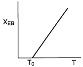
Graph shows a horizontal axis, T, a vertical axis, X subscript (EB), and a line that starts from a point T subscript 0 and rises.

2. CSTR with heat exchanger, UA (T_a − T), and large coolant flow rate

Schematic shows a vertical cylinder. A rightward arrow from the cylinder is labeled T. A downward arrow points to the cylinder. A heat exchanger from m subscript C dot to T subscript a is shown.

3. PFR/PBR with heat exchange

Schematic shows a tube within a horizontal cylinder on the left and right.

In general most of the PFR and PBR energy balances can be written as

d T d V = ( Heat “generated” ) - ( Heat “removed” ) Σ F i C P i = Q g - Q r Σ F i C P i

$\frac{d T}{d V} = \frac{(Heat “generated”) - (Heat “removed”)}{Σ F_{i} C_{P_{i}}} = \frac{Q_{g} - Q_{r}}{Σ F_{i} C_{P_{i}}}$

3A. PFR in terms of conversion

d T d V = r A Δ H Rx ( T ) Q g 0000 - U a ( T - T a ) Q r 0000 F A0 ( Σ Θ i C P i + Δ C P X ) = Q g - Q r F A0 ( Σ Θ i C P i + Δ C P X ) (T 11 - 1. D)

$\begin{array}{l} \frac{d T}{d V} = \frac{\overset{\underset{}{Q_{g}}}{r_{A} Δ H_{Rx} (T)} - \overset{\underset{}{Q_{r}}}{U a (T - T_{a})}}{F_{A0} (Σ Θ_{i} C_{P_{i}} + Δ C_{P} X)} = \frac{Q_{g} - Q_{r}}{F_{A0} (Σ Θ_{i} C_{P_{i}} + Δ C_{P} X)} & (T 11 - 1. D) \end{array}$

3B. PBR in terms of conversion

d T d W = r ' A Δ H Rx ( T ) - U a ρ b ( T - T a ) F A0 ( Σ Θ i C P i + Δ C P X ) (T 11 - 1. E)

$\begin{array}{l} \frac{d T}{d W} = \frac{{r^{'}}_{A} Δ H_{Rx} (T) - \frac{U a}{ρ_{b}} (T - T_{a})}{F_{A0} (Σ Θ_{i} C_{P_{i}} + Δ C_{P} X)} & (T 11 - 1. E) \end{array}$

3C. PBR in term of molar flow rates

d T d W = r ' A Δ H Rx ( T ) - U a ρ b ( T - T a ) Σ F i C P i (T 11 - 1. F)

$\begin{array}{l} \frac{d T}{d W} = \frac{{r^{'}}_{A} Δ H_{Rx} (T) - \frac{U a}{ρ_{b}} (T - T_{a})}{Σ F_{i} C_{P_{i}}} & (T 11 - 1. F) \end{array}$

3D. PFR in term of molar flow rates

d T d W = r A Δ H Rx ( T ) - U a ( T - T a ) Σ F i C P i = Q g - Q r Σ F i C P i (T 11 - 1. G)

$\begin{array}{l} \frac{d T}{d W} = \frac{r_{A} Δ H_{Rx} (T) - U a (T - T_{a})}{Σ F_{i} C_{P_{i}}} = \frac{Q_{g} - Q_{r}}{Σ F_{i} C_{P_{i}}} & (T 11 - 1. G) \end{array}$

4. Batch

d T d W = ( r A V ) ( Δ H Rx ) - U A ( T - T a ) Σ N i C P i (T 11 - 1. H)

$\begin{array}{l} \frac{d T}{d W} = \frac{(r_{A} V) (Δ H_{Rx}) - U A (T - T_{a})}{Σ N_{i} C_{P_{i}}} & (T 11 - 1. H) \end{array}$

5. For Semibatch or unsteady CSTR

d T d W = Q ˙ - W ˙ s - \sum i = 1 n F i 0 C P i ( T - T i 0 ) + [ - Δ H R x ( T ) ] ( - r A V ) \sum i = 1 n N i C P i (T 11 - 1. H)

$\begin{array}{l} \frac{d T}{d W} = \frac{\dot{Q} - {\dot{W}}_{s} - \sum_{i = 1}^{n} F_{i 0} C_{P_{i}} (T - T_{i 0}) + [- Δ H_{R x} (T)] (- r_{A} V)}{\sum_{i = 1}^{n} N_{i} C_{P_{i}}} & (T 11 - 1. H) \end{array}$

6. For multiple reactions in a PFR (q reactions and m species)

d T d V = \sum i = 1 q r i j Δ H Rx i j - U a ( T - T a ) \sum j = 1 m F j C P j (T 11 - 1. J)

$\begin{array}{l} \frac{d T}{d V} = \frac{\sum_{i = 1}^{q} r_{i j} Δ H_{Rx i j} - U a (T - T_{a})}{\sum_{j = 1}^{m} F_{j} C_{P_{j}}} & (T 11 - 1. J) \end{array}$

i = reaction number, j = species

7. Variable heat exchange fluid temperature, T_a

Co-current Exchange

d T a d V = U a ( T - T a ) m ˙ c C P c V = 0 T a = T a 0 (T 11 - 1. K)

$\begin{array}{l} \frac{d T_{a}}{d V} = \frac{U a (T - T_{a})}{{\dot{m}}_{c} C_{P_{c}}} \\ \begin{array}{l} V = 0 T_{a} = T_{a 0} & (T 11 - 1. K) \end{array} \end{array}$

Countercurrent Exchange

d T a d V = U a ( T a - T ) m ˙ c C P c V = V final T a = T a 0 (T 11 - 1. L)

$\begin{array}{l} \frac{d T_{a}}{d V} = \frac{U a (T_{a} - T)}{{\dot{m}}_{c} C_{P_{c}}} \\ \begin{array}{l} V = V_{final} T_{a} = T_{a 0} & (T 11 - 1. L) \end{array} \end{array}$

The equations in Table 11-1 are the ones we will use to solve reaction engineering problems with heat effects.

Nomenclature:

U = overall heat-transfer coefficient, (J/m² · s · K);

A = CSTR heat-exchange area, (m²);

a = PFR heat-exchange area per volume of reactor, (m²/m³);

CPi $C_{P}_{_{i}}$ = mean heat capacity of species i, (J/mol/K);

CPc $C_{P}_{_{c}}$ = the heat capacity of the coolant, (J/kg/K);

m˙c ${\dot{m}}_{c}$ = coolant flow rate, (kg/s);

ΔHRx(T) $Δ H_{Rx} (T)$ = heat of reaction at temperature T, (J/mol A):

ΔH∘Rx=(daH∘D+caH∘C−baH∘B−H∘A)J/mol A $Δ H_{Rx}^{\circ} = (\frac{d}{a} H_{D}^{\circ} + \frac{c}{a} H_{C}^{\circ} - \frac{b}{a} H_{B}^{\circ} - H_{A}^{\circ}) J/mol A$ = heat of reaction at temperature T_R;

ΔHRxij $Δ H_{Rx i j}$ = heat of reaction wrt species j in reaction i, (J/mol j):

Q˙ $\dot{Q}$ = heat added to the reactor, (J/s); and

ΔCP=(daCPD+caCPC−baCPB−CPA)(J/mol⋅K). $Δ C_{P} = (\frac{d}{a} C_{P_{D}} + \frac{c}{a} C_{P_{C}} - \frac{b}{a} C_{P_{B}} - C_{P_{A}}) (J / mol · K) .$

All other symbols are as defined in Chapters 1 through 10.

End results of manipulating the energy balance (Sections 11.2.4, 12.1, and 12.3)

For example, recall the rate law for a first-order reaction, Equation (E11-1.5) in Example 11-1

- r A = k 1 exp [E R (1 T 1 - 1 T)] C A0 (1 - X) (E11-1.5)

$\begin{matrix} - r_{A} = k_{1} exp [\frac{E}{R} (\frac{1}{T_{1}} - \frac{1}{T})] C_{A0} (1 - X) & \begin{matrix} (E11-1.5) \end{matrix} \end{matrix}$

which will be combined with the mole balance to find the concentration, conversion and temperature profiles (i.e., BR, PBR, PFR), exit concentrations, and conversion and temperature in a CSTR. We will now consider four cases of heat exchange in a PFR and PBR: (1) adiabatic, (2) co-current, (3) countercur-rent, and (4) constant exchanger fluid temperature. We focus on adiabatic operation in this chapter and the other three cases in Chapter 12.

Case 1: Adiabatic. If the reaction is carried out adiabatically, then we use Equation (E11-1.3) for the reaction A−→−−000000B $A \overset{}{\to} B$ in Example 11-1 to obtain

T = T 0 + - Δ H \circ Rx X C P A (T11-1.B)

$\begin{matrix} T = T_{0} + \frac{- Δ H_{Rx}^{\circ} X}{C_{P_{A}}} & (T11-1.B) \end{matrix}$

Adiabatic

Consequently, we can now obtain –r_A as a function of X alone by first choosing X, then calculating T from Equation (T11-1.B), then calculating k from Equation (E11-1.3), and then finally calculating (−r_A) from Equation (E11-1.5).

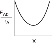
Choose X \to calculate T \to calculate k \to calculate - r A \to calculate F A0 - r A

$Choose X \to calculate T \to calculate k \to calculate - r_{A} \to calculate \frac{F_{A0}}{- r_{A}}$

We can use this sequence to prepare a table of (F_A0/−r_A) as a function of X. We can then proceed to size PFRs and CSTRS. In the absolute worst case scenario, we could use the techniques in Chapter 2 (e.g., Levenspiel plots or the quadrature formulas in Appendix A). However, instead of using a Levenspiel plot, we will most definitely use Polymath to solve our coupled differential energy and mole balance equations.

The algorithm

Graph shows a horizontal axis labeled X, a vertical axis labeled negative (F subscript (A0) over (negative r subscript A)), and an upward open parabolic curve.

Levenspiel plot

Cases 2, 3, and 4: Correspond to Co-current Heat Exchange, Countercurrent Heat Exchange, and Constant Coolant Temperature T_C, respectively (Ch. 12). If there is cooling along the length of a PFR or PBR, we could then apply Equation (T11-1.D) to this reaction to arrive at two coupled differential equations.

d X d V = k 1 exp [E R (1 T 1 - 1 T)] C A0 (1 - X) / F A0 d T d V = r A Δ H Rx ( T ) - U a ( T - T a ) F A0 C P A

$\begin{matrix} \frac{d X}{d V} = & k_{1} exp [\frac{E}{R} (\frac{1}{T_{1}} - \frac{1}{T})] C_{A0} (1 - X) / F_{A0} \\ \frac{d T}{d V} = \frac{r_{A} Δ H_{Rx} (T) - U a (T - T_{a})}{F_{A0} C_{P_{A}}} \end{matrix}$

Non-adiabatic PFR

which are easily solved using an ODE solver such as Polymath. If the temperature of the heat exchanger fluid (T_a) (e.g., coolant) is not constant, we add Equations (T11-1.K) or (T11-1.L) in Table 11-1 to the above equations and solve with Polymath, Wolfram, or MATLAB.

Heat Exchange in a CSTR. Similarly, for the case of the reaction A — B in Example 11-1 carried out in a CSTR, we could use Polymath or MATLAB to solve two nonlinear algebraic equations in X and T. These two equations are the combined mole balance

V = F A0 X k 1 exp [ E R ( 1 T 1 - 1 T ) ] C A0 ( 1 - X )

$\begin{matrix} V = & \frac{F_{A0} X}{k_{1} \exp [\frac{E}{R} (\frac{1}{T_{1}} - \frac{1}{T})] C_{A0} (1 - X)} \end{matrix}$

Non-adiabatic CSTR

and the application of Equation (T11-1.C), which is rearranged in the form

T = F A0 X ( - Δ H Rx ) + U A T a + F A0 C P A T 0 U A + C P A F A0

$T = \frac{F_{A0} X (- Δ H_{Rx}) + U A T_{a} + F_{A0} C_{P_{A}} T_{0}}{U A + C_{P_{A}} F_{A0}}$

From these three cases, (1) adiabatic PFR and CSTR, (2) PFR and PBR with heat effects, and (3) CSTR with heat effects, one can see how to couple the energy balances and mole balances. In principle, one could simply use Table 11-1 to apply to different reactors and reaction systems without further discussion. However, understanding the derivation of these equations will greatly facilitate the proper application to and evaluation of various reactors and reaction systems. Consequently, we now derive the equations given in Table 11-1.

Why bother to derive the equations in Table 11-1? Because I have found that students can apply these equations much more accurately to solve reaction engineering problems with heat effects if they have gone through the derivation to understand the assumptions and manipulations used in arriving at the equations in Table 11.1, That is, understanding these derivations, students are more likely to put the correct number in the correct equation symbol.

Why bother? Here is why!!

11.3 The User-Friendly Energy Balance Equations

We will now dissect the molar flow rates and enthalpy terms in Equation (11-9) to arrive at a set of equations we can readily apply to a number of reactor situations.

11.3.1 Dissecting the Steady-State Molar Flow Rates to Obtain the Heat of Reaction

To begin our journey, we start with the energy balance Equation (11-9), and then proceed to finally arrive at the equations given in Table 11-1 by first dissecting two terms:

1. The molar flow rates, F_i and F_i0

2. The molar enthalpies, H_i, H_i0[H_i = H_i(T), and H_i0 = H_i(T₀)]

Interactive

Schematic shows a PC with arrows shooting from it toward all the four directions.

Computer Modules

An animated and somewhat humorous version of what follows for the derivation of the energy balance can be found in the reaction engineering games “Heat Effects 1” and “Heat Effects 2” on the CRE Web site, http://www.umich.edu/~elements/5e/icm/index.html. Here, equations move around the screen, making substitutions and approximations to arrive at the equations shown in Table 11-1. Visual learners find these two ICGs a very useful resource (http://www.umich.edu/~elements/5e/icm/heatfx1.html).

We will now consider flow systems that are operated at steady state. The steady-state energy balance is obtained by setting (dÊ_sys/dt) equal to zero in Equation (11-9) in order to yield

Q ˙ - W ˙ s + \sum i = 1 n F i 0 H i 0 - \sum i = 1 n F i H i = 0 (11 - 10)

$\begin{array}{l} \dot{Q} - {\dot{W}}_{s} + \sum_{i = 1}^{n} F_{i 0} H_{i 0} - \sum_{i = 1}^{n} F_{i} H_{i} = 0 & (11 - 10) \end{array}$

Steady-state energy balance

To carry out the manipulations to write Equation (11-10) in terms of the heat of reaction, we shall use the generic reaction

A + b a B - \to - - 0000000 c a C + d a D (2-2)

$\begin{matrix} A + \frac{b}{a} B \overset{}{\to} \frac{c}{a} C + \frac{d}{a} D & \begin{matrix} (2-2) \end{matrix} \end{matrix}$

The inlet and outlet summation terms in Equation (11-10) are expanded, respectively, to

In: Σ Hi0Fi0=HA0FA0+HB0FB0+HC0FC0+HD0FD0+HI0FI0(11-11) $In: \begin{matrix} Σ H_{i 0} F_{i 0} = H_{A 0} F_{A 0} + H_{B 0} F_{B 0} + H_{C 0} F_{C 0} + H_{D 0} F_{D 0} + H_{I 0} F_{I 0} & \begin{matrix} (11-11) \end{matrix} \end{matrix}$

and

Out: Σ HiFi=HAFA+HBFB+HCFC+HDFD+HIFI(11-12) $\begin{matrix} Out: Σ H_{i} F_{i} = H_{A} F_{A} + H_{B} F_{B} + H_{C} F_{C} + H_{D} F_{D} + H_{I} F_{I} & (11-12) \end{matrix}$

where the subscript I represents inert species.

We next express the molar flow rates in terms of conversion. In general, the molar flow rate of species i for the case of no accumulation and a stoichiometric coefficient v_i is

F i = F A 0 (Θ i + v i X)

$F_{i} = F_{A 0} (Θ_{i} + v_{i} X)$

Specifically, for Reaction (2-2), A+baB−→−−000000caC+daD $A + \frac{b}{a} B \overset{}{\to} \frac{c}{a} C + \frac{d}{a} D$ , we have

F A = F A0 (1 - X) F B = F A0 (Θ B - b a X) F C = F A0 (Θ C - c a X) F D = F A0 (Θ D - d a X) F 1 = Θ 1 F A0 ⎫ ⎭ ⎬ ⎪ ⎪ ⎪ ⎪ ⎪ ⎪ ⎪ ⎪ ⎪ ⎪ ⎪ ⎪ ⎪ ⎪ ⎪ ⎪ ⎪ ⎪ ⎪ ⎪ where Θ i = F i 0 F A0

$\begin{array}{l} F_{A} = F_{A0} (1 - X) \\ \begin{array}{l} F_{B} = F_{A0} (Θ_{B} - \frac{b}{a} X) \\ F_{C} = F_{A0} (Θ_{C} - \frac{c}{a} X) \\ F_{D} = F_{A0} (Θ_{D} - \frac{d}{a} X) \\ F_{1} = Θ_{1} F_{A0} \end{array}} where Θ_{i} = \frac{F_{i 0}}{F_{A0}} \end{array}$

Steady-state operation

We can substitute these symbols for the molar flow rates into Equations (11-11) and (11-12), then subtract Equation (11-12) from (11-11) to give

\sum ​ i = 1 n F i 0 H i 0 - \sum ​ i = 1 n F i H i = F A 0 [(H A 0 - H A) + (H B 0 - H B) Θ B + (H C 0 - H C) Θ C + (H D 0 - H D) Θ D - (H I 0 - H I) Θ I] (- d a H D + c a H C - b a H B - H A)                                        Δ H R x F A 0 X (11 - 13)

$\begin{matrix} {\sum^{}}_{i = 1}^{n} F_{i 0} H_{i 0} - {\sum^{}}_{i = 1}^{n} F_{i} H_{i} = & F_{A 0} [(H_{A 0} - H_{A}) + (H_{B 0} - H_{B}) Θ_{B} \\ + (H_{C 0} - H_{C}) Θ_{C} + (H_{D 0} - H_{D}) Θ_{D} - (H_{I 0} - H_{I}) Θ_{I}] \\ \underset{Δ H_{R x}}{\underset{︸}{(- \frac{d}{a} H_{D} + \frac{c}{a} H_{C} - \frac{b}{a} H_{B} - H_{A})}} F_{A 0} X & (11 - 13) \end{matrix}$

The term in parentheses that is multiplied by F_A0X is called the heat of reaction at temperature T and is designated ΔH_Rx(T).

Δ H Rx (T)= d a H D (T)+ c a H C (T) - b a H B (T) - H A (T) (11 - 14)

$Δ H_{Rx} (T)= \frac{d}{a} H_{D} (T)+ \frac{c}{a} H_{C} (T) - \frac{b}{a} H_{B} (T) - H_{A} (T) (11 - 14)$

Heat of reaction at temperature T

All enthalpies (e.g., H_A, H_B) are evaluated at a temperature T in the reactor and, consequently, [ΔH_Rx(T)] is the heat of reaction at that specific temperature T. The heat of reaction is always given per mole of the species that is the basis of calculation, i.e., species A (Joules per mole of A reacted).

Substituting Equation (11-14) into (11-13) and reverting to summation notation for the species, Equation (11-13) becomes

\sum i = 1 n F i 0 H i 0 - \sum i = 1 n F i H i = F A 0 \sum i = 1 n Θ i (H i 0 - H i) - Δ H R x (T) F A 0 X (11-15)

$\begin{matrix} \sum_{i = 1}^{n} F_{i 0} H_{i 0} - \sum_{i = 1}^{n} F_{i} H_{i} = F_{A 0} \sum_{i = 1}^{n} Θ_{i} (H_{i 0} - H_{i}) - Δ H_{R x} (T) F_{A 0} X & \begin{matrix} (11-15) \end{matrix} \end{matrix}$

Combining Equations (11-10) and (11-15), we can now write the steady-state, i.e., (dÊ_sys/dt = 0), energy balance in a more usable form:

Q ˙ - W ˙ S + F A 0 Σ ​ ​ i = 1 n Θ i (H i 0 - H i) - Δ H R x (T) F A 0 X = 0 (11 - 16)

$\begin{matrix} \dot{Q} - {\dot{W}}_{S} + F_{A 0} {Σ^{}}^{}_{i = 1}^{n} Θ_{i} (H_{i 0} - H_{i}) - Δ H_{R x} (T) F_{A 0} X = 0 & (11 - 16) \end{matrix}$

One can use this form of the steady-state energy balance if the enthalpies are available.

If a phase change takes place during the course of a reaction, this is the form of the energy balance, i.e., Equation (11-16), that must be used.

11.3.2 Dissecting the Enthalpies

We are neglecting any enthalpy changes resulting from mixing so that the partial molal enthalpies are equal to the molal enthalpies of the pure components. The molal enthalpy of species i at a particular temperature and pressure, H_i, is usually expressed in terms of an enthalpy of formation of species i at some reference temperature T_R, H_i°(T_R), plus the change in enthalpy, ΔH_Qi, that results when the temperature is raised from the reference temperature, T_R, to some temperature T

H i = H \circ i (T R) + Δ H Q i (11-17)

$\begin{matrix} H_{i} = H_{i}^{\circ} (T_{R}) + Δ H_{Q i} & \begin{matrix} (11-17) \end{matrix} \end{matrix}$

The reference temperature at which H_i°(T_R) is given is usually 25°C. For any substance i that is being heated from T₁ to T₂ in the absence of phase change

Δ H Q i = \int T 2 T 1 C P i d T (11-18)

$\begin{matrix} Δ H_{Q i} = \int_{T_{1}}^{T_{2}} C_{P_{i}} d T & \begin{matrix} (11-18) \end{matrix} \end{matrix}$

No phase change

Typical units of the heat capacity, C_{P_i}, are

(C P i) = J ( mol of i ) ( K ) o r Btu ( l b mol of i ) ( R \circ ) o r cal ( mol of i ) ( K )

$(C_{P_{i}}) = \frac{J}{(mol of i) (K)} o r \frac{Btu}{(l b mol of i) ({}^{\circ}R)} o r \frac{cal}{(mol of i) (K)}$

A large number of chemical reactions carried out in industry do not involve phase change. Consequently, we shall further refine our energy balance to apply to single-phase chemical reactions. Under these conditions, the enthalpy of species i at temperature T is related to the enthalpy of formation at the reference temperature T_R by

H i (T) = H \circ i (T R) + \int T T R C P i d T (11-19)

$\begin{matrix} H_{i} (T) = H_{i}^{\circ} (T_{R}) + \int_{T_{R}}^{T} C_{P_{i}} d T & \begin{matrix} (11-19) \end{matrix} \end{matrix}$

If phase changes do take place in going from the temperature for which the enthalpy of formation is given and the reaction temperature T, Equation (11-17) must be used instead of Equation (11-19).

The heat capacity at temperature T is frequently expressed as a quadratic function of temperature; that is

C P i = α i + β i T + γ i T 2 (11-20)

$\begin{matrix} C_{P_{i}} = α_{i} + β_{i} T + γ_{i} T^{2} & \begin{matrix} (11-20) \end{matrix} \end{matrix}$

However, while the text will consider only constant heat capacities, the PRS R11.1 on the CRE Web site has examples with variable heat capacities (http://www.umich.edu/~elements/5e/11chap/prof.html).

To calculate the change in enthalpy (H_i - H_i0) when the reacting fluid is heated without phase change from its entrance temperature, T_i0, to a temperature T, we integrate Equation (11-19) for constant C_{P_i} to write

References Shelf

H i - H i 0 = [H \circ i (T R) + \int T T R C P i d T] - [H \circ i (T R) + \int T i 0 T R C P i d T] = \int T T i 0 C P i = C P i [T - T i 0] (11-21)

$\begin{matrix} \begin{matrix} H_{i} - H_{i 0} & = [H_{i}^{\circ} (T_{R}) + \int_{T_{R}}^{T} C_{P_{i}} d T] - [H_{i}^{\circ} (T_{R}) + \int_{T_{R}}^{T_{i 0}} C_{P_{i}} d T] \\ = \int_{T_{i 0}}^{T} C_{P_{i}} = C_{P_{i}} [T - T_{i 0}] \end{matrix} & \begin{matrix} (11-21) \end{matrix} \end{matrix}$

Substituting for H_i and H_i0 in Equation (11-16) yields

Q ˙ - W ˙ S - F A 0 \sum ​ ​ i = 1 n Θ i C P i [T - T i 0] - Δ H Rx (T) F A 0 X = 0 (11 - 22)

$\begin{matrix} \dot{Q} - {\dot{W}}_{S} - F_{A 0} {\sum^{}}^{}_{i = 1}^{n} Θ_{i} C_{P}_{_{i}} [T - T_{i 0}] - Δ H_{Rx} (T) F_{A 0} X = 0 & (11 - 22) \end{matrix}$

Result of dissecting the enthalpies

11.3.3 Relating ΔH_Rx(T), ΔH^°_Rx(T_R), and ΔC_P

Recall that the heat of reaction at temperature T was given in terms of the enthalpy of each reacting species at temperature T in Equation (11-14); that is

Δ H R x (T) = d a H D (T) + c a H C (T) - b a H B (T) - H A (T) (11-14)

$\begin{matrix} Δ H_{R x} (T) = \frac{d}{a} H_{D} (T) + \frac{c}{a} H_{C} (T) - \frac{b}{a} H_{B} (T) - H_{A} (T) & \begin{matrix} (11-14) \end{matrix} \end{matrix}$

where the enthalpy of each species is given by

H i (T) = H \circ i (T R) + \int T T R C P c d T = H \circ i (T R) + C P i (T - T R) (11-19)

$\begin{matrix} H_{i} (T) = H_{i}^{\circ} (T_{R}) + \int_{T_{R}}^{T} C_{P_{c}} d T = H_{i}^{\circ} (T_{R}) + C_{P_{i}} (T - T_{R}) & \begin{matrix} (11-19) \end{matrix} \end{matrix}$

If we now substitute for the enthalpy of each species, we have

Δ H Rx (T) = [d a H o D (T R) + c a H o c (T R) - b a H o B (T R) - H o A (T R)] + [d a C P D + c d C P C - b a C P B - C P A] (T - T R) (11-23)

$\begin{matrix} \begin{matrix} Δ H_{Rx} (T) = [\frac{d}{a} H_{D}^{o} (T_{R}) + \frac{c}{a} H_{c}^{o} (T_{R}) - \frac{b}{a} H_{B}^{o} (T_{R}) - H_{A}^{o} (T_{R})] \\ + [\frac{d}{a} C_{P_{D}} + \frac{c}{d} C_{P_{C}} - \frac{b}{a} C_{P_{B}} - C_{P_{A}}] (T - T_{R}) \end{matrix} & (11-23) \end{matrix}$

For the generic reaction A+baB→caC+daD $A + \frac{b}{a} B \to \frac{c}{a} C + \frac{d}{a} D$

The first term in brackets on the right-hand side of Equation (11-23) is the heat of reaction at the reference temperature T_R

Δ H o Rx (T R) = d a H \circ D (T R) + c a H \circ C (T R) - b a H \circ B (T R) - H \circ A (T R) (11 - 24)

$Δ H_{Rx}^{o} (T_{R}) = \frac{d}{a} H_{D}^{°} (T_{R}) + \frac{c}{a} H_{C}^{°} (T_{R}) - \frac{b}{a} H_{B}^{°} (T_{R}) - H_{A}^{°} (T_{R}) (11 - 24)$

The enthalpies of formation of many compounds, H_i° (T_R), are usually tabulated at 25°C and can readily be found in the Handbook of Chemistry and Physics and similar handbooks.¹ That is, we can look up the heats of formation at T_R, then calculate the heat of reaction at this reference temperature. The heat of combustion (also available in these handbooks) can also be used to determine the enthalpy of formation, H_i° (T_R), and the method of calculation is also described in these handbooks. From these values of the standard heat of formation, H_i° (T_R), we can calculate the heat of reaction at the reference temperature T_R using Equation (11-24).

¹ CRC Handbook of Chemistry and Physics, 95th ed. (Boca Raton, FL: CRC Press, 2014).

The second term in brackets on the right-hand side of Equation (11-23) is the overall change in the heat capacity per mole of A reacted, ΔC_P,

Δ C P = d a C P D + c a C P C - b a C P B - C P A (11 - 25)

$Δ C_{P} = \frac{d}{a} C_{P_{D}} + \frac{c}{a} C_{P_{C}} - \frac{b}{a} C_{P_{B}} - C_{P_{A}} (11 - 25)$

Combining Equations (11-25), (11-24), and (11-23) gives us

Δ H Rx (T) = Δ H o Rx (T R) + Δ C P (T - T R) (11 - 26)

$Δ H_{Rx} (T) = Δ H_{Rx}^{o} (T_{R}) + Δ C_{P} (T - T_{R}) (11 - 26)$

Heat of reaction at temperature T

Equation (11-26) gives the heat of reaction at any temperature T in terms of the heat of reaction at a reference temperature (usually 298 K) and the ΔC_P term. Techniques for determining the heat of reaction at pressures above atmospheric can be found in Chen.² For the reaction of hydrogen and nitrogen at 400°C, it was shown that the heat of reaction increased by only 6% as the pressure was raised from 1 atm to 200 atm!

Heat of reaction at temperature T

Example 11-2 Heat of Reaction

Calculate the heat of reaction for the synthesis of ammonia from hydrogen and nitrogen at 150°C in terms of (kcal/mol) of N₂ reacted and also in terms of (kJ/mol) of H₂ reacted.

Solution

N₂ + 3H₂ −→−−000000 $\overset{}{\to}$ 2NH₃

Calculate the heat of reaction at the reference temperature T_R using the heats of formation of the reacting species obtained from Perry’s Chemical Engineers’ Handbook or the Handbook of Chemistry and Physics.³

The enthalpies of formation at 25°C are

H N H 3 - (T R) = - 11, 020 c a 1 m o l N H 3, H H 2 = 0, and H N 2 = 0

$H_{N H_{3}} - (T_{R}) = - 11, 020 \frac{c a 1}{m o l N H_{3}}, H_{H_{2}} = 0, and H_{N_{2}} = 0$

Note: The heats of formation of all elements (e.g., H₂, N₂) are by definition zero at 25°C.

To calculate ΔH∘Rx(TR) $Δ H_{Rx}^{\circ} (T_{R})$ , we use Equation (11-24) and we take the heats of formation of the products (e.g., NH₃) multiplied by their appropriate stoichiometric coefficients (2 for NH₃) minus the heats of formation of the reactants (e.g., N₂, H₂) multiplied by their stoichiometric coefficient (e.g., 3 for H₂, 1 of N₂)

Δ H \circ R x (T R) Δ H \circ R x (T R) = = = = 2 H \circ N H 3 (T R) - 3 H \circ H 2 (T R) - H \circ N 2 (T R) (E11-2.1) 2 H \circ N H 3 (T R) - 3 (0) - 0 = 2 H \circ NH 3 2 (- 11, 020) cal mol N 2 - 22, 040 cal/mol N 2 reacted

$\begin{matrix} Δ H_{R x}^{\circ} (T_{R}) & = & 2 H_{N H_{3}}^{\circ} (T_{R}) - 3 H_{H_{2}}^{\circ} (T_{R}) - H_{N_{2}}^{\circ} (T_{R}) (E11-2.1) \\ Δ H_{R x}^{\circ} (T_{R}) & = & 2 H_{N H_{3}}^{\circ} (T_{R}) - 3 (0) - 0 = 2 H_{{NH}_{3}}^{\circ} \\ = & 2 (- 11, 020) \frac{cal}{{mol N}_{2}} \\ = & - 22, 040 cal/mol N_{2} reacted \end{matrix}$

² N. H. Chen, Process Reactor Design (Needham Heights, MA: Allyn and Bacon, 1983), p. 26.

³ D. W. Green, and R. H. Perry, eds., Perry’s Chemical Engineers’ Handbook, 8th ed. (New York: McGraw-Hill, 2008).

Δ H \circ R x (298 K) = - 22.04 kcal/mol N 2 reacted

$\begin{matrix} Δ H_{R x}^{\circ} \end{matrix} (298 K) = - 22.04 kcal/mol N_{2} reacted$

or in terms of kJ/mol (recall: 1 kcal = 4.184 kJ)

Δ H \circ R x (298 K) = - 98.22 kJ/mol N 2 reacted

$\begin{matrix} Δ H_{R x}^{\circ} \end{matrix} (298 K) = - 98.22 kJ/mol N_{2} reacted$

Exothermic reaction

The minus sign indicates that the reaction is exothermic. If the heat capacities are constant or if the mean heat capacities over the range 25°C to 150°C are readily available, the determination of AH_Rx at 150°C is quite simple.

C P H 2 C P N 2 C P NH 2 Δ C p = = = = = = 6.992 cal/mol H 2 \cdot K 6.984 cal/mol N 2 \cdot K 8.92 cal/mol NH 2 \cdot K 2 C P NH 3 - 3 C P H 2 - C P N 2 2 (8.92) - 3 (6.992) - 6.984 - 10.12 cal/mol N 2 reacted \cdot K (E11-2.2)

$\begin{matrix} \begin{matrix} C_{P_{H_{2}}} & = & 6.992 cal/mol H_{2} \cdot K \\ C_{P_{N_{2}}} & = & 6.984 cal/mol N_{2} \cdot K \\ C_{P_{{NH}_{2}}} & = & 8.92 cal/mol {NH}_{2} \cdot K \\ Δ C_{p} & = & 2 C_{P_{{NH}_{3}}} - 3 C_{P_{H_{2}}} - C_{P_{N_{2}}} \\ = & 2 (8.92) - 3 (6.992) - 6.984 \\ = & - 10.12 {cal/mol N}_{2} reacted \cdot K \end{matrix} & \begin{matrix} (E11-2.2) \end{matrix} \end{matrix}$

Δ H Rx (T) Δ H Rx (423 K) = = = Δ H \circ Rx (T) + Δ (T - T R) - 22, 040 + (- 10.12) (423-298) (11-26) - 23, 310 cal/mol N 2 = - 23.31 cal/mol N 2

$\begin{matrix} Δ H_{Rx} (T) & = & Δ H_{Rx}^{\circ} (T) + Δ (T - T_{R}) \\ Δ H_{Rx} (423 K) & = & - 22, 040 + (- 10.12) (423-298) \begin{matrix} (11-26) \end{matrix} \\ = & - 23, 310 {cal/mol N}_{2} = - 23.31 {cal/mol N}_{2} \end{matrix}$

in terms of kJ/mol

Δ H o Rx (298 K) = - 23.3 kcal / mol N 2 \times 4.184 kJ / kcal Δ H Rx (423 K) = - 97.5 kJ / mol N 2

$\begin{array}{l} Δ H_{Rx}^{o} (298 K) = - 23.3 kcal / {mol N}_{2} \times 4.184 kJ / kcal \\ Δ H_{Rx} (423 K) = - 97.5 kJ / {mol N}_{2} \end{array}$

The heat of reaction based on the moles of H₂ reacted is

Δ H Rx (423 K) Δ H Rx (423 K) = = 1 mol N 2 3 mol H 2 (- 97.53 kJ mol N 2) - 32.51 kJ mol H 2 at 423 K

$\begin{matrix} Δ H_{Rx} (423 K) & = & \frac{1 {mol N}_{2}}{3 {mol H}_{2}} (- 97.53 \frac{kJ}{{mol N}_{2}}) \\ Δ H_{Rx} (423 K) & = & - 32.51 \frac{kJ}{{mol H}_{2}} at 423 K \end{matrix}$

Analysis: This example showed (1) how to calculate the heat of reaction with respect to a given species, given the heats of formation of the reactants and the products, and (2) how to find the heat of reaction with respect to one species, given the heat of reaction with respect to another species in the reaction. Finally, (3) we also saw how the heat of reaction changed as we changed the temperature.

Now that we see that we can calculate the heat of reaction at any temperature, let’s substitute Equation (11-22) in terms of ΔH_R(T_R) and ΔC_P, i.e., Equation (11-26). The steady-state energy balance is now

Q ˙ - W ˙ S - F A 0 Σ i = 1 n Θ i C P i (T - T 0) - [Δ H o Rx (T R) + Δ C P (T - T R)] F A 0 X = 0 (11 - 27)

$\dot{Q} - {\dot{W}}_{S} - F_{A 0} Σ_{i = 1}^{n} Θ_{i} C_{P_{i}} (T - T_{0}) - [Δ H_{Rx}^{o} (T_{R}) + Δ C_{P} (T - T_{R})] F_{A 0} X = 0 (11 - 27)$

Energy balance in terms of mean or constant heat capacities

From here on, for the sake of brevity we will let

Σ = \sum i = 1 n

$Σ = \sum_{i = 1}^{n}$

unless otherwise specified.

In most systems, the work term, Ws, can be neglected (note the exception in the California Professional Engineers’ Registration Exam Problem P12-6_B at the end of Chapter 12). Neglecting Ws, the energy balance becomes

Q ˙ - F A 0 Σ Θ i C P i (T - T i 0) - [Δ H o Rx (T R) + Δ C P (T - T R)] F A 0 X = 0 (11 - 28)

$\dot{Q} - F_{A 0} Σ Θ_{i} C_{P_{i}} (T - T_{i 0}) - [Δ H_{Rx}^{o} (T_{R}) + Δ C_{P} (T - T_{R})] F_{A 0} X = 0 (11 - 28)$

In almost all of the systems we will study, the reactants will be entering the system at the same temperature; therefore, we will set T_i0 = T₀.

We can use Equation (11-28) to relate temperature and conversion and then proceed to evaluate the algorithm described in Example 11-1. However, unless the reaction is carried out adiabatically, Equation (11-28) is still difficult to evaluate because in nonadiabatic reactors, the heat added to or removed from the system can vary along the length of the reactor or Q can vary with time. This problem does not occur in adiabatic reactors, which are frequently found in industry. Therefore, the adiabatic tubular reactor will be analyzed first.

11.4 Adiabatic Operation

Reactions in industry are frequently carried out adiabatically with heating or cooling provided either upstream or downstream. Consequently, analyzing and sizing adiabatic reactors is an important task.

11.4.1 Adiabatic Energy Balance

In the previous section, we derived Equation (11-28), which relates conversion to temperature and the heat added to the reactor, Q. Let’s stop a minute (actually it will probably be more like a couple of days) and consider a system with the special set of conditions of no work, W˙s=0 ${\dot{W}}_{s} = 0$ , adiabatic operation Q˙s=0 ${\dot{Q}}_{s} = 0$ , letting T_i0 = T₀ and then rearranging Equation (11-28) into the form to express the conversion X as a function of temperature, i.e.,

For adiabatic operation, Example 11.1 can now be solved!

X = ΣΘ i C P i (T - T 0 ) - [ ΔH o Rx (T R )+Δ C P (T - T R ) ] (11 - 29)

$\begin{array}{l} X = \frac{{ΣΘ}_{i} C_{P_{i}} (T - T_{0})}{- [{ΔH}_{Rx}^{o} {(T}_{R})+Δ C_{P} (T - T_{R})]} & (11 - 29) \end{array}$

In many instances, the ΔC_P (T - T_R) term in the denominator of Equation (11-29) is negligible with respect to the ΔH∘Rx(TR) $Δ H_{Rx}^{\circ} (T_{R})$ term, so that a plot of X vs. T will usually be linear, as shown in Figure 11-2. To remind us that the conversion in this plot was obtained from the energy balance rather than the mole balance, it is given the subscript EB (i.e., X_EB) in Figure 11-2.

Relationship between X and T for adiabatic exothermic reactions

Equation (11-29) applies to a CSTR, PFR, or PBR, and also to a BR (as will be shown in Chapter 13). For Q = 0 and Ws = 0, Equation (11-29) gives us the explicit relationship between X and T needed to be used in conjunction with the mole balance to solve a large variety of chemical reaction engineering problems as discussed in Section 11.1.

Graph shows a horizontal axis, T, a vertical axis, X subscript (EB), and a line that starts from a point T subscript 0 and rises. Text beside the line reads: Q dot equals 0: W dot equals 0. CSTR, PFR, PBR, and Batch are labeled tilde.

Figure 11-2 Adiabatic temperature-conversion relationship.

We can rearrange Equation (11-29) to solve for temperature as a function of conversion; that is

T = X [ - Δ H \circ Rx ( T R ) ] + Σ Θ i C P i T 0 + X Δ C p T R Σ Θ i C P i + X Δ C P (11 - 30)

$T = \frac{X [- Δ H_{Rx}^{°} (T_{R})] + Σ Θ_{i} C_{P_{i}} T_{0} + X Δ C_{p} T_{R}}{Σ Θ_{i} C_{P_{i}} + X Δ C_{P}} (11 - 30)$

Energy balance for adiabatic operation of PFR

11.4.2 Adiabatic Tubular Reactor

Either Equation (11-29) or Equation (11-30) will be coupled with the differential mole balance

F A 0 d X d V = - r A (X, T)

$F_{A 0} \frac{d X}{d V} = - r_{A} (X, T)$

to obtain the temperature, conversion, and concentration profiles along the length of the reactor. The algorithm for solving PBRs and PFRs operated adia-batically using a first-order reversible reaction A ⇄ B as an example is shown in Table 11-2 using conversion, X, as the dependent variable.

The solution to reaction engineering problems today is to use softwar packages with ordinary differential equation (ODE) solvers, such as Polymath, MATLAB, or Wolfram, to solve the coupled mole balance and energy balance differential equations.

We will now apply the algorithm in Table 11-2 and the solution procedure in Table 11-3 to a real reaction.

TABLE 11-2 ADIABATIC PFR/PBR ALGORITHM

The elementary reversible gas-phase reaction
$A ⇄ 0000 B$ $A \overset{}{⇄} B$
is carried out in a PFR in which pressure drop is neglected and species A and inert I enter the reactor.
1. Mole Balance:	$d X d V = - r A F A 0$ $\frac{d X}{d V} = \frac{- r_{A}}{F_{A 0}}$	(T11-2.1)
2. Rate Law:	$- r A = k (C A - C B K e)$ $- r_{A} = k (C_{A} - \frac{C_{B}}{K_{e}})$	(T11-2.2)
	$k = k 1 (T 1) exp [E R (1 T 2 - 1 T)]$ $k = k_{1} (T_{1}) exp [\frac{E}{R} (\frac{1}{T_{2}} - \frac{1}{T})]$	(T11-2.3)
and for ΔC_P = 0
	$k e = k e2 (T 1) exp [Δ H \circ Rx R (1 T 2 - 1 T)]$ $k_{e} = k_{e2} (T_{1}) exp [\frac{Δ H_{Rx}^{\circ}}{R} (\frac{1}{T_{2}} - \frac{1}{T})]$	(T11-2.4)
3. Stoichiometry:	Gas, ɛ = 0, P = P₀ ∴ p ≡ 1
	$C A = C A0 (1 - X) T 0 T$ $C_{A} = C_{A0} (1 - X) \frac{T_{0}}{T}$	(T11-2.5)
	$C A = C A0 X T 0 T$ $C_{A} = C_{A0} X \frac{T_{0}}{T}$	(T11-2.6)
4. Combine:	$- r A = k C A0 [(1 - X) - X K e] T 0 T$ $- r_{A} = k C_{A0} [(1 - X) - \frac{X}{K_{e}}] \frac{T_{0}}{T}$	(T11-2.7)
At equilibrium ™r_A ≡ 0, and we can solve Equation (T11-2.7) for the equilibrium conversion, X_e
	$X e = K e 1 + K e$ $X_{e} = \frac{K_{e}}{1 + K_{e}}$	(T11-2.8)
5. Energy Balance:
To relate temperature and conversion, we apply the energy balance to an adiabatic PFR. If all species enter at the same temperature, T_i0 = T₀.
Solving Equation (11-30) for the case of ΔC_P = 0 and when only Species A and an inert I enter, we find the temperature as a function of conversion to be
	$T = T 0 + X [ - Δ H \circ R x ( T R ) ] C P A + Θ I C P I$ $T = T_{0} + \frac{X [- Δ H_{R x}^{\circ} (T_{R})]}{C_{P_{A}} + Θ_{I} C_{P_{I}}}$	(T11-2.9)
Using either Equation (11-29) or Equation (T11-2.9), we find the conversion predicted as a function of temperature from the energy balance is
	$X E B = ( C P A + Θ I C P I ) ( T - T 0 ) - Δ H \circ R x ( T R )$ $X_{E B} = \frac{(C_{P_{A}} + Θ_{I} C_{P_{I}}) (T - T_{0})}{- Δ H_{R x}^{\circ} (T_{R})}$	(T11-2.10)
We have added the subscript to the conversion to denote that it was calculated from the energy balance, rather than from the mole balance. Equations (T11-2.1) through (T11-2.10) can easily be solved using either Simpson’s rule or an ODE solver.

Following the Algorithm

TABLE 11-3 SOLUTION PROCEDURES FOR ELEMENTARY ADIABATIC GAS-PHASE PFR/PBR REACTOR

Moles as the Dependent Variable
1. Mole Balances
	$d F A d W = r' A d F B d W = r' B$ $\begin{array}{l} \frac{d F_{A}}{d W} = {r^{'}}_{A} \\ \frac{d F_{B}}{d W} = {r^{'}}_{B} \end{array}$
2. Rates
	$Rate Law: - r' A = k (C A - C B K C) Relative Rates: r' B \equiv - r' A k = k 1 (T 1) e x p [E R (1 T 1 - 1 T)] K C = K C2 (T 2) exp [Δ H \circ Rx R (1 T 2 - 1 T)]$ $\begin{array}{l} Rate Law: - {r^{'}}_{A} = k (C_{A} - \frac{C_{B}}{K_{C}}) \\ Relative Rates: {r^{'}}_{B} \equiv - {r^{'}}_{A} \\ k = k_{1} (T_{1}) e x p [\frac{E}{R} (\frac{1}{T_{1}} - \frac{1}{T})] \\ K_{C} = K_{C2} (T_{2}) \exp [\frac{Δ H_{Rx}^{°}}{R} (\frac{1}{T_{2}} - \frac{1}{T})] \end{array}$
Recall that for δ ≡ 0, K_C ≡ K_e
3. Stoichiometry
	$C A = C T0 F A F T T 0 T p C B = C T0 F B F T T 0 T p F T = F A + F B + F I d p d W = - α 2 p T 0 F T F T0 X = F A0 - F A F A0 T = T 0 + - Δ H \circ Rx X C P A + Θ 1 C P 1$ $\begin{array}{l} C_{A} = C_{T0} \frac{F_{A}}{F_{T}} \frac{T_{0}}{T} p \\ C_{B} = C_{T0} \frac{F_{B}}{F_{T}} \frac{T_{0}}{T} p \\ F_{T} = F_{A} + F_{B} + F_{I} \\ \frac{d p}{d W} = - \frac{α}{2 p T_{0}} \frac{F_{T}}{F_{T0}} \\ X = \frac{F_{A0} - F_{A}}{F_{A0}} \\ T = T_{0} + \frac{- Δ H_{Rx}^{°} X}{C_{P_{A}} + Θ_{1} C_{P_{1}}} \end{array}$
4. energy
	$T = T 0 + - Δ H \circ Rx X C P A + Θ 1 C P 1$ $T = T_{0} + \frac{- Δ H_{Rx}^{°} X}{C_{P_{A}} + Θ_{1} C_{P_{1}}}$
5. Parameter Evaluation
T₁ = 298 K	Θ₁ = 1	C_T0 = 1.0 mol/dm³
T₂ = 298 K	K_C2 = 75,000	ΔH^°_Rx = ™14,000 cal/mol
$C P A = 25 c a l / mol / K$ $C_{P_{A}} = 25 c a l / mol / K$	k₁ = 3.5 × 10^™5 min^™1	E = 10,000 cal/mol
$C P 1 = 50 c a l / mol / K$ $C_{P_{1}} = 50 c a l / mol / K$	F_A0 = 5 mol/min
6. Entering Conditions
When V = 0, F_A0 = 5, F_B = 0, and T₀ = 480 K
These values are also used in LEP 11-6 on the Web site.

Living Example Problem

Example 11-3 Adiabatic Liquid-Phase Isomerization of Normal Butane

Normal butane, C₄H₁₀ , is to be isomerized to isobutane in a plug-flow reactor. Isobutane is a valuable product that is used in the manufacture of gasoline additives. For example, isobutane can be further reacted to form iso-octane. The 2014 selling price of n-butane was $1.5/gal, while the trading price of isobutane was $1.75/gal.^†

† Once again, you can buy a cheaper generic brand of n-C₄H₁₀ at the Sunday markets in downtown Riça, Jofostan, where there will be a special appearance and lecture by Jofostan’s own Prof. Dr. Sven Köttlov on February 29th, at the CRE booth.

This elementary reversible reaction is to be carried out adiabatically in the liquid phase under high pressure using essentially trace amounts of a liquid catalyst that gives a specific reaction rate of 31.1 h^-1 at 360 K. You are to process 100,000 gal/day (163 kmol/h) and achieve 70% conversion of n-butane from a mixture 90 mol % n-butane and 10 mol % i-pentane, which is considered an inert. The feed enters at 330 K.

(a) Set up the CRE algorithm to calculate the PFR volume necessary to achieve 70% conversion.

(b) Use an ODE software package (e.g., Polymath) to solve the CRE algorithm to plot and analyze X, X_e, T, and -T_A down the length (volume) of a PFR to achieve 70% conversion.

(c) Show the hand calculation for the step-by-step procedure to calculate T, k, K_C, X_e, and –r_A in order to generate a table of (FA0−rA) $(\frac{F_{A 0}}{- r_{A}})$ as a function of X.

(d) Use the table you generated in part (c) to calculate the PFR volume to achieve 70% conversion.

(d) Calculate the CSTR volume for 40% conversion.

The economic incentive $ = 1.75/gal versus 1.50/gal

Additional information:

Δ H \circ Rx = - 6900 J/mol n-butane, Activation energy = 65.7 kJ/mol K C = 3.03 at 60 \circ C, C A0 = 9.3 mol/dm 3 = 9.3 kmol/m 3

$\begin{matrix} Δ H_{Rx}^{\circ} = - 6900 J/mol n-butane, Activation energy = 65.7 kJ/mol \\ K_{C} = 3.03 at 60^{\circ} C, C_{A0} = 9.3 {mol/dm}^{3} = 9.3 {kmol/m}^{3} \end{matrix}$

Butane ¯ ¯ ¯ ¯ ¯ ¯ ¯ ¯ ¯ ¯ ¯ ¯ C P n - B = 141 J/mol \cdot K, C P i - B = 141 J/mol \cdot K = 141 kJ/kmol \cdot K i - Pentane ¯ ¯ ¯ ¯ ¯ ¯ ¯ ¯ ¯ ¯ ¯ ¯ ¯ ¯ ¯ ¯ ¯ ¯ C P n - P = 161 J/mol \cdot K,

$\begin{matrix} \underline{\begin{matrix} Butane \end{matrix}} & \underline{\begin{array}{l} i - Pentane \end{array}} \\ C_{P_{n - B}} = 141 J/mol \cdot K, & C_{P_{n - P}} = 161 J/mol \cdot K, \\ C_{P_{i - B}} = 141 J/mol \cdot K = 141 kJ/kmol \cdot K \end{matrix}$

Solution

n-C₄H₁₀ ⇄ i-C₄H₁₀

A ⇄ B

Problem statement (a) said to set up the CRE algorithm to find the PFR volume necessary to achieve 70% conversion. This problem statement is risky. Why? Because the adiabatic equilibrium conversion may be less than 70%! Fortunately, it’s not so for the case discussed here, 0.7 < X_e. In general, it would be much safer and better to ask for the reactor volume to obtain 95% of the equilibrium conversion, X_f = 0.95 X_e.

It’s risky business to ask for 70% conversion in a reversible reaction

Part (a) PFR algorithm

1. Mole Balance:

F A0 d X d V = - r A (E11-3.1)

$\begin{matrix} F_{A0} \frac{d X}{d V} = - r_{A} & \begin{matrix} (E11-3.1) \end{matrix} \end{matrix}$

2. Rate Law:

- r A = k (C A - C B K C) (E11-3.2)

$\begin{matrix} - r_{A} = k (C_{A} - \frac{C_{B}}{K_{C}}) & \begin{matrix} (E11-3.2) \end{matrix} \end{matrix}$

with, for the case of δ = 0, K_C = K_e,

k = k (T 1) e [E R (1 T 1 - 1 T)] (E11-3.3)

$\begin{matrix} k = k (T_{1}) e^{[\frac{E}{R} (\frac{1}{T_{1}} - \frac{1}{T})]} & \begin{matrix} (E11-3.3) \end{matrix} \end{matrix}$

K C = K C (T 2) e ⎡ ⎣ ⎢ Δ H \circ Rx R (1 T 2 - 1 T) ⎤ ⎦ ⎥ (E11-3.4)

$\begin{matrix} K_{C} = K_{C} (T_{2}) e^{[\frac{Δ H_{Rx}^{\circ}}{R} (\frac{1}{T_{2}} - \frac{1}{T})]} & \begin{matrix} (E11-3.4) \end{matrix} \end{matrix}$

The algorithm

3. Stoichiometry (liquid phase, v = v₀):

C A = C A0 (1 - X) (E11-3.5)

$\begin{matrix} C_{A} = C_{A0} (1 - X) & (E11-3.5) \end{matrix}$

C B = C A0 X (E11-3.6)

$\begin{matrix} C_{B} = C_{A0} X & (E11-3.6) \end{matrix}$

4. Combine:

- r A = k C A0 [1 - (1 + 1 K C) X] (E11-3.7)

$\begin{matrix} - r_{A} = k C_{A0} [1 - (1 + \frac{1}{K_{C}}) X] & \begin{matrix} (E11-3.7) \end{matrix} \end{matrix}$

5. Energy Balance: Recalling Equation (11-27), we have

Q . - W . S - F A 0 Σ Θ i C P j (T - T 0) - F A 0 X [Δ H \circ R x (T R) + Δ C P (T - T R)] = 0 (11-27)

$\begin{matrix} \dot{Q} - {\dot{W}}_{S} - F_{A 0} Σ Θ_{i} C_{P_{j}} (T - T_{0}) - F_{A 0} X [Δ H_{R x}^{\circ} (T_{R}) + Δ C_{P} (T - T_{R})] = 0 & \begin{matrix} (11-27) \end{matrix} \end{matrix}$

Following the Algorithm

From the problem statement

Adiabatic: Q ˙ = 0 No work: W ˙ = 0 Δ C P = C P B - C P A = 141-141 = 0

$\begin{matrix} Adiabatic: \dot{Q} = 0 \\ No work: \dot{W} = 0 \\ Δ C_{P} = C_{P_{B}} - C_{P_{A}} = 141−141 = 0 \end{matrix}$

Applying the preceding conditions to Equation (11-27) and rearranging gives

T = T 0 + ( - Δ H \circ Rx ) X Σ Θ i C P i (E11-3 .8)

$\begin{array}{l} T = T_{0} + \frac{(- Δ H_{Rx}^{°}) X}{{Σ Θ}_{i} C_{P_{i}}} & (E11-3 .8) \end{array}$

Nomenclature Note

Δ H Rx (T) \equiv Δ H Rx Δ H Rx (T R) \equiv Δ H \circ Rx Δ H Rx = Δ H \circ Rx + Δ C P (T - T R)

$\begin{array}{l} Δ H_{Rx} (T) \equiv Δ H_{Rx} \\ Δ H_{Rx} (T_{R}) \equiv Δ H_{Rx}^{\circ} \\ Δ H_{Rx} = \\ Δ H_{Rx}^{\circ} + Δ C_{P} (T - T_{R}) \end{array}$

6. Parameter Evaluation:

Because n-butane is 90% of the total molar feed, we calculate F_A0 to be

F A 0 Σ Θ i C P i = = = 0.9 F T 0 = (0.9) (163 kmol h) = 146.7 kmol h C P A + Θ i C P 1 = (141 + (0.1 0.9) 161) J/mol \cdot K 159J/mol \cdot K

$\begin{array}{l} \begin{matrix} F_{A 0} & = & 0.9 F_{T 0} = (0.9) (163 \frac{kmol}{h}) = 146.7 \frac{kmol}{h} \\ Σ Θ_{i} C_{P_{i}} & = & C_{P_{A}} + Θ_{i} C_{P_{1}} = (141 + (\frac{0.1}{0.9}) 161) J/mol \cdot K \\ = & 159J/mol \cdot K \end{matrix} \end{array}$

T = 330 + - ( - 6900 ) 159 X

$T = 330 + \frac{- (- 6900)}{159} X$

T = 330 + 43.4 X (E11-3.9)

$T = 330 + 43.4 X (E11-3.9)$

where Τ is in degrees Kelvin.

Substituting for the activation energy, T₁, and k₁ in Equation (E11-3.3), we obtain

k = 31.1 exp [65 , 700 8.31 (1 360 - 1 T)] (h - 1) k = 31.1 exp [7906 (T - 360 360 T)] (h - 1) (E 11 - 3.10)

$\begin{array}{l} k = 31.1 \exp [\frac{65, 700}{8.31} (\frac{1}{360} - \frac{1}{T})] (h^{- 1}) \\ \begin{array}{l} k = 31.1 \exp [7906 (\frac{T - 360}{360 T})] (h^{- 1}) & (E 11 - 3.10) \end{array} \end{array}$

Substituting for ΔH∘Rx $Δ H_{Rx}^{\circ}$ , T₂ , and K_C (T₂) in Equation (E11-3.4) yields

K C = 3.03 exp [- 6900 8.31 (1 333 - 1 T)] K C = 3.03 exp [- 830.3 (T - 333 333 T)] (E 11 - 3.11)

$\begin{array}{l} K_{C} = 3.03 \exp [\frac{- 6900}{8.31} (\frac{1}{333} - \frac{1}{T})] \\ \begin{array}{l} K_{C} = 3.03 \exp [- 830.3 (\frac{T - 333}{333 T})] & (E 11 - 3.11) \end{array} \end{array}$

Recalling the rate law gives us

- r A = k C A0 [1 - (1 + 1 K C) X] (E11-3.7)

$\begin{matrix} - r_{A} = k C_{A0} [1 - (1 + \frac{1}{K_{C}}) X] & \begin{matrix} (E11-3.7) \end{matrix} \end{matrix}$

7. Equilibrium Conversion:

At equilibrium

- r A \equiv 0

$\begin{matrix} - r_{A} \end{matrix} \equiv 0$

and therefore we can solve Equation (E11-3.7) for the equilibrium conversion

X e = K C 1 + K C (E11-3.12)

$\begin{matrix} X_{e} = \frac{K_{C}}{1 + K_{C}} & \begin{matrix} (E11-3.12) \end{matrix} \end{matrix}$

Because we know K_C (T), we can find X_e as a function of temperature.

After carrying out the Polymath solution we will carry out the hand calculation to help give an intuitive understanding of how the parameters X_e and -r_A vary with conversion and temperature.

Part B is the Polymath solution method we will use to solve most all CRE problems with “heat” effects.

Part (b) PFR computer solution to plot conversion and temperature profiles We now will use Polymath to solve the preceding set of equations to find the PFR reactor volume and to plot and analyze X, X_e, -r_A, and T down the length (volume) of the reactor. The computer solution allows us to easily see how these reaction variables vary down the length of the reactor and also to study the reaction and reactor by varying the system parameters such as C_A0 and T₀ (c.f. LEP P11-1_A (b)).

The Polymath program using Equations (E11-3.1), (E11-3.7), (E11-3.9), (E11-3.10), (E11-3.11), and (E11-3.12) is shown in Table E11-3.1.

TABLE E11-3.1 POLYMATH PROGRAM ADIABATIC ISOMERIZATION

Images

Living Example Problem

Three graphs labeled (a) Adiabatic PFR temperature (K), (b) Reaction rate (kmol/m cubed/h), and (c) conversion profiles X and X subscript e are shown from left to right.

In part (a), the horizontal axis labeled V (m cubed) ranges from 0.0 to 5.0, in increments of 0.5 and the vertical axis ranges from 330.0 to 370.0, in increments of 4.0. The curve, T, starts from the origin, rises gradually, and extends horizontally. In part (b), the horizontal axis labeled V (m cubed) ranges from 0.0 to 5.0, in increments of 0.5 and the vertical axis ranges from 0.0 to 60.0, in increments of 6.0. The curve, rate, starts from a point between 36.0 and 42.0, rises steeply, slides, and extends horizontally. In part (c), the horizontal axis labeled V (m cubed) ranges from 0.0 to 5.0, in increments of 0.5 and the vertical axis ranges from 0.0 to 0.8, in increments of 1.0. The curve, X, starts from the origin, rises, and extends horizontally. The curve, X subscript e, starts from a point between 0.7 and 0.8 and extends almost horizontally.

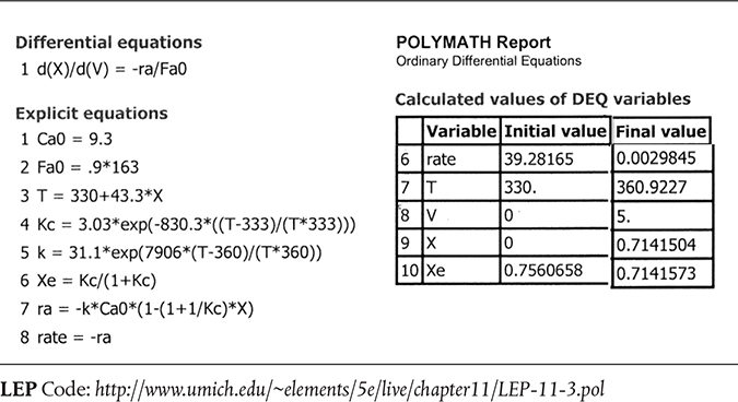
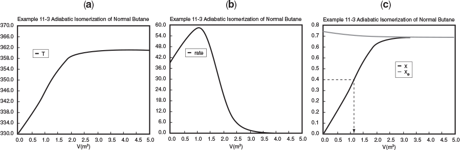
Figure E11-3.1 (a) Adiabatic PFR temperature (K), (b) Reaction rate (kmol/m³/h), and (c) conversion profiles X and X_e.

From Table 11-3.1 and Figure E11-3.1 (c) one observes that at the end of the 5 dm³ PFR both the conversion, X, and equilibrium conversion, X_e, reach 71.4%. One also notes in Figures E11-3.1 (a) and (b) that the temperature reaches a plateau of 360.9 K where the net reaction rate approaches zero at this point in the reactor. Be sure to explore each of the three parts of Figure E11-3.1 using Wolfram.

Wolfram Sliders

Analysis: Parts (a) and (b) for the PFR. The graphical output for the PFR is shown in Figure E11-3.1. We see from Figure E11-3.1(c) that a PFR volume 1.15 m³ is required for 40% conversion. The temperature and reaction-rate profiles are also shown. Notice anything strange? one observes that the rate of reaction

- r A = k C A 0      A [1 - (1 + 1 K C) X]                        B (E 11 - 3.13)

$\begin{array}{l} - r_{A} = \underset{A}{\underset{︸}{k C_{A 0}}} \underset{B}{\underset{︸}{[1 - (1 + \frac{1}{K_{C}}) X]}} & (E 11 - 3.13) \end{array}$

Look at the shape of the curves in Figure E11-3.1. Why do they look the way they do?

goes through a maximum. Near the entrance to the reactor, T increases as does k, causing term A to increase more rapidly than term B decreases, and thus the rate increases. Near the end of the reactor, term B is decreasing more rapidly than term A is increasing as we approach equilibrium. Consequently, because of these two competing effects, we have a maximum in the rate of reaction. Toward the end of the reactor, the temperature reaches a plateau as the reaction approaches equilibrium (i.e., X ≡ X_e at (V ≡ 3.5 m³)). As you know, and as do all chemical engineering students at Jofostan University in Riça, at equilibrium (–r_A ≅ 0) no further changes in X, X_e, or T take place.

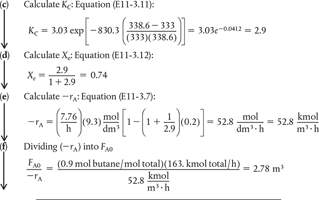
Part (c) Solution by hand calculation to perhaps give greater insight and to build on techniques in Chapter 2

We will now integrate Equation (E11-3.8) using Simpson’s rule after forming a table (E11-3.1) to calculate (F_A0/ —r_A) as a function of X. This procedure is similar to that described in Chapter 2. We now carry out a sample calculation to show how Table E11-3.1 was constructed.

For example, for X = 0.2 , follow the downward arrows for the sequence of the calculations.

We are only going to do this once!!

Sample calculation for Table E11-3.1

Continuing in this manner for other conversions, we can complete Table E11-3.2.

I know these are tedious calculations, but someone’s gotta

Cartoon shows a boy at a table sleeping over an open book with hands hanging.

TABLE E11-3.2 HAND CALCULATION

X	T(K)	k(h^-1)	K_C)	X_e)	–r_A)(kmol/m³ · h)	FA0−rA(m3) $\frac{F_{A0}}{- r_{A}} (m^{3})$
0	330	4.22	3.1	0.76	39.2	3.74
0.2	338.7	7.76	2.9	0.74	52.8	2.78
0.4	347.3	14.02	2.73	0.73	58.6	2.50
0.6	356.0	24.27	2.57	0.72	37.7	3.88
0.65	358.1	27.74	2.54	0.718	24.5	5.99
0.7	360.3	31.67	2.5	0.715	6.2	23.29

Use the data in Table E11-3.2 to make a Levenspiel plot, as in Chapter 2.

Graph shows a horizontal axis labeled X, a vertical axis labeled (F subscript (A0) over (negative r subscript A)), and an upward open parabolic curve.

(e) The reactor volume for 70% conversion will be evaluated using the quadrature formulas. Because (F_A0/–r_A) increases rapidly as we approach the adiabatic equilibrium conversion, 0.71, we will break the integral into two parts

V = \int 0.7 0 A0 - r A d X = \int 0.6 0 F A 0 - r A d X + \int 0.7 0 F A 0 - r A d X (E11-3.14)

$\begin{matrix} V = \int_{0}^{0.7} \frac{A0}{- r_{A}} d X = \int_{0}^{0.6} \frac{F_{A 0}}{- r_{A}} d X + \int_{0}^{0.7} \frac{F_{A 0}}{- r_{A}} d X & \begin{matrix} (E11-3.14) \end{matrix} \end{matrix}$

Using Equations (A-24) and (A-22) in Appendix A, we obtain

V = 3 8 \times 0.6 3 [3.74 + 3 \times 2.78 + 3 \times 2.50 + 3.88] m 3 + 1 3 \times 0.1 2 [3.88 + 4 \times 5.99 + 23.29] m 3 V = 1.75 m 3 + 0.85 m 3 V = 2.60 m 3

$\begin{array}{l} V = \frac{3}{8} \times \frac{0.6}{3} [3.74 + 3 \times 2.78 + 3 \times 2.50 + 3.88] m^{3} + \frac{1}{3} \times \frac{0.1}{2} [3.88 + 4 \times 5.99 + 23.29] m^{3} \\ V = 1.75 m^{3} + 0.85 m^{3} \\ V = 2.60 m^{3} \end{array}$

Why are we doing this hand calculation? If it isn’t helpful, send me an email and you won’t see this again.

Analysis: Part (c) You probably will never ever carry out a hand calculation similar to the one shown above. So why did we do it? Hopefully, we have given you a more intuitive feel for the magnitude of each of the terms and how they change as one moves down the reactor (i.e., what the computer solution is doing), as well as a demonstration of how the Levenspiel Plots of (F_A0/-r_A) vs. X in Chapter 2 were constructed. At the exit, V = 2.6 m³, X = 0.7, X_e = 0.715, and T = 360 K.

Later, 10/10/19: Actually, since this margin note first appeared in 2011, I have had 2 people say to keep the hand calculation in the text so I kept it in.

Is V_PFR > V_CSTR or is V_PFR < V_CSTR?

Part (d) CSTR Solution

First, take a guess. Let’s now calculate the adiabatic CSTR volume necessary to achieve 40% conversion. Do you think the CSTR will be larger or smaller than the PFR?

The CSTR mole balance is

V = F A 0 X - r A

$V = \frac{F_{A 0} X}{- r_{A}}$

Using Equation (E11-3.7) in the mole balance, we obtain

V = F A 0 X k C A 0 [ 1 - ( 1 + 1 K C ) X ] (E 11 - 3.15)

$\begin{matrix} V = \frac{F_{A 0} X}{k C_{A 0} [1 - (1 + \frac{1}{K_{C}}) X]} & (E 11 - 3.15) \end{matrix}$

From the energy balance, we have Equation (E11-3.9):

For 40% conversionT=330 + 43.4XT=330 + 43.4(0.4) = 347.3K $\begin{array}{l} For 40% conversion & \begin{array}{l} T = 330 + 43.4 X \\ T = 330 + 43.4 (0.4) = 3 47.3 K \end{array} \end{array}$

Using Equations (E11-3.10) and (E11-3.11) or from Table E11-3.1, at T = 347.3 K, we find k and K_C to be

k K C = = 14.02 h - 1 2.73

$\begin{matrix} k & = & 14.02 h^{- 1} \\ K_{C} & = & 2.73 \end{matrix}$

Then

- r A V V = = = 58.6 kmol/m 3 \cdot h ( 146.7 kmol butanc/h)(0.4) 58.6 kmol/m 3 \cdot h 1.0 m 3

$\begin{array}{l} - r_{A} & = & 58.6 {kmol/m}^{3} \cdot h \\ V & = & \frac{(146.7 kmol butanc/h)(0.4)}{58.6 {kmol/m}^{3} \cdot h} \\ V & = & 1.0 m^{3} \end{array}$

We see that the CSTR volume (1 m³) to achieve 40% conversion in this adiabatic reaction is less than the PFR volume (1.15 m³).

By recalling the Levenspiel plots from Chapter 2, we can see that the reactor volume for 40% conversion is smaller for a CSTR than for a PFR. Plotting (F_A0/ — r_A) as a function of X from the data in Table E11-3.1 is shown here.

In this example, the adiabatic CSTR volume is less than the PFR volume.

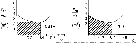
Figure Ell-3.2 Levenspiel plots for a CSTR and a PFR

The PFR area (volume) is greater than the CSTR area (volume).

Analysis: In this example we applied the CRE algorithm to a reversible-first-order reaction carried out adiabatically in a PFR and in a CSTR. We note that at the CSTR volume necessary to achieve 40% conversion is smaller than the volume to achieve the same conversion in a PFR. In Figure E11-3.1(c) we also see that at a PFR volume of about 3.5 m³, equilibrium is essentially reached about halfway through the reactor, and no further changes in temperature, reaction rate, equilibrium conversion, or conversion take place farther down the reactor.

AspenTech: Example 11-3 has also been formulated in AspenTech and can be loaded on your computer directly from the CRE Web site.

Screenshot shows buttons for Mixers/Splitters, Separators, Heat Exchangers, Columns, Reactors (selected), Pressure Changers, Manipulators, Solids, User Models, and Retired.

For reversible reactions, the equilibrium conversion, X_e, is usually calculated first.

11.5 Adiabatic Equilibrium Conversion

The highest conversion that can be achieved in reversible reactions is the equilibrium conversion. For endothermic reactions, the equilibrium conversion increases with increasing temperature up to a maximum of 1.0. For exothermic reactions, the equilibrium conversion decreases with increasing temperature.

11.5.1 Equilibrium Conversion

Exothermic Reactions. Figure 11-3(a) shows the variation of the concentration equilibrium constant, K_C as a function of temperature for an exothermic reaction (see Appendix C), and Figure 11-3(b) shows the corresponding equilibrium conversion X_e as a function of temperature. In Example 11-3, we saw that for a first-order reaction, the equilibrium conversion could be calculated using Equation (E11-3.12)

X e = K c 1 + K c (E11-3.12)

$\begin{matrix} X_{e} = \frac{K_{c}}{1 + K_{c}} & (E11-3.12) \end{matrix}$

First-order reversible reaction

Consequently, X_e can be calculated as a function of temperature directly using either Equations (E11-3.12) and (E11-3.4) or from Figure 11-3(a) and Equation (E11-3.12).

For exothermic reactions, the equilibrium conversion decreases with increasing temperature.

We note that the shape of X_e versus T curve in Figure 11-3(b) will be similar for reactions that are other than first order.

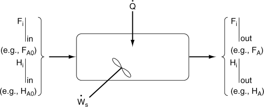
To maximum the maximum conversion that can be achieved in an exothermic reaction carried out adiabathelly, we find the intersection of the equilibrium conversion as a function of temperature (Figure 11-3(b)) with temperature-conversion relationships from the energy balance (Figure 11-2 and Equation (TII-I.A)), as shown in Figure 11-4.

X E B = Σ Θ i C P i ( T - T 0 ) - Δ H R x ( T ) (T11-1.A)

$\begin{matrix} X_{E B} = \frac{Σ Θ_{i} C_{P_{i}} (T - T_{0})}{- Δ H_{R x} (T)} & (T11-1.A) \end{matrix}$

Two graphs labeled (a) and (b) are shown.

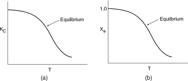
Figure 11-3 Variation of equilibrium constant and conversion with temperature for an exothermic reaction (http://www.umich.edu/~elements/5e/11chap/summary-biovan.html).

Graph shows a curve labeled Equilibrium conversion Eqn (E11-3.12).

The points T subscript 0 and T subscript 01 are marked on a horizontal axis labeled T and the points X subscript e and 1.0 are marked on the vertical axis. A curve extends horizontally from a point 1.0 on the vertical axis, slides, and extends horizontally. A straight line starts from the origin, rises from left to right, intersects the curve labeled Energy balance, and extends beyond the curve labeled Eqn (T11-1.A). A vertical arrow from the same point intersects the horizontal axis at a point labeled Adiabatic temperature and a horizontal dashed arrow intersects the vertical axis at a point labeled X subscript e. A dashed straight line starts from a point T subscript 01, rises from left to right, intersects the curve and extends beyond the curve labeled T subscript 01 is greater than T subscript 0.

Figure 11-4 Graphical solution of equilibrium and energy balance equations to obtain the adiabatic temperature and the adiabatic equilibrium conversion X_e.

Adiabatic equilibrium conversion for exothermic reactions

This intersection of the energy balance line, X_EB, with the thermodynamic equilibrium X_e curve gives the adiabatic-equilibrium conversion and temperature for an entering temperature T₀.

If the entering temperature is increased from T₀ to T₀₁, the energy balance line will be shifted to the right and be parallel to the original line, as shown by the dashed line. Note that as the inlet temperature increases, the adi-abatic equilibrium conversion decreases.

..................Content has been hidden....................

You can't read the all page of ebook, please click here login for view all page.

Table of Contents for Chapter 11 Nonisothermal Reactor Design-The Steady-State Energy Balance and Adiabatic PFR Applications

Create new playlist

Sign In

Sign Up

11. Nonisothermal Reactor Design—The Steady-State Energy Balance and Adiabatic PFR Applications

11.1 Rationale

11.2 The Energy Balance

11.2.1 First Law of Thermodynamics

11.2.2 Evaluating the Work Term

11.2.3 Overview of Energy Balances

Examples of How to Use Table 11-1.

11.3 The User-Friendly Energy Balance Equations

11.3.1 Dissecting the Steady-State Molar Flow Rates to Obtain the Heat of Reaction

11.3.2 Dissecting the Enthalpies

11.3.3 Relating ΔHRx(T), ΔH°Rx(TR), and ΔCP

11.4 Adiabatic Operation

11.4.1 Adiabatic Energy Balance

11.4.2 Adiabatic Tubular Reactor

11.5 Adiabatic Equilibrium Conversion

11.5.1 Equilibrium Conversion

Table of Contents for
Chapter 11 Nonisothermal Reactor Design-The Steady-State Energy Balance and Adiabatic PFR Applications

11.3.3 Relating ΔH_Rx(T), ΔH^°_Rx(T_R), and ΔC_P