C Analysis of Locations of Anchor Points

Search in book...
Toggle Font Controls
Create new playlist

Name your new playlist

Playlist description (optional)
Sign In

Email address

Password

Forgot Password?

or

Continue with Facebook

Continue with Google
Sign Up

Full Name

Email address

Confirm Email Address

Password

or

Continue with Facebook

Continue with Google

Appendix C
Analysis of Locations of Anchor Points

Anchor points are the optimal points in a string topology network where the addition of a long-ranged link (LL) can result in minimum average path length (APL). The identification of anchor points in a string network can serve many purposes. In Section 4.8, a detailed discussion on the significance of the anchor points can be found. Moreover, a theoretical proof of the optimal location of the first LL can be found in Section 4.8.2. Here, the estimation of the closed-form expressions of S₁, S₂, and S₃, which constitute the total path length expression in Section 4.8.2, are provided in what follows. Note that some of the previously mentioned statements are again used to make the analysis clear.

Assume that $𝒢 = (𝒱, ℰ)$ $? = (?, ℰ)$ is a string graph. Let nodes p₁ and p₂ be such that if an edge is added between p₁ and p₂, the graph APL is minimized. It can be noticed that either p₁ or p₂ would be the anchor point. Therefore, to identify the anchor points obtained by the APL optimal addition of edges to a string graph, it is sufficient to find out where a single edge should be added (i.e., to identify p₁ and p₂) to minimize the graph APL.

The nodes p₁ and p₂ are identified by considering a dense string graph. A dense string graph is of a unit diameter where infinitely large numbers of nodes are present. Formally, a dense string graph can be obtained as a limit of a sequence of string graphs, each with nodes (1, 2, . . . , N), as N → ∞. Further, assume that the distance between the nodes i and i + 1, as well as the link to be added between p₁ and p₂, is $\frac{1}{N}$ $\frac{1}{N}$ . Note that as far as optimization of APL is concerned, scaling all distances in a graph by the same quantity does not matter. The scaling which has been chosen leads to a limit graph consisting of a continuum of nodes in the interval [0, 1] (see Figure C.1(a)).

An illustration of how a dense string graph is obtained as the limit of string graphs with N nodes.

The illustration has three parts shown one below the other and labeled alphabetically. The string is represented by a long straight horizontal line, whose ends are marked 0 and 1. At about 2 centimeters to the right 0, the point p1 is marked and at about the same distance to the left of 1, the point p2 is marked. A dotted concave bi-directional arrow points to p1 and p2. Figure a shows the source s is placed between 0 and p1, almost equidistant from both points, and the destination d positioned between 1 and p2, closer to the point 1. Figure b shows s placed at about 3 centimeters to the right of p1, while d is maintained at the same position as in figure a. The distance between points s and d is spanned to be x. In figure c, the position previously marked the destination d has been marked as the source s. The dimensions of all markings are approximate.

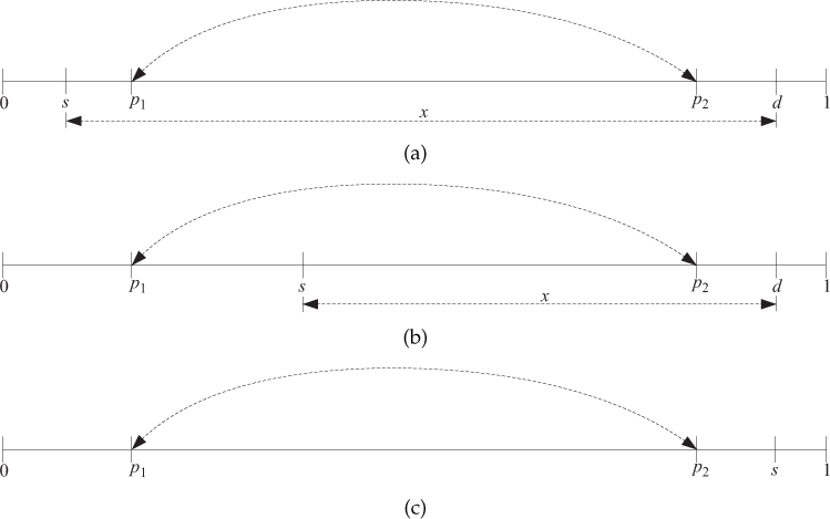
Figure C.1. A dense string graph obtained as the limit of string graphs with N nodes as N → ∞ is shown in (a). The APL is optimized with respect to the fractional positions p₁ and p₂ of the two anchor points where the first optimally added edge is connected. The shortest path length p(s, d) is different depending on whether s is in [0, p₁], (p₁, p₂), [p₂, 1]. These three cases are shown in (a), (b), and (c). In (a), s is placed at the left side of p₁ (i.e., Case 1); in (b), s is in between anchor point p₁ and anchor point p₂ (i.e., Case 2); and in (c), s is at the right side of p₂ (i.e., Case 3).

The single-edge addition problem for this limit graph can be formulated as follows. Assume that the edge is added between the positions p₁ and p₂ for the limit graph where p₁, p₂ ∈ (0, 1) and p₁ < p₂. For the limit graph in Figure C.1(a), suppose the shortest path length between nodes s and d is p (s, d). Note that p(s, d) is a function of p₁ and p₂. By a change of variables, p(s, d) can be written as p(s, x), where x = d − s. Then the total path length of all shortest paths starting from s (and considering only those d to the right of s) is $\int_{x = 0}^{1 - s} p (s, x) d x$ $\int_{x = 0}^{1 - s} p (s, x) d x$ . Then the total path length is

(C.0.1) $\int_{s = 0}^{1} \int_{x = 0}^{1 - s} p (s, x) d x d s .$ $\int_{s = 0}^{1} \int_{x = 0}^{1 - s} p (s, x) d x d s .$

Minimization of the APL for a given graph is equivalent to minimizing the total path length. Hence, the problem is to find $p_{1}^{*}$ $p_{1}^{*}$ and $p_{2}^{*}$ $p_{2}^{*}$ , optimal points for p₁ and p₂, respectively, that minimize the total path length in Equation (C.0.1).

The function p(s, x) is different depending on whether s ∈ [0, p₁], (p₁, p₂), or [p₂, 1]. Therefore, Equation (C.0.1) can be considered as the sum of three integrals, S₁, S₂, and S₃ where each term corresponding to the integral of s in [0, p₁], (p₁, p₂), or [p₂, 1] is discussed in the following.

a) Case 1: When s ∈ [0, p₁], the following subcases arise (see Figure C.1(a)):

When s + x ≤ p₁, p (s, x) = x.
When p₁ < s + x ≤ p₂, then

$\begin{matrix} p (s, x) & = & min (x, p_{1} - s + p_{2} - (s + x)) \\ = & min (x, p_{1} + p_{2} - 2 s - x) . \end{matrix}$ $\begin{matrix} p (s, x) & = & min (x, p_{1} - s + p_{2} - (s + x)) \\ = & min (x, p_{1} + p_{2} - 2 s - x) . \end{matrix}$
When p₂ < s + x

$\begin{matrix} p (s, x) & = & p_{1} - s + (s + x) - p_{2} \\ = & x + p_{1} - p_{2} . \end{matrix}$ $\begin{matrix} p (s, x) & = & p_{1} - s + (s + x) - p_{2} \\ = & x + p_{1} - p_{2} . \end{matrix}$

Then it can be seen that

(C.0.2) $S_{1} = \int_{0}^{p_{1}} \int_{0}^{1 - s} p (s, x) d x d s,$ $S_{1} = \int_{0}^{p_{1}} \int_{0}^{1 - s} p (s, x) d x d s,$

where $\int_{0}^{1 - s} p (s, x) d x$ $\int_{0}^{1 - s} p (s, x) d x$ is

$\begin{matrix} \int_{0}^{p_{1} - s} x d x + \int_{p_{1} - s}^{\frac{p_{1} + p_{2}}{2} - s} x d x + \\ \int_{\frac{p_{1} + p_{2}}{2} - s}^{p_{2} - s} (p_{1} + p_{2} - 2 s - x) d x + \int_{p_{2} - s}^{1 - s} (x + p_{1} - p_{2}) d x . \end{matrix}$ $\begin{matrix} \int_{0}^{p_{1} - s} x d x + \int_{p_{1} - s}^{\frac{p_{1} + p_{2}}{2} - s} x d x + \\ \int_{\frac{p_{1} + p_{2}}{2} - s}^{p_{2} - s} (p_{1} + p_{2} - 2 s - x) d x + \int_{p_{2} - s}^{1 - s} (x + p_{1} - p_{2}) d x . \end{matrix}$

b) Case 2: When s ∈ (p₁, p₂), there are two possibilities (see Figure C.1(b)) for the shortest path p (s, x):

When s + x ≤ p₂,

$\begin{matrix} p (s, x) & = & min (x, s - p_{1} + p_{2} - (s + x)) \\ = & min (x, p_{2} - p_{1} - x) . \end{matrix}$ $\begin{matrix} p (s, x) & = & min (x, s - p_{1} + p_{2} - (s + x)) \\ = & min (x, p_{2} - p_{1} - x) . \end{matrix}$
When s + x > p₂,

$\begin{matrix} p (s, x) & = & min (x, s - p_{1} + (s + x) - p_{2}) \\ = & min (x, 2 s + x - p_{1} - p_{2}) . \end{matrix}$ $\begin{matrix} p (s, x) & = & min (x, s - p_{1} + (s + x) - p_{2}) \\ = & min (x, 2 s + x - p_{1} - p_{2}) . \end{matrix}$

Similarly, using Equation (C.0.1), S₂ is obtained as

(C.0.3) $\begin{matrix} \int_{p_{1}}^{p_{2}} \int_{0}^{1 - s} p (s, x) d x d s = \\ \int_{p_{1}}^{\frac{p_{1} + p_{2}}{2}} Y d s + \int_{\frac{p_{1} + p_{2}}{2}}^{p_{2}} \int_{0}^{p_{2} - s} x d x d s + \int_{\frac{p_{1} + p_{2}}{2}}^{p_{2}} \int_{p_{2} - s}^{1 - s} x d x d s, \end{matrix}$ $\begin{matrix} \int_{p_{1}}^{p_{2}} \int_{0}^{1 - s} p (s, x) d x d s = \\ \int_{p_{1}}^{\frac{p_{1} + p_{2}}{2}} Y d s + \int_{\frac{p_{1} + p_{2}}{2}}^{p_{2}} \int_{0}^{p_{2} - s} x d x d s + \int_{\frac{p_{1} + p_{2}}{2}}^{p_{2}} \int_{p_{2} - s}^{1 - s} x d x d s, \end{matrix}$

where $Y = \int_{0}^{\frac{p_{2} - p_{1}}{2}} x d x + \int_{\frac{p_{2} - p_{1}}{2}}^{p_{2} - s} (p_{2} - p_{1} - x) d x .$ $Y = \int_{0}^{\frac{p_{2} - p_{1}}{2}} x d x + \int_{\frac{p_{2} - p_{1}}{2}}^{p_{2} - s} (p_{2} - p_{1} - x) d x .$

c) Case 3: When s ∈ [p₂, 1] (see Figure C.1(c)), from Equation (C.0.1) it can be obtained that

(C.0.4) $S_{3} = \int_{p_{2}}^{1} \int_{0}^{1 - s} x d x d s .$ $S_{3} = \int_{p_{2}}^{1} \int_{0}^{1 - s} x d x d s .$

Combining Equation (C.0.2), Equation (C.0.3), and Equation (C.0.4), the following observations can be made:

(C.0.5) $\begin{matrix} \int_{s = 0}^{1} \int_{x = 0}^{1 - s} p (s, x) d x d s & = & S_{1} + S_{2} + S_{3} \\ P (f_{1}, f_{2}) & = & \frac{5}{24} (p_{2}^{3} - p_{1}^{3}) - \frac{1}{4} (p_{2}^{2} - 3 p_{1}^{2}) + \\ \frac{3}{8} p_{1} p_{2} (p_{2} - p_{1} - \frac{4}{3}) + \frac{1}{6} . \end{matrix}$ $\begin{matrix} \int_{s = 0}^{1} \int_{x = 0}^{1 - s} p (s, x) d x d s & = & S_{1} + S_{2} + S_{3} \\ P (f_{1}, f_{2}) & = & \frac{5}{24} (p_{2}^{3} - p_{1}^{3}) - \frac{1}{4} (p_{2}^{2} - 3 p_{1}^{2}) + \\ \frac{3}{8} p_{1} p_{2} (p_{2} - p_{1} - \frac{4}{3}) + \frac{1}{6} . \end{matrix}$

Therefore, our problem is to

(C.0.6) $\begin{matrix} minimize & P (p_{1}, p_{2}) \\ such that & p_{1}, p_{2} \in (0, 1), \\ p_{1} < p_{2} . \end{matrix}$ $\begin{matrix} minimize & P (p_{1}, p_{2}) \\ such that & p_{1}, p_{2} \in (0, 1), \\ p_{1} < p_{2} . \end{matrix}$

Note that P(p₁, p₂) is a strictly convex function (Hessian with respect to p₁ and p₂ can be shown to be positive definite) in the constraint set and can be solved in constant time.

The optimal values of p₁ and p₂—that is, $p_{1}^{*}$ $p_{1}^{*}$ and $p_{2}^{*}$ $p_{2}^{*}$ , respectively—can be obtained from Equation (C.0.6), as 0.2071 and 0.7929, which are unique. Figure C.2 shows a 2-D contour plot of the objective function P(p₁, p₂). From the analytical derivation, therefore, it can be seen that the fractional positions of the anchor points for a dense string topology network coincide with the observation in [74].

A graph illustrating the objective function P(p1, p2) with the constraint that p1 is lesser than p2.

Figure C.2. Objective function P(p₁, p₂) in the constraint set p₁ < p₂. © [2016] IEEE. Reprinted, with permission, from A. Chakraborty, Vineeth B. S., and B. S. Manoj, “Analytical identification of anchor nodes in a small-world network,” in IEEE Communications Letters, vol. 20, no. 6, pp. 1215–1218, June 2016.

..................Content has been hidden....................

You can't read the all page of ebook, please click here login for view all page.

Table of Contents for C Analysis of Locations of Anchor Points

Create new playlist

Sign In

Sign Up

Appendix CAnalysis of Locations of Anchor Points

Table of Contents for
C Analysis of Locations of Anchor Points

Appendix C
Analysis of Locations of Anchor Points