
9
Compression
9.1 Introduction to compression
Compression, bit rate reduction and data reduction are all terms which mean basically the same thing in this context. In essence the same (or nearly the same) information is carried using a smaller quantity or rate of data. It should be pointed out that, in audio, compression traditionally means a process in which the dynamic range of the sound is reduced. Provided the context is clear, the two meanings can co-exist without a great deal of confusion.
There are several reasons why compression techniques are popular:
(a)Compression extends the playing time of storage devices such as file servers.
(b)Compression allows miniaturization. With less data to store, the same playing time is obtained with smaller hardware. This is the approach used in the DV video tape format, DVD and MiniDisc.
(c)Tolerances can be relaxed. With less data to record, storage density can be reduced making equipment which is more resistant to adverse environments and which requires less maintenance.
(d)In communication systems, compression allows a reduction in bandwidth, hence the use in digital television broadcasting. Where the communication is billed by the bit, compression will result in a reduction in cost. Compression may also make possible some process which would be impracticable without it, such as Internet video.
(e)If a given bandwidth is available to an uncompressed signal, compression allows faster than real-time transmission in the same bandwidth.
(f)If a given bandwidth is available, compression allows a better-quality signal in the same bandwidth.
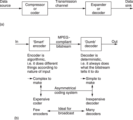
Compression is summarized in Figure 9.1. It will be seen in (a) that the data rate is reduced at source by the compressor. The compressed data are then passed through a communication channel and returned to the original rate by the expander. The ratio between the source data rate and the channel data rate is called the compression factor. The term coding gain is also used. Sometimes a compressor and expander in series are referred to as a compander. The compressor may equally well be referred to as a coder and the expander a decoder in which case the tandem pair may be called a codec.
In audio and video compression, where the encoder is more complex than the decoder the system is said to be asymmetrical as in Figure 9.1(b). The encoder needs to be algorithmic or adaptive whereas the decoder is ‘dumb’ and carries out fixed actions. This is advantageous in applications such as broadcasting where the number of expensive complex encoders is small but the number of simple inexpensive decoders is large. In point-topoint applications or in recorders the advantage of asymmetrical coding is not so great.
Although there are many different coding techniques, all of them fall into one or other of these categories. In lossless coding, the data from the expander are identical bit-for-bit with the original source data. The socalled ‘stacker’ programs which increase the apparent capacity of disk drives in personal computers use lossless codecs. Clearly with computer programs the corruption of a single bit can be catastrophic. Lossless coding is generally restricted to compression factors of around 2:1.
It is important to appreciate that a lossless coder cannot guarantee a particular compression factor and the communications link or recorder used with it must be able to function with the variable output data rate. Source data which result in poor compression factors on a given codec are described as difficult. It should be pointed out that the difficulty is often a function of the codec. In other words data which one codec finds difficult may not be found difficult by another. Lossless codecs can be included in bit-error-rate testing schemes. It is also possible to cascade or concatenate lossless codecs without any special precautions.
In lossy coding, data from the expander are not identical bit-for-bit with the source data and as a result comparing the input with the output is bound to reveal differences. Lossy codecs are not suitable for computer data, but are used in audio and video as they allow greater compression factors than lossless codecs. Successful lossy codecs are those in which the errors are arranged so that a human viewer or listener finds them subjectively difficult to detect. Thus lossy codecs must be based on an understanding of psychoacoustic and psychovisual perception and are often called perceptive codes.
In perceptive coding, the greater the compression factor required, the more accurately must the human senses be modelled. Perceptive coders can be forced to operate at a fixed compression factor. This is convenient for practical transmission applications where a fixed data rate is easier to handle than a variable rate. The result of a fixed compression factor is that the subjective quality can vary with the ‘difficulty’ of the input material. Perceptive codecs should not be concatenated indiscriminately especially if they use different algorithms. As the reconstructed signal from a perceptive codec is not bit-for-bit accurate, clearly such a codec cannot be included in any bit error rate testing system as the coding differences would be indistinguishable from real errors.
Although the adoption of digital techniques to images is recent, compression itself is as old as television. Figure 9.2 shows some of the compression techniques used in traditional television systems.
One of the oldest techniques is interlace which has been used in analog television from the very beginning as a primitive way of reducing bandwidth. As was seen in Chapter 7, interlace is not without its problems, particularly in motion rendering. MPEG supports interlace simply because legacy interlaced signals exist and there is a requirement to compress them. This should not be taken to mean that it is a good idea.
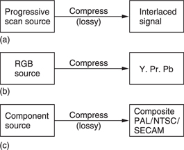
The generation of colour difference signals from RGB in video represents an application of perceptive coding. The human visual system (HVS) sees no change in quality although the bandwidth of the colour difference signals is reduced. This is because human perception of detail in colour changes is much less than in brightness changes. This approach is sensibly retained in MPEG.
Composite video systems such as PAL, NTSC and SECAM are all analog compression schemes which embed a subcarrier in the luminance signal so that colour pictures are available in the same bandwidth as monochrome. In comparison with a progressive scan RGB picture, interlaced composite video has a compression factor of 6:1.
In a sense MPEG can be considered to be a modern digital equivalent of analog composite video as it has most of the same attributes. For example, the eight-field sequence of a PAL subcarrier which makes editing diffficult has its equivalent in the GOP (group of pictures) of MPEG.1
In a PCM digital system the bit rate is the product of the sampling rate and the number of bits in each sample and this is generally constant. Nevertheless the information rate of a real signal varies. In all real signals, part of the signal is obvious from what has gone before or what may come later and a suitable receiver can predict that part so that only the true information actually has to be sent. If the characteristics of a predicting receiver are known, the transmitter can omit parts of the message in the knowledge that the receiver has the ability to re-create it. Thus all encoders must contain a model of the decoder.
One definition of information is that it is the unpredictable or surprising element of data. Newspapers are a good example of information because they only mention items which are surprising. Newspapers never carry items about individuals who have not been involved in an accident as this is the normal case. Consequently the phrase ‘no news is good news’ is remarkably true because if an information channel exists but nothing has been sent then it is most likely that nothing remarkable has happened.
The difference between the information rate and the overall bit rate is known as the redundancy. Compression systems are designed to eliminate as much of that redundancy as practicable or perhaps affordable. One way in which this can be done is to exploit statistical predictability in signals. The information content or entropy of a sample is a function of how different it is from the predicted value. Most signals have some degree of predictability. A sine wave is highly predictable, because all cycles look the same. According to Shannon's theory, any signal which is totally predictable carries no information. In the case of the sine wave this is clear because it represents a single frequency and so has no bandwidth.
At the opposite extreme a signal such as noise is completely unpredictable and as a result all codecs find noise difficult. There are two consequences of this characteristic. First, a codec which is designed using the statistics of real material should not be tested with random noise because it is not a representative test. Second, a codec which performs well with clean source material may perform badly with source material containing superimposed noise. Most practical compression units require some form of preprocessing before the compression stage proper and appropriate noise reduction should be incorporated into the preprocessing if noisy signals are anticipated. It will also be necessary to restrict the degree of compression applied to noisy signals.
All real signals fall part-way between the extremes of total predictability and total unpredictability or noisiness. If the bandwidth (set by the sampling rate) and the dynamic range (set by the wordlength) of the transmission system are used to delineate an area, this sets a limit on the information capacity of the system. Figure 9.3(a) shows that most real signals occupy only part of that area. The signal may not contain all frequencies, or it may not have full dynamics at certain frequencies.
Entropy can be thought of as a measure of the actual area occupied by the signal. This is the area that must be transmitted if there are to be no subjective differences or artifacts in the received signal. The remaining area is called the redundancy because it adds nothing to the information conveyed. Thus an ideal coder could be imagined which miraculously sorts out the entropy from the redundancy and sends only the former. An ideal decoder would then re-create the original impression of the information quite perfectly.
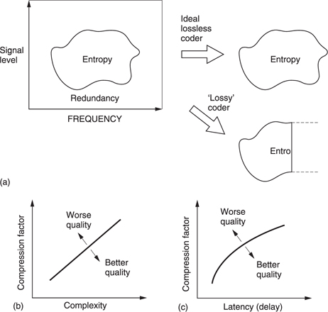
Figure 9.3 (a) A perfect coder removes only the redundancy from the input signal and results in subjectively lossless coding. If the remaining entropy is beyond the capacity of the channel some of it must be lost and the codec will then be lossy. An imperfect coder will also be lossy as it fails to keep all entropy. (b) As the compression factor rises, the complexity must also rise to maintain quality. (c) High compression factors also tend to increase latency or delay through the system.
As the ideal is approached, the coder complexity and the latency or delay both rise. Figure 9.3(b) shows how complexity increases with compression factor. This can be seen in the relative complexities of MPEG-1, 2 and 4. Figure 9.3(c) shows how increasing the codec latency can improve the compression factor. Obviously we would have to provide a channel which could accept whatever entropy the coder extracts in order to have transparent quality. As a result moderate coding gains which only remove redundancy need not cause artifacts and result in systems which are described as subjectively lossless.
If the channel capacity is not sufficient for that, then the coder will have to discard some of the entropy and with it useful information. Larger coding gains which remove some of the entropy must result in artifacts. It will also be seen from Figure 9.3 that an imperfect coder will fail to separate the redundancy and may discard entropy instead, resulting in artifacts at a suboptimal compression factor.
A single variable-rate transmission or recording channel is inconvenient and unpopular with channel providers because it is difficult to police. The requirement can be overcome by combining several compressed channels into one constant rate transmission in a way which flexibly allocates data rate between the channels. Provided the material is unrelated, the probability of all channels reaching peak entropy at once is very small and so those channels which are at one instant passing easy material will free up transmission capacity for those channels which are handling difficult material. This is the principle of statistical multiplexing.
Where the same type of source material is used consistently, e.g. English text, then it is possible to perform a statistical analysis on the frequency with which particular letters are utilized. Variable-length coding is used in which frequently used letters are allocated short codes and letters which occur infrequently are allocated long codes. This results in a lossless code. The well-known Morse code used for telegraphy is an example of this approach. The letter e is the most frequent in English and is sent with a single dot. An infrequent letter such as z is allocated a long complex pattern. It should be clear that codes of this kind which rely on a prior knowledge of the statistics of the signal are only effective with signals actually having those statistics. If Morse code is used with another language, the transmission becomes significantly less efficient because the statistics are quite different; the letter z, for example, is quite common in Czech.
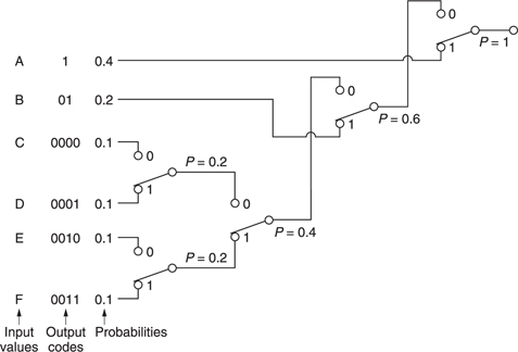
The Huffman code2 is one which is designed for use with a data source having known statistics and shares the same principles with the Morse code. The probability of the different code values to be transmitted is studied, and the most frequent codes are arranged to be transmitted with short wordlength symbols. As the probability of a code value falls, it will be allocated longer wordlength. The Huffman code is used in conjunction with a number of compression techniques and is shown in Figure 9.4.
The input or source codes are assembled in order of descending probability. The two lowest probabilities are distinguished by a single code bit and their probabilities are combined. The process of combining probabilities is continued until unity is reached and at each stage a bit is used to distinguish the path. The bit will be a zero for the most probable path and one for the least. The compressed output is obtained by reading the bits which describe which path to take going from right to left.
In the case of computer data, there is no control over the data statistics. Data to be recorded could be instructions, images, tables, text files and so on; each having their own code value distributions. In this case a coder relying on fixed source statistics will be completely inadequate. Instead a system is used which can learn the statistics as it goes along. The Lempel—Ziv-Welch (LZW) lossless codes are in this category. These codes build up a conversion table between frequent long source data strings and short transmitted data codes at both coder and decoder and initially their compression factor is below unity as the contents of the conversion tables are transmitted along with the data. However, once the tables are established, the coding gain more than compensates for the initial loss. In some applications, a continuous analysis of the frequency of code selection is made and if a data string in the table is no longer being used with sufficient frequency it can be deselected and a more common string substituted.
Lossless codes are less common for audio and video coding where perceptive codes are permissible. The perceptive codes often obtain a coding gain by shortening the wordlength of the data representing the signal waveform. This must increase the noise level and the trick is to ensure that the resultant noise is placed at frequencies where human senses are least able to perceive it. As a result although the received signal is measureably different from the source data, it can appear the same to the human listener or viewer at moderate compression factors. As these codes rely on the characteristics of human sight and hearing, they can only be fully tested subjectively.
The compression factor of such codes can be set at will by choosing the wordlength of the compressed data. Whilst mild compression will be undetectable, with greater compression factors, artifacts become noticeable. Figure 9.3 shows that this is inevitable from entropy considerations.
9.2 Compression standards
Standards are important in compression because without a suitable decoder, compressed data are meaningless. The MPEG standards are possibly the most well known, but they are certainly not the only standards. In video recording, the DV standard is also important. There are also a number of obsolescent standards which predated MPEG, and various proprietary schemes.
MPEG is actually an acronym for the Moving Pictures Experts Group which was formed by the ISO (International Standards Organization) to set standards for audio and video compression and transmission. The first compression standard for audio and video was MPEG-1.3,4 MPEG-1 was initially designed to allow pictures and sound to be carried in the standard bit rate of a Compact Disc. Achieving such a low bit rate at the time required considerable spatial and temporal subsampling of standard definition television down to what is known as SIF (source intermediate format). Figure 9.5 shows that SIF discards every other field in the input to halve the picture rate and eliminate interlace. Discarding alternate picture lines in this way halves vertical resolution and the horizontal resolution is also halved to match. Chroma data are further downsampled. MPEG-1 was of limited quality and application and the subsequent MPEG-2 standard was considerably broader in scope and of wider appeal. For example, MPEG-2 supports interlace and a much wider range of picture sizes and bit rates. The MPEG-4 standard uses the tools of MPEG-2 but adds to them to allow even higher compression factors. MPEG standards are largely backward compatible such that an MPEG-2 decoder can understand MPEG-1 data and an MPEG-4 decoder can understand both MPEG-2 and MPEG-1 data.
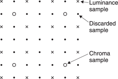
Figure 9.5 In MPEG-1, the input format is known as SIF (source intermediate format) and is created from interlaced video by discarding alternate fields and downsampling those that remain
The approach of the ISO to standardization in MPEG is novel because it is not the encoder which is standardized. Figure 9.6(a) shows that instead the way in which a decoder shall interpret the bitstream is defined. A decoder which can successfully interpret the bitstream is said to be compliant. Figure 9.6(b) shows that the advantage of standardizing the decoder is that over time encoding algorithms can improve yet compliant decoders will continue to function with them.
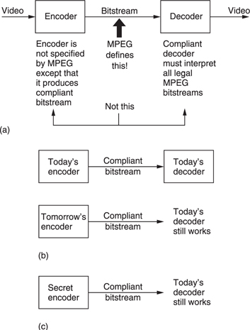
Figure 9.6 (a) MPEG defines the protocol of the bitstream between encoder and decoder. The decoder is defined by implication, the encoder is left very much to the designer. (b) This approach allows future encoders of better performance to remain compatible with existing decoders. (c) This approach also allows an encoder to produce a standard bitstream while its technical operation remains a commercial secret.
Manufacturers can supply encoders using algorithms which are proprietary and their details do not need to be published. A useful result is that there can be competition between different encoder designs which means that better designs will evolve. The user will have greater choice because different levels of cost and complexity can exist in a range of coders yet a compliant decoder will operate with them all.
MPEG is, however, much more than a compression scheme as it also standardizes the protocol and syntax under which it is possible to combine or multiplex audio data with video data to produce a digital equivalent of a television program. Many such programs can be combined in a single multiplex and MPEG defines the way in which such multiplexes can be created and transported. The definitions include the metadata which decoders require to demultiplex correctly and which users will need to locate programs of interest. As with all video systems there is a requirement for synchronizing or genlocking and this is particularly complex when a multiplex is assembled from many signals which are not necessarily synchronized to one another
The applications of audio and video compression are limitless and the ISO has done well to provide standards which are appropriate to the wide range of possible compression products.
MPEG embraces video pictures from the tiny screen of a videophone to the high-definition images needed for electronic cinema. Audio coding stretches from speech-grade mono to multichannel surround sound.
Figure 9.7 shows the use of a codec with a recorder. The playing time of the medium is extended in proportion to the compression factor. In the case of tapes, the access time is improved because the length of tape needed for a given recording is reduced and so it can be rewound more quickly.
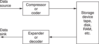
Figure 9.7 Compression can be used around a recording medium. The storage capacity may be increased or the access time reduced according to the application.
In the case of DVD (digital video disk, aka digital versatile disk) the challenge was to store an entire movie on one 12 cm disk. The storage density available with today's optical disk technology is such that recording of conventional uncompressed video would be out of the question.
In communications, the cost of data links is often roughly proportional to the data rate and so there is simple economic pressure to use a high compression factor. However, it should be borne in mind that implementing the codec also has a cost which rises with compression factor and so a degree of compromise will be inevitable. It should also be appreciated that the cost of communications is a moving target. The adoption of optical fibres has made bandwidth essentially limitless between major centres, leaving the bandwidth issue primarily in the so-called ‘last mile’ from such centres to the home. In the case of Video-On-Demand, technology such as ADSL (see Chapter 12) exists to convey data to the home on existing copper telephone lines, but the available bit rate is insufficient for entertainment-grade video without compression.
In workstations designed for the editing of audio and/or video, the source material is stored on hard disks for rapid access. Whilst top-grade systems may function without compression, many systems use compression to offset the high cost of disk storage. When a workstation is used for off-line editing, a high compression factor can be used and artifacts will be visible in the picture.
This is of no consequence as the picture is only seen by the editor who uses it to make an EDL (edit decision list) which is no more than a list of actions and the timecodes at which they occur. The original uncompressed material is then conformed to the EDL to obtain high-quality edited work. When on-line editing is being performed, the output of the workstation is the finished product and clearly a lower compression factor will have to be used.
Perhaps it is in broadcasting where the use of compression will have its greatest impact. There is only one electromagnetic spectrum and pressure from other services such as cellular telephones makes efficient use of bandwidth mandatory. Analog television broadcasting is an old technology and makes very inefficient use of bandwidth. Its replacement by a compressed digital transmission will be inevitable for the practical reason that the bandwidth is needed elsewhere.
Fortunately in broadcasting there is a mass market for decoders and these can be implemented as low-cost integrated circuits. Fewer encoders are needed and so it is less important if these are expensive. Whilst the cost of digital storage goes down year on year, the cost of electromagnetic spectrum goes up. Consequently in the future the pressure to use compression in recording will ease whereas the pressure to use it in radio communications will increase.
9.3 Profiles, levels and layers
MPEG-2 has too many applications to solve with a single standard and so it is subdivided into Profiles and Levels. Put simply a Profile describes a degree of complexity whereas a Level describes the picture size or resolution which goes with that Profile. Not all Levels are supported at all Profiles. Figure 9.8 shows the available combinations. In principle there are 24 of these, but not all have been defined. An MPEG decoder having a given Profile and Level must also be able to decode lower profiles and levels.
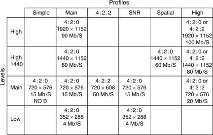
The simple profile does not support bidirectional coding and so only I and P pictures will be output. This reduces the coding and decoding delay and allows simpler hardware. The simple profile has only been defined at Main level (SP@ML).
The Main Profile is designed for a large proportion of uses. The low level uses a low-resolution input having only 352 pixels per line. The majority of broadcast applications will require the MP@ML (Main Profile at Main Level) subset of MPEG which supports SDTV (standard definition television).
The High-1440 level is a high-definition scheme which doubles the definition compared to main level. The high level not only doubles the resolution but maintains that resolution with 16:9 format by increasing the number of horizontal samples from 1440 to 1920.
In compression systems using spatial transforms and requantizing it is possible to produce scaleable signals. A scaleable process is one in which the input results in a main signal and a ‘helper’ signal. The main signal can be decoded alone to give a picture of a certain quality, but if the information from the helper signal is added some aspect of the quality can be improved.
Figure 9.9(a) shows that in a conventional MPEG coder, by heavily requantizing coefficients a picture with moderate signal-to-noise ratio results. If, however, that picture is locally decoded and subtracted pixel by pixel from the original, a ‘quantizing noise’ picture would result. This can be compressed and transmitted as the helper signal. A simple decoder decodes only the main ‘noisy’ bitstream, but a more complex decoder can decode both bitstreams and combine them to produce a lownoise picture. This is the principle of SNR scaleability.

As an alternative, Figure 9.9(b) shows that by coding only the lower spatial frequencies in a HDTV picture a main bitstream can be made which an SDTV receiver can decode. If the lower-definition picture is locally decoded and subtracted from the original picture, a ‘definitionenhancing’ picture would result. This can be coded into a helper signal. A suitable decoder could combine the main and helper signals to re-create the HDTV picture. This is the principle of spatial scaleability.
The High profile supports both SNR and spatial scaleability as well as allowing the option of 4:2:2 sampling (see section 7.14).
The 4:2:2 profile has been developed for improved compatibility with existing digital television production equipment. This allows 4:2:2 working without requiring the additional complexity of using the high profile. For example, a HP@ML decoder must support SNR scaleability which is not a requirement for production.
In MPEG audio the different requirements are met using layers. Layer I is the least complex, but gives the lowest compression factor, Layer II is more complex, but maintains quality at lower bit rates, whereas Layer III is extremely complex and is optimized for very high compression factors. Subsequently MPEG-AAC (advanced audio coding) was developed which allows better audio quality through increased complexity. However, AAC is not compatible with the earlier systems.
9.4 Spatial and temporal redundancy in MPEG
Video signals exist in four dimensions: these are the attributes of the sample, the horizontal and vertical spatial axes and the time axis. Compression can be applied in any or all of those four dimensions. MPEG assumes eight-bit colour difference signal as the input, requiring rounding if the source is ten-bit. The sampling rate of the colour signals is less than that of the luminance. This is done by downsampling the colour samples horizontally and generally vertically as well. Essentially an MPEG system has three parallel simultaneous channels, one for luminance and two colour difference, which after coding are multiplexed into a single bitstream.
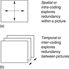
Figure 9.10 (a) Spatial or intra-coding works on individual images. (b) Temporal or inter-coding works on successive images.
Figure 9.10(a) shows that when individual pictures are compressed without reference to any other pictures, the time axis does not enter the process which is therefore described as intra-coded (intra = within) compression. The term spatial coding will also be found. It is an advantage of intra-coded video that there is no restriction to the editing which can be carried out on the picture sequence. As a result compressed VTRs intended for production use spatial coding. Cut editing may take place on the compressed data directly if necessary. As spatial coding treats each picture independently, it can employ certain techniques developed for the compression of still pictures. The ISO JPEG (Joint Photographic Experts Group) compression standards5,6 are in this category. Where a succession of JPEG coded images are used for television, the term ‘Motion JPEG’ will be found.
Greater compression factors can be obtained by taking account of the redundancy from one picture to the next. This involves the time axis, as Figure 9.10(b) shows, and the process is known as inter-coded (inter = between) or temporal compression.
Temporal coding allows a higher compression factor, but has the disadvantage that an individual picture may exist only in terms of the differences from a previous picture. Clearly editing must be undertaken with caution and arbitrary cuts simply cannot be performed on the MPEG bitstream. If a previous picture is removed by an edit, the difference data will then be insufficient to re-create the current picture.
Intra-coding works in three dimensions on the horizontal and vertical spatial axes and on the sample values. Analysis of typical television pictures reveals that whilst there is a high spatial frequency content due to detailed areas of the picture, there is a relatively small amount of energy at such frequencies. Often pictures contain sizeable areas in which the same or similar pixel values exist. This gives rise to low spatial frequencies. The average brightness of the picture results in a substantial zero frequency component. Simply omitting the high-frequency components is unacceptable as this causes an obvious softening of the picture.
A coding gain can be obtained by taking advantage of the fact that the amplitude of the spatial components falls with frequency. It is also possible to take advantage of the eye's reduced sensitivity to noise in high spatial frequencies. If the spatial frequency spectrum is divided into frequency bands the high-frequency bands can be described by fewer bits not only because their amplitudes are smaller but also because more noise can be tolerated. The wavelet transform and the discrete cosine transfrm used in MPEG allow two-dimensional pictures to be described in the frequency domain. These were discussed in Chapter 3.
Inter-coding takes further advantage of the similarities between successive pictures in real material. Instead of sending information for each picture separately, inter-coders will send the difference between the previous picture and the current picture in a form of differential coding. Figure 9.11 shows the principle. A picture store is required at the coder to allow comparison to be made between successive pictures and a similar store is required at the decoder to make the previous picture available. The difference data may be treated as a picture itself and subjected to some form of transform-based spatial compression.
The simple system of Figure 9.11(a) is of limited use as in the case of a transmission error, every subsequent picture would be affected. Channel switching in a television set would also be impossible. In practical systems a modification is required. One approach is the so-called ‘leaky predictor’ in which the next picture is predicted from a limited number of previous pictures rather than from an indefinite number. As a result errors cannot propagate indefinitely. The approach used in MPEG is that periodically some absolute picture data are transmitted in place of difference data.
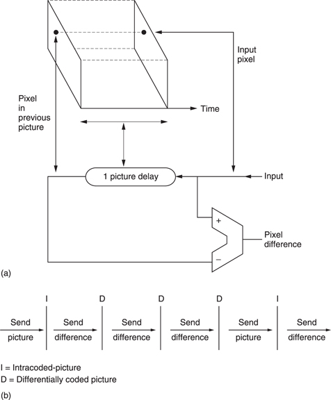
Figure 9.11(b) shows that absolute picture data, known as I or intra pictures are interleaved with pictures which are created using difference data, known as P or predicted pictures. The I pictures require a large amount of data, whereas the P pictures require less data. As a result the instantaneous data rate varies dramatically and buffering has to be used to allow a constant transmission rate. The leaky predictor needs less buffering as the compression factor does not change so much from picture to picture.
The I picture and all the P pictures prior to the next I picture are called a group of pictures (GOP). For a high compression factor, a large number of P pictures should be present between I pictures, making a long GOP. However, a long GOP delays recovery from a transmission error. The compressed bitstream can only be edited at I pictures as shown.
In the case of moving objects, although their appearance may not change greatly from picture to picture, the data representing them on a fixed sampling grid will change and so large differences will be generated between successive pictures. It is a great advantage if the effect of motion can be removed from difference data so that they reflect only the changes in appearance of a moving object since a much greater coding gain can then be obtained. This is the objective of motion compensation.
In real television program material objects move around before a fixed camera or the camera itself moves. Motion compensation is a process which effectively measures motion of objects from one picture to the next so that it can allow for that motion when looking for redundancy between pictures. Chapter 7 showed that moving pictures can be expressed in a three-dimensional space which results from the screen area moving along the time axis. In the case of still objects, the only motion is along the time axis. However, when an object moves, it does so along the optic flow axis which is not parallel to the time axis. The optic flow axis joins the same point on a moving object as it takes on various screen positions.
It will be clear that the data values representing a moving object change with respect to the time axis. However, looking along the optic flow axis the appearance of an object changes only if it deforms, moves into shadow or rotates. For simple translational motions the data representing an object are highly redundant with respect to the optic flow axis. Thus if the optic flow axis can be located, coding gain can be obtained in the presence of motion.
A motion-compensated coder works as follows. An I picture is sent, but is also locally stored so that it can be compared with the next input picture to find motion vectors for various areas of the picture. The I picture is then shifted according to these vectors to cancel inter-picture motion. The resultant predicted picture is compared with the actual picture to produce a prediction error also called a residual. The prediction error is transmitted with the motion vectors. At the receiver the original I picture is also held in a memory. It is shifted according to the transmitted motion vectors to create the predicted picture and then the prediction error is added to it to re-create the original. When a picture is encoded in this way MPEG calls it a P picture.
The concept of sending a prediction error is a useful approach because it allows both the motion estimation and compensation to be imperfect.
A good motion-compensation system will send just the right amount of vector data. With insufficient vector data, the prediction error will be large, but transmission of excess vector data will also cause the the bit rate to rise. There will be an optimum balance which minimizes the sum of the prediction error data and the vector data.
In MPEG-2 the balance is obtained by dividing the screen into areas called macroblocks which are 16 luminance pixels square. Each macroblock is steered by a vector. The location of the boundaries of a macroblock are fixed and so the vector does not move the macroblock. Instead the vector tells the decoder where to look in another frame to find pixel data to fetch to the macroblock. Figure 9.12(a) shows this concept. The shifting process is generally done by modifying the read address of a RAM using the vector. This can shift by one pixel steps. MPEG-2 vectors have half-pixel resolution so it is necessary to interpolate between pixels from RAM to obtain half-pixel shifted values.
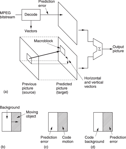
Figure 9.12 (a) In motion compensation, pixel data are brought to a fixed macroblock in the target picture from a variety of places in another picture. (b) Where only part of a macroblock is moving, motion compensation is non-ideal. The motion can be coded (c), causing a prediction error in the background, or the background can be coded (d) causing a prediction error in the moving object.
Real moving objects will not coincide with macroblocks and so the motion compensation will not be ideal but the prediction error makes up for any shortcomings. Figure 9.12(b) shows the case where the boundary of a moving object bisects a macroblock. If the system measures the moving part of the macroblock and sends a vector, the decoder will shift the entire block making the stationary part wrong. If no vector is sent, the moving part will be wrong. Both approaches are legal in MPEG-2 because the prediction error sorts out the incorrect values. An intelligent coder might try both approaches to see which required the least prediction error data.
The prediction error concept also allows the use of simple but inaccurate motion estimators in low-cost systems. The greater prediction error data are handled using a higher bit rate. On the other hand, if a precision motion estimator is available, a very high compression factor may be achieved because the prediction error data are minimized. MPEG-2 does not specify how motion is to be measured; it simply defines how a decoder will interpret the vectors. Encoder designers are free to use any motionestimation system provided that the right vector protocol is created. Chapter 3 contrasted a number of motion-estimation techniques.
Figure 9.13(a) shows that a macroblock contains both luminance and colour difference data at different resolutions. Most of the MPEG-2 Profiles use a 4:2:0 structure which means that the colour is downsampled by a factor of two in both axes. Thus in a 16 × 16 pixel block, there are only 8 × 8 colour difference sampling sites. MPEG-2 is based upon the 8 × 8 DCT (see section 3.9) and so the 16 × 16 block is the screen area which contains an 8 × 8 colour difference sampling block. Thus in 4:2:0 in each macroblock there are four luminance DCT blocks, one R - Y DCT block and one B - Y DCT block, all steered by the same vector.
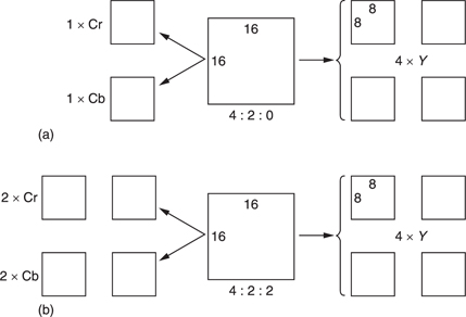
Figure 9.13 The structure of a macroblock. (A macroblock is the screen area steered by one vector.) (a) In 4:2:0, there are two chroma DCT blocks per macroblock whereas in 4:2:2 (b) there are four, 4:2:2 needs 33 per cent more data than 4:2:0.
In the 4:2:2 Profile of MPEG-2, shown in Figure 9.13(b), the chroma is not downsampled vertically, and so there is twice as much chroma data in each macroblock which is otherwise substantially the same.
In MPEG-4 the motion-compensation process is taken further. The macroblock approach of MPEG-2 will always result in prediction errors because object boundaries seldom coincide with macroblock boundaries. MPEG-4 overcomes this limitation because its motion compensation is object based. Essentially in MPEG-4 it is possible to describe an arbitrarily shaped object which can then be steered with vectors.
9.5 I and P coding
Predictive (P) coding cannot be used indefinitely, as it is prone to error propagation. A further problem is that it becomes impossible to decode the transmission if reception begins part-way through. In real video signals, cuts or edits can be present across which there is little redundancy and which make motion estimators throw up their hands.
In the absence of redundancy over a cut, there is nothing to be done but to send the new picture information in absolute form. This is called I coding where I is an abbreviation of intra coding. As I coding needs no previous picture for decoding, then decoding can begin at I coded information.
MPEG is effectively a toolkit and there is no compulsion to use all the tools available. Thus an encoder may choose whether to use I or P coding, either once and for all or dynamically on a macroblock-by-macroblock basis.
For practical reasons, an entire frame may be encoded as I macroblocks periodically. This creates a place where the bitstream might be edited or where decoding could begin.
Figure 9.14 shows a typical application of the Simple Profile of MPEG- 2. Periodically an I picture is created. Between I pictures are P pictures which are based on the picture before. These P pictures predominantly contain macroblocks having vectors and prediction errors. However, it is perfectly legal for P pictures to contain I macroblocks. This might be useful where, for example, a camera pan introduces new material at the edge of the screen which cannot be created from an earlier picture.
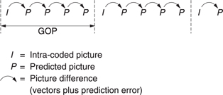
Figure 9.14 A Simple Profile MPEG-2 signal may contain periodic l pictures with a number of P pictures between.
Note that although what is sent is called a P picture, it is not a picture at all. It is a set of instructions to convert the previous picture into the current picture. If the previous picture is lost, decoding is impossible. An I picture together with all of the pictures before the next I picture form a Group of Pictures (GOP).
9.6 Bidirectional coding
Motion-compensated predictive coding is a useful compression technique, but it does have the drawback that it can only take data from a previous picture. Where moving objects reveal a background this is completely unknown in previous pictures and forward prediction fails. However, more of the background is visible in later pictures. Figure 9.15 shows the concept. In the centre of the diagram, a moving object has revealed some background. The previous picture can contribute nothing, whereas the next picture contains all that is required.
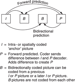
Bidirectional coding is shown inFigure 9.16. A bidirectional or B macroblock can be created using a combination of motion compensation and the addition of a prediction error. This can be done by forward prediction from a previous picture or backward prediction from a subsequent picture. It is also possible to use an average of both forward and backward prediction. On noisy material this may result in some reduction in bit rate. The technique is also a useful way of portraying a dissolve.
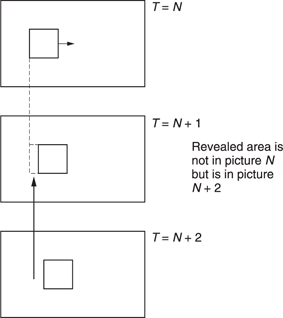
Figure 9.15 In bidirectional coding the revealed background can be efficiently coded by bringing data back from a future picture.
The averaging process in MPEG-2 is a simple linear interpolation which works well when only one B picture exists between the reference pictures before and after. A larger number of B pictures would require weighted interpolation but MPEG-2 does not support this.
Typically two B pictures are inserted between P pictures or between I and P pictures. As can be seen, B pictures are never predicted from one another, only from I or P pictures. A typical GOP for broadcasting purposes might have the structure IBBPBBPBBPBB. Note that the last B pictures in the GOP require the I picture in the next GOP for decoding and so the GOPs are not truly independent. Independence can be obtained by creating a closed GOP which may contain B pictures but which ends with a P picture. It is also legal to have a B picture in which every macroblock is forward predicted, needing no future picture for decoding.
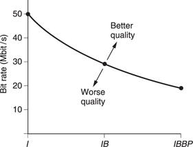
Bidirectional coding is very powerful. Figure 9.17 is a constant quality curve showing how the bit rate changes with the type of coding. On the left, only I or spatial coding is used, whereas on the right an IBBP structure is used. This means that there are two bidirectionally coded pictures in between a spatially coded picture (I) and a forward predicted picture (P). Note how for the same quality the system which only uses spatial coding needs two and a half times the bit rate that the bidirectionally coded system needs.
Clearly information in the future has yet to be transmitted and so is not normally available to the decoder. MPEG-2 gets around the problem by sending pictures in the wrong order. Picture reordering requires delay in the encoder and a delay in the decoder to put the order right again. Thus the overall codec delay must rise when bidirectional coding is used. This is quite consistent with Figure 9.3 which showed that as the compression factor rises the latency must also rise.
Figure 9.18 shows that although the original picture sequence is IBBPBBPBBIBB . . ., this is transmitted as IPBBPBBIBB . . . so that the future picture is already in the decoder before bidirectional decoding begins. Note that the I picture of the next GOP is actually sent before the last B pictures of the current GOP.
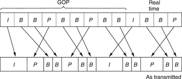
Figure 9.18 Comparison of pictures before and after compression showing sequence change and varying amount of data needed by each picture type. I, P, B pictures use unequal amounts of data.
Figure 9.18 also shows that the amount of data required by each picture is dramatically different. I pictures have only spatial redundancy and so need a lot of data to describe them. P pictures need fewer data because they are created by shifting the I picture with vectors and then adding a prediction error picture. B pictures need the least data of all because they can be created from I or P.
With pictures requiring a variable length of time to transmit, arriving in the wrong order, the decoder needs some help. This takes the form of picture-type flags and time stamps.
9.7 Coding applications
Figure 9.19 shows a variety of GOP structures. The simplest is the III .. sequence in which every picture is intra-coded. Pictures can be fully decoded without reference to any other pictures and so editing is straightforward. However, this approach requires about two and one half times the bit rate of a full bidirectional system. Bidirectional coding is most useful for final delivery of post-produced material either by broadcast or on prerecorded media as there is then no editing requirement. As a compromise the IBIB .. structure can be used which has some of the bit rate advantage of bidirectional coding but without too much latency. It is possible to edit an IBIB stream by performing some processing. If it is required to remove the video following a B picture, that B picture could not be decoded because it needs I pictures either side of it for bidirectional decoding. The solution is to decode the B picture first, and then re-encode it with forward prediction only from the previous I picture. The subsequent I picture can then be replaced by an edit process. Some quality loss is inevitable in this process but this is acceptable in applications such as ENG and industrial video.
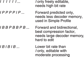
Figure 9.19 Various possible GOP structures used with MPEG. See text for details.
9.8 Spatial compression
Spatial compression in MPEG is used in I pictures on actual picture data and in P and B pictures on prediction error data. MPEG uses the discrete cosine transform described in section 3.7. The DCT works on blocks and in MPEG these are 8 × 8 pixels. Section 5.7 showed how the macroblocks of the motion-compensation structure are designed so they can be broken down into 8 × 8 DCT blocks. In a 4:2:0 macroblock there will be six DCT blocks whereas in a 4:2:2 macroblock there will be eight.
Figure 9.20 shows the table of basis functions or wave table for an 8 × 8 DCT. Adding these two-dimensional waveforms together in different proportions will give any original 8 × 8 pixel block. The coefficients of the DCT simply control the proportion of each wave which is added in the inverse transform. The top-left wave has no modulation at all because it conveys the DC component of the block. This coefficient will be a unipolar (positive only) value in the case of luminance and will typically be the largest value in the block as the spectrum of typical video signals is dominated by the DC component.
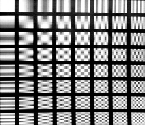
Figure 9.20 The discrete cosine transform breaks up an image area into discrete frequencies in two dimensions. The lowest frequency can be seen here at the top-left corner. Horizontal frequency increases to the right and vertical frequency increases downwards.
Increasing the DC coefficient adds a constant amount to every pixel. Moving to the right the coefficients represent increasing horizontal spatial frequencies and moving downwards the coefficients represent increasing vertical spatial frequencies. The bottom-right coefficient represents the highest diagonal frequencies in the block. All these coefficients are bipolar, where the polarity indicates whether the original spatial waveform at that frequency was inverted.
Figure 9.21 shows a one-dimensional example of an inverse transform. The DC coefficient produces a constant level throughout the pixel block. The remaining waves in the table are AC coefficients. A zero coefficient would result in no modulation, leaving the DC level unchanged. The wave next to the DC component represents the lowest frequency in the transform which is half a cycle per block. A positive coefficient would make the left side of the block brighter and the right side darker whereas a negative coefficient would do the opposite. The magnitude of the coefficient determines the amplitude of the wave which is added. Figure 9.21 also shows that the next wave has a frequency of one cycle per block. i.e. the block is made brighter at both sides and darker in the middle.
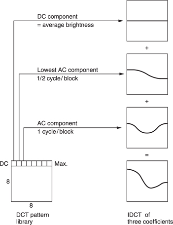
Figure 9.21 A one-dimensional inverse transform. See text for details.
Consequently an inverse DCT is no more than a process of mixing various pixel patterns from the wave table where the relative amplitudes and polarity of these patterns are controlled by the coefficients. The original transform is simply a mechanism which finds the coefficient amplitudes from the original pixel block.
The DCT itself achieves no compression at all. Sixty-four pixels are converted to sixty-four coefficients. However, in typical pictures, not all coefficients will have significant values; there will often be a few dominant coefficients. The coefficients representing the higher twodimensional spatial frequencies will often be zero or of small value in large areas, due to blurring or simply plain undetailed areas before the camera.
Statistically, the further from the top-left corner of the wave table the coefficient is, the smaller will be its magnitude. Coding gain (the technical term for reduction in the number of bits needed) is achieved by transmitting the low-valued coefficients with shorter wordlengths. The zero-valued coefficients need not be transmitted at all. Thus it is not the DCT which compresses the data, it is the subsequent processing. The DCT simply expresses the data in a form which makes the subsequent processing easier.
Higher compression factors require the coefficient wordlength to be further reduced using requantizing. Coefficients are divided by some factor which increases the size of the quantizing step. The smaller number of steps which results permits coding with fewer bits, but of course with an increased quantizing error. The coefficients will be multiplied by a reciprocal factor in the decoder to return to the correct magnitude.
Inverse transforming a requantized coefficient means that the frequency it represents is reproduced in the output with the wrong amplitude. The difference between original and reconstructed amplitude is regarded as a noise added to the wanted data. Figure 9.22 shows that the visibility of such noise is far from uniform. The maximum sensitivity is found at DC and falls thereafter. As a result the top-left coefficient is often treated as a special case and left unchanged. It may warrant more error protection than other coefficients.
MPEG takes advantage of the falling sensitivity to noise. Prior to requantizing, each coefficient is divided by a different weighting constant as a function of its frequency. Figure 9.23 shows a typical weighting process. Naturally the decoder must have a corresponding inverse weighting. This weighting process has the effect of reducing the magnitude of high-frequency coefficients disproportionately. Clearly different weighting will be needed for colour difference data as colour is perceived differently.
P and B pictures are decoded by adding a prediction error image to a reference image. That reference image will contain weighted noise. One purpose of the prediction error is to cancel that noise to prevent tolerance build-up. If the prediction error were also to contain weighted noise this result would not be obtained. Consequently prediction error coefficients are flat weighted.
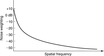
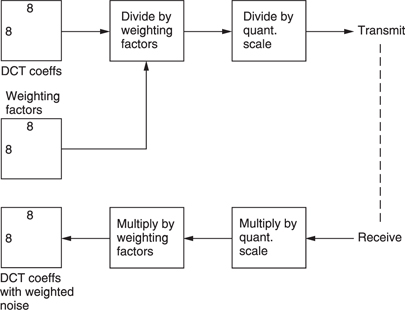
Figure 9.23 Weighting is used to make the noise caused by requantizing different at each frequency.
When forward prediction fails, such as in the case of new material introduced in a P picture by a pan, P coding would set the vectors to zero and encode the new data entirely as an unweighted prediction error. In this case it is better to encode that material as an I macroblock because then weighting can be used and this will require fewer bits.
Requantizing increases the step size of the coefficients, but the inverse weighting in the decoder results in step sizes which increase with frequency. The larger step size increases the quantizing noise at high frequencies where it is less visible. Effectively the noise floor is shaped to match the sensitivity of the eye. The quantizing table in use at the encoder can be transmitted to the decoder periodically in the bitstream.
9.9 Scanning and run-length/variable-length coding
Study of the signal statistics gained from extensive analysis of real material is used to measure the probability of a given coefficient having a given value. This probability turns out to be highly non-uniform, suggesting the possibility of a variable-length encoding for the coefficient values. On average, the higher the spatial frequency, the lower the value of a coefficient will be. This means that the value of a coefficient falls as a function of its radius from the DC coefficient.
Typical material often has many coefficients which are zero valued, especially after requantizing. The distribution of these also follows a pattern. The non-zero values tend to be found in the top-left corner of the DCT block, but as the radius increases, not only do the coefficient values fall, but it becomes increasingly likely that these small coefficients will be interspersed with zero-valued coefficients. As the radius increases further it is probable that a region where all coefficients are zero will be entered.
MPEG uses all these attributes of DCT coefficients when encoding a coefficient block. By sending the coefficients in an optimum order, by describing their values with Huffman coding and by using run-length encoding for the zero-valued coefficients it is possible to achieve a significant reduction in coefficient data which remains entirely lossless. Despite the complexity of this process, it does contibute to improved picture quality because for a given bit rate lossless coding of the coefficients must be better than requantizing, which is lossy. Of course, for lower bit rates both will be required.
It is an advantage to scan in a sequence where the largest coefficient values are scanned first. Then the next coefficient is more likely to be zero than the previous one. With progressively scanned material, a regular zigzag scan begins in the top-left corner and ends in the bottom-right corner as shown in Figure 9.24. Zig-zag scanning means that significant values are more likely to be transmitted first, followed by the zero values. Instead of coding these zeros, an unique ‘end of block’ (EOB) symbol is transmitted instead.
As the zig-zag scan approaches the last finite coefficient it is increasingly likely that some zero value coefficients will be scanned.
Instead of transmitting the coefficients as zeros, the zero-run-length, i.e. the number of zero valued coefficients in the scan sequence is encoded into the next non-zero coefficient which is itself variable-length coded. This combination of run-length and variable-length coding is known as RLC/ VLC in MPEG.
The DC coefficient is handled separately because it is differentially coded and this discussion relates to the AC coefficients. Three items need to be handled for each coefficient: the zero-run-length prior to this coefficient, the wordlength and the coefficient value itself. The wordlength needs to be known by the decoder so that it can correctly parse the bitstream. The wordlength of the coefficient is expressed directly as an integer called the size.
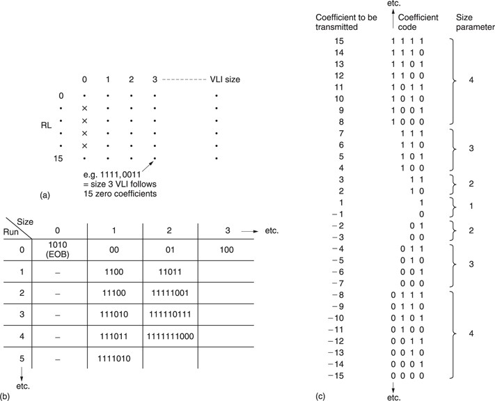
Figure 9.25(a) shows that a two-dimensional run/size table is created. One dimension expresses the zero-run-length; the other the size. A run length of zero is obtained when adjacent coefficients are non-zero, but a code of 0/0 has no meaningful run/size interpretation and so this bit pattern is used for the end-of-block (EOB) symbol.
In the case where the zero-run-length exceeds 14, a code of 15/0 is used signifying that there are fifteen zero-valued coefficients. This is then followed by another run/size parameter whose run-length value is added to the previous fifteen.
The run/size parameters contain redundancy because some combinations are more common than others. Figure 9.25(b) shows that each run/ size value is converted to a variable-length Huffman codeword for transmission. As was shown in section 1.5, the Huffman codes are designed so that short codes are never a prefix of long codes so that the decoder can deduce the parsing by testing an increasing number of bits until a match with the look-up table is found.
Having parsed and decoded the Huffman run/size code, the decoder then knows what the coefficient wordlength will be and can correctly parse that.
The variable-length coefficient code has to describe a bipolar coefficient, i.e one which can be positive or negative. Figure 9.25(c) shows that for a particular size, the coding scale has a certain gap in it. For example, all values from −7 to +7 can be sent by a size 3 code, so a size 4 code only has to send the values of −15 to −8 and +8 to +15. The coefficient code is sent as a pure binary number whose value ranges from all zeros to all ones where the maximum value is a function of the size. The number range is divided into two, the lower half of the codes specifying negative values and the upper half specifying positive.
In the case of positive numbers, the transmitted binary value is the actual coefficient value, whereas in the case of negative numbers a constant must be subtracted which is a function of the size. In the case of a size 4 code, the constant is 1510. Thus a size 4 parameter of 01112 (710) would be interpreted as 7 −15 = −8. A size of 5 has a constant of 31 so a transmitted coded of 010102 (102) would be interpreted as 10 −31 = −21.
This technique saves a bit because, for example, 63 values from −31 to +31 are coded with only five bits having only 32 combinations. This is possible because that extra bit is effectively encoded into the run/size parameter.
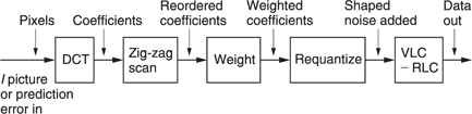
Figure 9.26 A complete spatial coding system which can compress an I picture or the prediction error in P and B pictures. See text for details.
Figure 9.26 shows the whole spatial coding subsystem. Macroblocks are subdivided into DCT blocks and the DCT is calculated. The resulting coefficients are multiplied by the weighting matrix and then requantized. The coefficients are then reordered by the zig-zag scan so that full advantage can be taken of run-length and variable-length coding. The last non-zero coefficient in the scan is followed by the EOB symbol.
In predictive coding, sometimes the motion-compensated prediction is nearly exact and so the prediction error will be almost zero. This can also happen on still parts of the scene. MPEG takes advantage of this by sending a code to tell the decoder there is no prediction error data for the macroblock concerned.
The success of temporal coding depends on the accuracy of the vectors. Trying to reduce the bit rate by reducing the accuracy of the vectors is false economy as this simply increases the prediction error. Consequently for a given GOP structure it is only in the the spatial coding that the overall bit rate is determined. The RLC/VLC coding is lossless and so its contribution to the compression cannot be varied. If the bit rate is too high, the only option is to increase the size of the coefficient-requantizing steps. This has the effect of shortening the wordlength of large coefficients, and rounding small coefficients to zero, so that the bit rate goes down. Clearly if taken too far the picture quality will also suffer because at some point the noise floor will become visible as some form of artifact.
9.10 A bidirectional coder
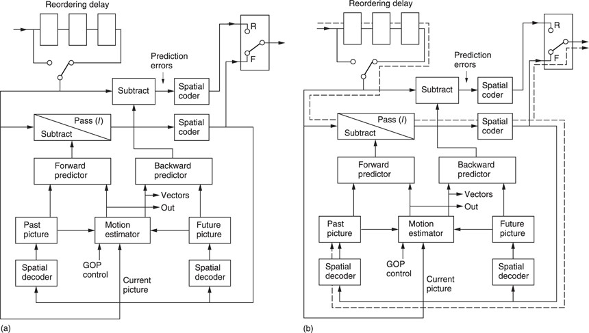
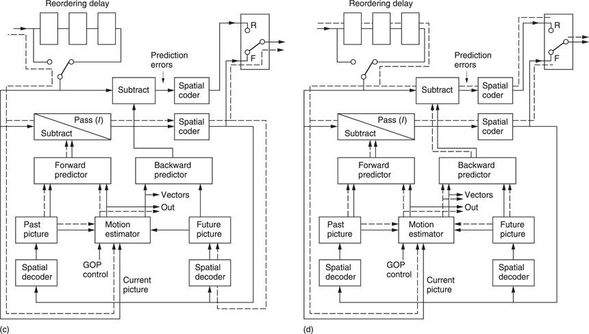
MPEG does not specify how an encoder is to be built or what coding decisions it should make. Instead it specifies the protocol of the bitstream at the output. As a result the MPEG-2 coder shown in Figure 9.27 is only an example.
Figure 9.27(a) shows the component parts of the coder. At the input is a chain of picture stores which can be bypassed for reordering purposes. This allows a picture to be encoded ahead of its normal timing when bidirectional coding is employed.
At the centre is a dual-motion estimator which can simultaneously measure motion between the input picture and earlier picture and a later picture. These reference pictures are held in frame stores. The vectors from the motion estimator are used locally to shift a picture in a frame store to form a predicted picture. This is subtracted from the input picture to produce a prediction error picture which is then spatially coded.
The bidirectional encoding process will now be described. A GOP begins with an I picture which is intra-coded. In Figure 9.27(b) the I picture emerges from the reordering delay. No prediction is possible on an I picture so the motion estimator is inactive. There is no predicted picture and so the prediction error subtractor is set simply to pass the input. The only processing which is active is the forward spatial coder which describes the picture with DCT coefficients. The output of the forward spatial coder is locally decoded and stored in the past picture frame store.
The reason for the spatial encode/decode is that the past picture frame store now contains exactly what the decoder frame store will contain, including the effects of any requantizing errors. When the same picture is used as a reference at both ends of a differential coding system, the errors will cancel out.
Having encoded the I picture, attention turns to the P picture. The input sequence is IBBP, but the transmitted sequence must be IPBB. Figure 9.27(c) shows that the reordering delay is bypassed to select the P picture. This passes to the motion estimator which compares it with the I picture and outputs a vector for each macroblock. The forward predictor uses these vectors to shift the I picture so that it more closely resembles the P picture. The predicted picture is then subtracted from the actual picture to produce a forward prediction error. This is then spatially coded. Thus the P picture is transmitted as a set of vectors and a prediction error image.
The P picture is locally decoded in the right-hand decoder. This takes the forward-predicted picture and adds the decoded prediction error to obtain exactly what the decoder will obtain.
Figure 9.27(d) shows that the encoder now contains an I picture in the left store and a P picture in the right store. The reordering delay is reselected so that the first B picture can be input. This passes to the motion estimator where it is compared with both the I and P pictures to produce forward and backward vectors. The forward vectors go to the forward predictor to make a B prediction from the I picture. The backward vectors go to the backward predictor to make a B prediction from the P picture. These predictions are simultaneously subtracted from the actual B picture to produce a forward prediction error and a backward prediction error. These are then spatially encoded. The encoder can then decide which direction of coding resulted in the best prediction; i.e. the smallest prediction error.
Not shown in the interests of clarity is a third signal path which creates a predicted B picture from the average of forward and backward predictions. This is subtracted from the input picture to produce a third prediction error. In some circumstances this prediction error may use fewer data than either forward or backward prediction alone.
As B pictures are never used to create other pictures, the decoder does not locally decode the B picture. After decoding and displaying the B picture the decoder will discard it. At the encoder the I and P pictures remain in their frame stores and the second B picture is input from the reordering delay.
Following the encoding of the second B picture, the encoder must reorder again to encode the second P picture in the GOP. This will be locally decoded and will replace the I picture in the left store. The stores and predictors switch designation because the left store is now a future P picture and the right store is now a past P picture. B pictures between them are encoded as before.
9.11 Slices
There is still some redundancy in the output of a bidirectional coder and MPEG is remarkably diligent in finding it. In I pictures, the DC coefficient describes the average brightness of an entire DCT block. In real video the DC component of adjacent blocks will be similar much of the time. A saving in bit rate can be obtained by differentially coding the DC coefficient.
In P and B pictures this is not done because these are prediction errors not actual images and the statistics are different. However, P and B pictures send vectors and instead the redundancy in these is explored. In a large moving object, many macroblocks will be moving at the same velocity and their vectors will be the same. Thus differential vector coding will be advantageous.
As has been seen above, differential coding cannot be used indiscriminately as it is prone to error propagation. Periodically absolute DC coefficients and vectors must be sent and the slice is the logical structure which supports this mechanism. In I pictures, the first DC coefficient in a slice is sent in absolute form, whereas the subsequent coefficients are sent differentially. In P or B pictures, the first vector in a slice is sent in absolute form, but the subsequent vectors are differential.
Slices are horizontal picture strips which are one macroblock (16 pixels) high and which proceed from left to right across the screen. The sides of the picture must coincide with the beginning or the end of a slice in MPEG-2, but otherwise the encoder is free to decide how big slices should be and where they begin.
In the case of a central dark building silhouetted against the bright sky, there would be two large changes in the DC coefficients, one at each edge of the building. It may be advantageous to the encoder to break the width of the picture into three slices, one each for the left and right areas of sky and one for the building. In the case of a large moving object, different slices may be used for the object and the background.
Each slice contains its own synchronizing pattern, so following a transmission error, correct decoding can resume at the next slice. Slice size can also be matched to the characteristics of the transmission channel. For example, in an error-free transmission system the use of a large number of slices in a packet simply wastes data capacity on surplus synchronizing patterns. However, in a non-ideal system it might be advantageous to have frequent resynchronizing.
9.12 Handling interlaced pictures
MPEG-1 handles interlaced inputs by discarding alternate fields to produce a non-interlaced signal. In MPEG-2, spatial coding, predictive coding and motion compensation can still be performed using interlaced source material at the cost of considerable complexity. Despite that complexity, coders cannot be expected to perform as well with interlaced material.
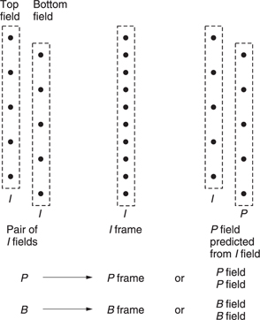
Figure 9.28 shows that in an incoming interlaced frame there are two fields each of which contain half of the lines in the frame. In MPEG-2 these are known as the top field and the bottom field. In video from a camera, these fields represent the state of the image at two different times. Where there is little image motion, this is unimportant and the fields can be combined obtaining more effective compression. However, in the presence of motion the fields become increasingly decorrelated because of the displacement of moving objects from one field to the next.
This characteristic determines that MPEG-2 must be able to handle fields independently or together. This dual approach permeates all aspects of MPEG-2 and affects the definition of pictures, macroblocks, DCT blocks and zig-zag scanning.
Figure 9.28 also shows how MPEG-2 designates interlaced fields. In picture types I, P and B, the two fields can be superimposed to make a frame-picture or the two fields can be coded independently as two field-pictures. As a third possibility, in I pictures only, the bottom field-picture can be predictively coded from the top field-picture to make an IP frame-picture.
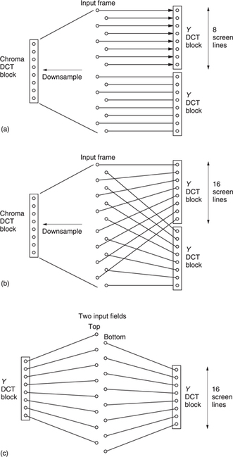
A frame-picture is one in which the macroblocks contain lines from both field types over a picture area 16 scan lines high. Each luminance macroblock contains the usual four DCT blocks but there are two ways in which these can be assembled. Figure 9.29(a) shows how a frame is divided into frame DCT blocks. This is identical to the progressive scan approach in that each DCT block contains eight contiguous picture lines. In 4:2:0, the colour difference signals have been downsampled by a factor of two and shifted as was shown in section 4.18. Figure 9.29(a) also shows how one 4:2:0 DCT block contains the chroma data from 16 lines in two fields.
Even small amounts of motion in any direction can destroy the correlation between odd and even lines and a frame DCT will result in an excessive number of coefficients. Figure 9.29(b) shows that instead the luminance component of a frame can also be divided into field DCT blocks. In this case one DCT block contains odd lines and the other contains even lines. In this mode the chroma still produces one DCT block from both fields as in Figure 9.29(a).
When an input frame is designated as two field-pictures, the macroblocks come from a screen area which is 32 lines high. Figure 9.29(c) shows that the DCT blocks contain the same data as if the input frame had been designated a frame-picture but with field DCT. Consequently it is only frame-pictures which have the option of field or frame DCT. These may be selected by the encoder on a macroblock-by-macroblock basis and, of course, the resultant bitstream must specify what has been done.
In a frame which contains a small moving area, it may be advantageous to encode as a frame-picture with frame DCT except in the moving area where field DCT is used. This approach may result in fewer bits than coding as two field-pictures.
In a field-picture and in a frame-picture using field DCT, a DCT block contains lines from one field type only and this must have come from a screen area sixteen scan lines high, whereas in progressive scan and frame DCT the area is only eight scan lines high. A given vertical spatial frequency in the image is sampled at points twice as far apart which is interpreted by the field DCT as a doubled spatial frequency, whereas there is no change in the horizontal spectrum.
Following the DCT calculation, the coefficient distribution will be different in field-pictures and field DCT frame-pictures. In these cases, the probability of coefficients is not a constant funtion of radius from the DC coefficient as it is in progressive scan, but is elliptical where the ellipse is twice as high as it is wide.
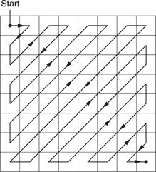
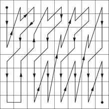
Using the standard 45° zig-zag scan with this different coefficient distribution would not have the required effect of putting all the significant coefficients at the beginning of the scan. To achieve this requires a different zig-zag scan, which is shown in Figure 9.30. This scan, sometimes known as the Yeltsin walk, attempts to match the elliptical probability of interlaced coefficients with a scan slanted at 67.5° to the vertical. This is clearly suboptimal, and is one of the reasons why MPEG-2 does not work so well with interlaced video.
Motion estimation is more difficult in an interlaced system. Vertical detail can result in differences between fields and this reduces the quality of the match. Fields are vertically subsampled without filtering and so contain alias products. This aliasing will mean that the vertical waveform representing a moving object will not be the same in successive pictures and this will also reduce the quality of the match.
Even when the correct vector has been found, the match may be poor so the estimator fails to recognize it. If it is recognized, a poor match means that the quality of the prediction in P and B pictures will be poor and so a large prediction error or residual has to be transmitted. In an attempt to reduce the residual, MPEG-2 allows field-pictures to use motion-compensated prediction from either the adjacent field or from the same field type in another frame. In this case the encoder will use the better match. This technique can also be used in areas of frame-pictures which use field DCT.
The motion compensation of MPEG-2 has half-pixel resolution and this is inherently compatible with an interlace because an interpolator must be present to handle the half-pixel shifts. Figure 9.31(a) shows that in an interlaced system, each field contains half of the frame lines and so interpolating half-way between lines of one field type will actually create values lying on the sampling structure of the other field type. Thus it is equally possible for a predictive system to decode a given field type based on pixel data from the other field type or of the same type.
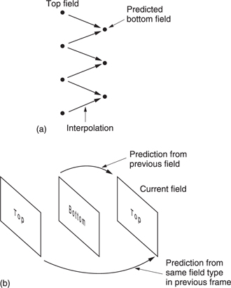
If when using predictive coding from the other field type the vertical motion vector contains a half-pixel component, then no interpolation is needed because the act of transferring pixels from one field to another results in such a shift.
Figure 9.31(b) shows that a macroblock in a given P field-picture can be encoded using a vector which shifts data from the previous field or from the field before that, irrespective of which frames these fields occupy. As noted above, field-picture macroblocks come from an area of screen 32 lines high and this means that the vector density is halved, resulting in larger prediction errors at the boundaries of moving objects.
As an option, field-pictures can restore the vector density by using 16 × 8 motion compensation where separate vectors are used for the top and bottom halves of the macroblock. Frame-pictures can also use 16 × 8 motion compensation in conjunction with field DCT. Whilst the 2 × 2 DCT block luminance structure of a macroblock can easily be divided vertically in two, in 4:2:0 the same screen area is represented by only one chroma macroblock of each component type. As it cannot be divided in half, this chroma is deemed to belong to the luminance DCT blocks of the upper field. In 4:2:2 no such difficulty arises.
MPEG-2 supports interlace simply because interlaced video exists in legacy systems and there is a requirement to compress it. However, where the opportunity arises to define a new system, interlace should be avoided. Legacy interlaced source material should be handled using a motion-compensated de-interlacer prior to compression in the progressive domain.
9.13 An MPEG-2 coder
Figure 9.32 shows a complete MPEG-2 coder. The bidirectional coder outputs coefficients and vectors, and the quantizing table in use. The vectors of P and B pictures and the DC coefficients of I pictures are differentially encoded in slices and the remaining coefficients are RLC/ VLC coded. The multiplexer assembles all these data into a single bitstream called an elementary stream. The output of the encoder is a buffer which absorbs the variations in bit rate between different picture types. The buffer output has a constant bit rate determined by the demand clock. This comes from the transmission channel or storage device. If the bit rate is low, the buffer will tend to fill up, whereas if it is high the buffer will tend to empty. The buffer content is used to control the severity of the requantizing in the spatial coders. The more the buffer fills, the bigger the requantizing steps get.
The buffer in the decoder has a finite capacity and the encoder must model the decoder's buffer occupancy so that it neither overflows nor underflows. An overflow might occur if an I picture is transmitted when the buffer content is already high. The buffer occupancy of the decoder depends somewhat on the memory access strategy of the decoder. Instead of defining a specific buffer size, MPEG-2 defines the size of a particular mathematical model of a hypothetical buffer. The decoder designer can use any strategy which implements the model, and the encoder can use any strategy which doesn't overflow or underflow the model. The elementary stream has a parameter called the video buffer verifier (VBV) which defines the minimum buffering assumptions of the encoder.
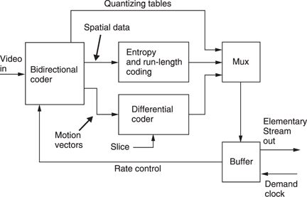
Figure 9.32 An MPEG 2 coder. See text for details.
As was seen above, buffering is one way of ensuring constant quality when picture entropy varies. An intelligent coder may run down the buffer contents in anticipation of a difficult picture sequence so that a large amount of data can be sent.
MPEG does not define what a decoder should do if a buffer underflow or overflow occurs, but since both irrecoverably lose data it is obvious that there will be more or less of an interruption to the decoding. Even a small loss of data may cause loss of synchronization and in the case of long GOP the lost data may make the rest of the GOP undecodable. A decoder may chose to repeat the last properly decoded picture until it can begin to operate correctly again.
Buffer problems occur if the VBV model is violated. If this happens then more than one underflow or overflow can result from a single violation. Switching an MPEG bitstream can cause a violation because the two encoders concerned may have radically different buffer occupancy at the switch.
9.14 The elementary stream
Figure 9.33 shows the structure of the elementary stream from an MPEG- 2 encoder. The structure begins with a set of coefficients representing a DCT block. Six or eight DCT blocks form the luminance and chroma content of one macroblock. In P and B pictures a macroblock will be associated with a vector for motion compensation. Macroblocks are associated into slices in which DC coefficients of I pictures and vectors in P and B pictures are differentially coded. An arbitrary number of slices forms a picture and this needs I/P/B flags describing the type of picture it is. The picture may also have a global vector which efficiently deals with pans.
Several pictures form a Group of Pictures (GOP) and the GOP begins with an I picture and may or may not include P and B pictures in a structure which may vary dynamically.
Several GOPs form a sequence which begins with a sequence header containing important data to help the decoder. It is possible to repeat the header within a sequence, and this helps lock-up in random access applications. The sequence header describes the MPEG-2 profile and level, whether the video is progressive or interlaced, whether the chroma is 4:2:0 or 4:2:2, the size of the picture and the aspect ratio of the pixels. The quantizing matrix used in the spatial coder can also be sent. The sequence begins with a standardized bit pattern which is detected by a decoder to synchronize the deserialization.
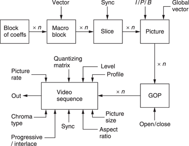
9.15 An MPEG-2 decoder
The decoder is only defined by implication from the definitions of syntax and any decoder which can correctly interpret all combinations of syntax at a particular profile will be deemed compliant however it works.
The first problem a decoder has is that the input is an endless bitstream which contains a huge range of parameters many of which have variable length. Unique synchronizing patterns must be placed periodically throughout the bitstream so that the decoder can identify a known starting point. The pictures which can be sent under MPEG-2 are so flexible that the decoder must first find a sequence header so that it can establish the size of the picture, the frame rate, the colour coding used, etc.
The decoder must also be supplied with a 27 MHz system clock. In a DVD player, this would come from a crystal, but in a transmission system this would be provided by a numerically locked loop running from clock reference parameter in the bitstream (see Chapter 6). Until this loop has achieved lock the decoder cannot function properly.
Figure 9.34 shows a bidirectional decoder. The decoder can only begin decoding with an I picture and as this only uses intra-coding there will be no vectors. An I picture is transmitted as a series of slices. These slices begin with subsidiary synchronizing patterns. The first macroblock in the slice contains an absolute DC coefficient, but the remaining macroblocks code the DC coefficient differentially so the decoder must subtract the differential values from the previous value to obtain the absolute value.
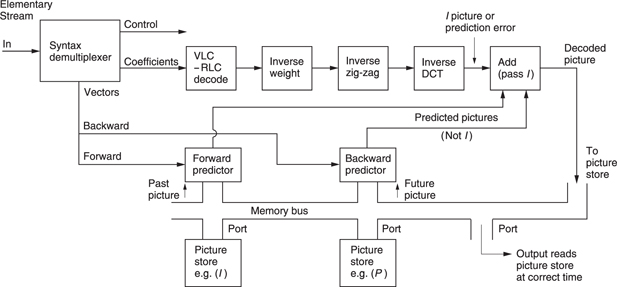
The AC coefficients are sent as Huffman coded run/size parameters followed by coefficient value codes. The variable-length Huffman codes are decoded by using a look-up table and extending the number of bits considered until a match is obtained. This allows the zero-run-length and the coefficient size to be established. The right number of bits is taken from the bitstream corresponding to the coefficient code and this is decoded to the actual coefficient using the size parameter.
If the correct number of bits has been taken from the stream, the next bit must be the beginning of the next run/size code and so on until the EOB symbol is reached. The decoder uses the coefficient values and the zero-run-lengths to populate a DCT coefficient block following the appropriate zig-zag scanning sequence. Following EOB, the bitstream then continues with the next DCT block. Clearly this Huffman decoding will work perfectly or not at all. A single bit slippage in synchronism or a single corrupted data bit can cause a spectacular failure.
Once a complete DCT coefficient block has been received, the coefficients need to be inverse quantized and inverse weighted. Then an inverse DCT can be performed and this will result in an 8 × 8 pixel block. A series of DCT blocks will allow the luminance and colour information for an entire macroblock to be decoded and this can be placed in a framestore. Decoding continues in this way until the end of the slice when an absolute DC coefficient will once again be sent. Once all the slices have been decoded, an entire picture will be resident in the framestore.
The amount of data needed to decode the picture is variable and the decoder just keeps going until the last macroblock is found. It will obtain data from the input buffer. In a constant bit rate transmission system, the decoder will remove more data to decode an I picture than has been received in one picture period, leaving the buffer emptier than it began. Subsequent P and B pictures need much fewer data and allow the buffer to fill again.
The picture will be output when the time stamp (see Chapter 6) sent with the picture matches the state of the decoder's time count.
Following the I picture may be another I picture or a P picture. Assuming a P picture, this will be predictively coded from the I picture. The P picture will be divided into slices as before. The first vector in a slice is absolute, but subsequent vectors are sent differentially. However, the DC coefficients are not differential.
Each macroblock may contain a forward vector. The decoder uses this to shift pixels from the I picture into the correct position for the predicted P picture. The vectors have half-pixel resolution and where a half-pixel shift is required, an interpolator will be used.
The DCT data are sent much as for an I picture. They will require inverse quantizing, but not inverse weighting because P and B coefficients are flatweighted. When decoded this represents an error-cancelling picture which is added pixel-by-pixel to the motion-predicted picture. This results in the output picture.
If bidirectional coding is being used, the P picture may be stored until one or more B pictures have been decoded. The B pictures are sent essentially as a P picture might be, except that the vectors can be forward, backward or bidirectional. The decoder must take pixels from the I picture, the P picture, or both, and shift them according to the vectors to make a predicted picture. The DCT data decodes to produce an error-cancelling image as before.
In an interlaced system, the prediction mechanism may alternatively obtain pixel data from the previous field or the field before that. Vectors may relate to macroblocks or to 16 × 8 pixel areas. DCT blocks after decoding may represent frame lines or field lines. This adds up to a lot of different possibilities for a decoder handling an interlaced input.
9.16 Coding artifacts
This section describes the visible results of imperfect coding. Imperfect coding may be where the coding algorithm is suboptimal, where the coder latency is too short or where the compression factor in use is simply too great for the material.
In motion-compensated systems such as MPEG, the use of periodic intra-fields means that the coding noise varies from picture to picture and this may be visible as noise pumping. Noise pumping may also be visible where the amount of motion changes. If a pan is observed, as the pan speed increases the motion vectors may become less accurate and reduce the quality of the prediction processes. The prediction errors will get larger and will have to be more coarsely quantized. Thus the picture becomes noisier as the pan accelerates and the noise reduces as the pan slows down. The same result may be apparent at the edges of a picture during zooming. The problem is worse if the picture contains fine detail. Panning on grass or trees waving in the wind taxes most coders severely. Camera shake from a hand-held camera also increases the motion vector data and results in more noise as does film weave.
Input video noise or film grain degrades inter-coding as there is less redundancy between pictures and the difference data become larger, requiring coarse quantizing and adding to the existing noise.
Where a codec is really fighting the quantizing may become very coarse and as a result the video level at the edge of one DCT block may not match that of its neighbour. As a result the DCT block structure becomes visible as a mosaicing or tiling effect. Coarse quantizing also causes some coefficients to be rounded up and appear larger than they should be. High-frequency coefficients may be eliminated by heavy quantizing and this forces the DCT to act as a steep-cut low-pass filter. This causes fringeing or ringing around sharp edges and extra shadowy edges which were not in the original. This is most noticeable on text.
Excess compression may also result in colour bleed where fringeing has taken place in the chroma or where high-frequency chroma coefficients have been discarded. Graduated colour areas may reveal banding or posterizing as the colour range is restricted by requantizing. These artifacts are almost impossible to measure with conventional test gear.
Neither noise pumping nor blocking are visible on analog video recorders and so it is nonsense to liken the performance of a codec to the quality of a VCR. In fact noise pumping is extremely objectionable because, unlike steady noise, it attracts attention in peripheral vision and may result in viewing fatigue.
In addition to highly detailed pictures with complex motion, certain types of video signal are difficult for MPEG-2 to handle and will usually result in a higher level of artifacts than usual. Noise has already been mentioned as a source of problems. Timebase error from, for example, VCRs is undesirable because this puts succesive lines in different horizontal positions. A straight vertical line becomes jagged and this results in high spatial frequencies in the DCT process. Spurious coefficients are created which need to be coded.
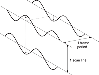
Much archive video is in composite form and MPEG-2 can only handle this after it has been decoded to components. Unfortunately many general-purpose composite decoders have a high level of residual subcarrier in the outputs. This is normally not a problem because the subcarrier is designed to be invisible to the naked eye. Figure 9.35 shows that in PAL and NTSC the subcarrier frequency is selected so that a phase reversal is achieved between successive lines and frames.
Whilst this makes the subcarrier invisible to the eye, it is not invisible to an MPEG decoder. The subcarrier waveform is interpreted as a horizontal frequency, the vertical phase reversals are interpreted as a vertical spatial frequency and the picture-to-picture reversals increase the magnitude of the prediction errors. The subcarrier level may be low but it can be present over the whole screen and require an excess of coefficients to describe it.
Composite video should not in general be used as a source for MPEG-2 encoding, but where this is inevitable the standard of the decoder must be much higher than average, especially in the residual subcarrier specification. Some MPEG preprocessors support high-grade composite decoding options.
Judder from conventional linear standards convertors degrades the performance of MPEG-2. The optic flow axis is corrupted and linear filtering causes multiple images which confuse motion estimators and result in larger prediction errors. If standards conversion is necessary, the MPEG-2 system must be used to encode the signal in its original format and the standards convertor should be installed after the decoder. If a standards convertor has to be used before the encoder, then it must be a type which has effective motion compensation.
Film weave causes movement of one picture with respect to the next and this results in more vector activity and larger prediction errors. Movement of the centre of the film frame along the optical axis causes magnification changes which also result in excess prediction error data. Film grain has the same effect as noise: it is random and so cannot be compressed.
Perhaps because it is relatively uncommon, MPEG-2 cannot handle image rotation well because the motion-compensation system is designed only for translational motion. Where a rotating object is highly detailed, such as in certain fairground rides, the motion-compensation failure requires a significant amount of prediction error data and if a suitable bit rate is not available the level of artifacts will rise.
Flash guns used by still photographers are a serious hazard to MPEG-2 especially when long GOPs are used. At a press conference where a series of flashes may occur, the resultant video contains intermittent white frames which defeat prediction. A huge prediction error is required to turn the previous picture into a white picture, followed by another huge prediction error to return the white frame to the next picture. The output buffer fills and heavy requantizing is employed. After a few flashes the picture has generally gone to tiles.
9.17 Processing MPEG-2 and concatenation
Concatenation loss occurs when the losses introduced by one codec are compounded by a second codec. All practical compressers, MPEG-2 included, are lossy because what comes out of the decoder is not bitidentical to what went into the encoder. The bit differences are controlled so that they have minimum visibility to a human viewer.
MPEG-2 is a toolbox which allows a variety of manipulations to be performed in both the spatial and the temporal domain. There is a limit to the compression which can be used on a single frame, and if higher compression factors are needed, temporal coding will have to be used. The longer the run of pictures considered, the lower the bit rate needed, but the harder it becomes to edit.
The most editable form of MPEG-2 is to use I pictures only. As there is no temporal coding, pure cut edits can be made between pictures. The next best thing is to use a repeating IB structure which is locked to the odd/even field structure. Cut edits cannot be made as the B pictures are bidirectionally coded and need data from both adjacent I pictures for decoding. The B picture has to be decoded prior to the edit and reencoded after the edit. This will cause a small concatenation loss.
Beyond the IB structure processing gets harder. If a long GOP is used for the best compression factor, an IBBPBBP . . . structure results. Editing this is very difficult because the pictures are sent out of order so that bidirectional decoding can be used. MPEG allows closed GOPs where the last B picture is coded wholly from the previous pictures and does not need the I picture in the next GOP. The bitstream can be switched at this point but only if the GOP structures in the two source video signals are synchronized (makes colour framing seem easy). Consequently in practice a long GOP bitstream will need to be decoded prior to any production step. Afterwards it will need to be re-encoded.
This is known as naive concatenation and an enormous pitfall awaits. Unless the GOP structure of the output is identical to and synchronized with the input the results will be disappointing. The worst case is where an I picture is encoded from a picture which was formerly a B picture. It is easy enough to lock the GOP structure of a coder to a single input, but if an edit is made between two inputs, the GOP timings could well be different.
As there are so many structures allowed in MPEG, there will be a need to convert between them. If this has to be done, it should only be in the direction which increases the GOP length and reduces the bit rate. Going the other way is inadvisable. The ideal way of converting from, say, the IB structure of a news system to the IBBP structure of an emission system is to use a recompressor. This is a kind of standards convertor which will give better results than a decode followed by an encode.
The DCT part of MPEG-2 itself is lossless. If all the coefficients are preserved intact an inverse transform yields the same pixel data. Unfortunately this does not yield enough compression for many applications. In practice the coefficients are made less accurate by removing bits, starting at the least significant end and working upwards. This process is weighted, or made progressively more aggressive as spatial frequency increases.
Small-value coefficients may be truncated to zero and large-value coefficients are most coarsely truncated at high spatial frequencies where the effect is least visible.
Figure 9.36(a) shows what happens in the ideal case where two identical coders are put in tandem and synchronized. The first coder quantizes the coefficients to finite accuracy and causes a loss on decoding. However, when the second coder performs the DCT calculation, the coefficients obtained will be identical to the quantized coefficients in the first coder and so if the second weighting and requantizing step is identical the same truncated coefficient data will result and there will be no further loss of quality.7
In practice this ideal situation is elusive. If the two DCTs become nonidentical for any reason, the second requantizing step will introduce further error in the coefficients and the artifact level goes up. Figure 9.36(b) shows that non-identical concatenation can result from a large number of real-world effects.
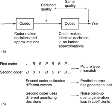
An intermediate processing step such as a fade will change the pixel values and thereby the coefficients. A DVE resize or shift will move pixels from one DCT block to another. Even if there is no processing step, this effect will also occur if the two codecs disagree on where the MPEG picture boundaries are within the picture. If the boundaries are correct there will still be concatenation loss if the two codecs use different weightings.
One problem with MPEG is that the compressor design is unspecified. Whilst this has advantages, it does mean that the chances of finding identical coders is minute because each manufacturer will have his own views on the best compression algorithm. In a large system it may be worth obtaining the coders from a single supplier.
It is now increasingly accepted that concatenation of compression techniques is potentially damaging, and results are worse if the codecs are different. Clearly feeding a digital coder such as MPEG-2 with a signal which has been subject to analog compression comes into the category of worse. Using interlaced video as a source for MPEG coding is suboptimal and using decoded composite video is even worse.
One way of avoiding concatenation is to stay in the compressed data domain. If the goal is just to move pictures from one place to another, decoding to traditional video so an existing router can be used is not ideal, although substantially better than going through the analog domain.
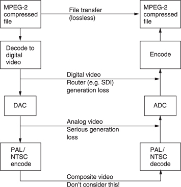
Figure 9.37 shows some possibilities for picture transport. Clearly if the pictures exist as a compressed file on a server, a file transfer is the right way to do it as there is no possibility of loss because there has been no concatenation. File transfer is also quite indifferent to the picture format. It doesn't care whether the pictures are interlaced or not, whether the colour is 4:2:0 or 4:2:2.
Decoding to SDI (serial digital interface) standard is sometimes done so that existing serial digital routing can be used. This is concatenation and has to be done carefully. The compressed video can only use interlace with non-square pixels and the colour coding has to be 4:2:2 because SDI only allows that. If a compressed file has 4:2:0 the chroma has to be interpolated up to 4:2:2 for SDI transfer and then subsampled back to 4:2:0 at the second coder and this will cause generation loss. An SDI transfer also can only be performed in real time, thus negating one of the advantages of compression. In short, traditional SDI is not really at home with compression.
As 4:2:0 progressive scan gains popularity and video production moves steadily towards non-format-specific hardware using computers and data networks, use of the serial digital interface will eventually decline. In the short term, if an existing SDI router has to be used, one solution is to produce a bitstream which is sufficiently similar to SDI that a router will pass it. Systems such as SDDI and ASI (see Chapter 12) work in this way. In short, the signal level, frequency and impedance is pure SDI, but the data protocol is different so that a bit-accurate file transfer can be performed. This has two advantages. First, the compressed data format can be anything appropriate and non-interlaced and/or 4:2:0 can be handled in any picture size, aspect ratio or frame rate. Second, a faster than real-time transfer can be used depending on the compression factor of the file.
An improved way of reducing concatenation loss has emerged from the ATLANTIC research project.8 Figure 9.38 shows that the second encoder in a concatenated scheme does not make its own decisions from the incoming video, but is instead steered by information from the first bitstream. As the second encoder has less intelligence, it is known as a dim encoder.
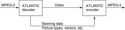
Figure 9.38 In an ATLANTIC system, the second encoder is steered by information from the decoder.
The information bus carries all the structure of the original MPEG-2 bitstream which would be lost in a conventional decoder. The ATLANTIC decoder does more than decode the pictures. It also places on the information bus all parameters needed to make the dim encoder re-enact what the initial MPEG-2 encode did as closely as possible.
The GOP structure is passed on so that pictures are re-encoded as the same type. Positions of macroblock boundaries become identical so that DCT blocks contain the same pixels and motion vectors relate to the same screen data. The weighting and quantizing tables are passed so that coefficient truncation is identical. Motion vectors from the original bitsream are passed on so that the dim encoder does not need to perform motion estimation. In this way predicted pictures will be identical to the original prediction and the prediction error data will be the same.
One application of this approach is in recompression, where an MPEG- 2 bitstream has to have its bit rate reduced. This has to be done by heavier requantizing of coefficients, but if as many other parameters as possible can be kept the same, such as motion vectors, the degradation will be minimized. In a simple recompressor just requantizing the coefficients means that the predictive coding will be impaired. In a proper encode, the quantizing error due to coding, say, an I picture is removed from the P picture by the prediction process. The prediction error of P is obtained by subtracting the decoded I picture rather than the original I picture.
In simple recompression this does not happen and there may be a tolerance build-up known as drift.9 A more sophisticated recompressor will need to repeat the prediction process using the decoded output pictures as the prediction reference.
MPEG-2 bitstreams will often be decoded for the purpose of switching. Local insertion of commercial breaks into a centrally originated bitstream is one obvious requirement. If the decoded video signal is switched, the information bus must also be switched. At the switch point identical reencoding becomes impossible because prior pictures required for predictive coding will have disappeared. At this point the dim encoder has to become bright again because it has to create an MPEG-2 bitstream without assistance.
It is possible to encode the information bus into a form which allows it to be invisibly carried in the serial digital interface. Where a production process such as a vision mixer or DVE performs no manipulation, i.e. becomes bit transparent, the subsequent encoder can extract the information bus and operate in ‘dim’ mode. Where a manipulation is performed, the information bus signal will be corrupted and the encoder has to work in ‘bright’ mode. The encoded information signal is known as a ‘mole’10 because it burrows through the processing equipment!
There will be a generation loss at the switch point because the reencode will be making different decisions in bright mode. This may be difficult to detect because the human visual system is slow to react to a vision cut and defects in the first few pictures after a cut are masked.
In addition to the video computation required to perform a cut, the process has to consider the buffer occupancy of the decoder. A downstream decoder has finite buffer memory, and individual encoders model the decoder buffer occupancy to ensure that it neither overflows nor underflows. At any instant the decoder buffer can be nearly full or nearly empty without a problem provided there is a subsequent correction. An encoder which is approaching a complex I picture may run down the buffer so it can send a lot of data to describe that picture. Figure 9.39(a) shows that if a decoder with a nearly full buffer is suddenly switched to an encoder which has been running down its buffer occupancy, the decoder buffer will overflow when the second encoder sends a lot of data.
An MPEG-2 switcher will need to monitor the buffer occupancy of its own output to avoid overflow of downstream decoders. Where this is a possibility the second encoder will have to recompress to reduce the output bit rate temporarily. In practice there will be a recovery period where the buffer occupancy of the newly selected signal is matched to that of the previous signal. This is shown in Figure 9.39(b).
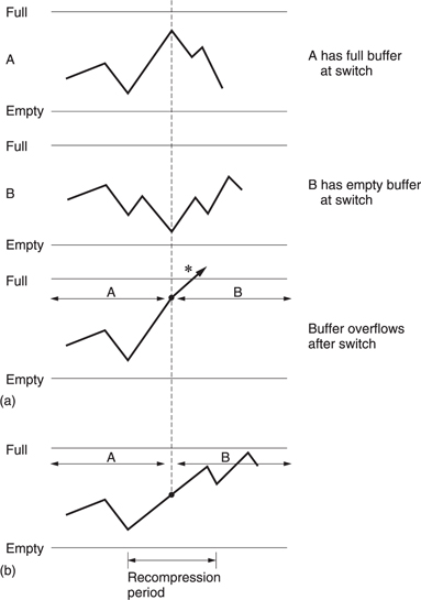
9.18 Audio compression
Perceptive coding relies on the principle of auditory masking, which was considered in Chapter 5. Masking causes the ear/brain combination to be less sensitive to sound at one frequency in the presence of another at a nearby frequency. If a first tone is present in the input, then it will mask signals of lower level at nearby frequencies. The quantizing of the first tone and of further tones at those frequencies can be made coarser. Fewer bits are needed and a coding gain results. The increased quantizing distortion is allowable if it is masked by the presence of the first tone.
The functioning of the ear is noticeably level dependent and perceptive coders take this into account.
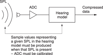
However, all signal processing takes place in the electrical or digital domain with respect to electrical or numerical levels whereas the hearing mechanism operates with respect to true sound pressure level. Figure 9.40 shows that in an ideal system the overall gain of the microphones and ADCs is such that the PCM codes have a relationship with sound pressure which is the same as that assumed by the model in the codec. Equally the overall gain of the DAC and loudspeaker system should be such that the sound pressure levels which the codec assumes are those actually heard. Clearly the gain control of the microphone and the volume control of the reproduction system must be calibrated if the hearing model is to function properly. If, for example, the microphone gain was too low and this was compensated by advancing the loudspeaker gain, the overall gain would be the same but the codec would be fooled into thinking that the sound pressure level was less than it really was and the masking model would not then be appropriate.
The above should come as no surprise as analog audio codecs such as the various Dolby systems have required and implemented line-up procedures and suitable tones. However obvious the need to calibrate coders may be, the degree to which this is recognized in the industry is almost negligible to date and this can only result in suboptimal performance.
9.19 Sound quality measurement
As has been seen, one way in which coding gain is obtained is to requantize sample values to reduce the wordlength. Since the resultant requantizing error is a distortion mechanism it results in energy moving from one frequency to another. The masking model is essential to estimate how audible the effect of this will be. The greater the degree of compression required, the more precise the model must be. If the masking model is inaccurate, then equipment based upon it may produce audible artifacts under some circumstances. Artifacts may also result if the model is not properly implemented. As a result, development of audio compression units requires careful listening tests with a wide range of source material11,12 and precision loudspeakers. The presence of artifacts at a given compression factor indicates only that performance is below expectations; it does not distinguish between the implementation and the model. If the implementation is verified, then a more detailed model must be sought. Naturally comparative listening tests are only valid if all the codecs have been level calibrated and if the loudspeakers cause less loss of information than any of the codecs, a requirement which is frequently overlooked.
Properly conducted listening tests are expensive and time consuming, and alternative methods have been developed which can be used objectively to evaluate the performance of different techniques. The noise to masking ratio (NMR) is one such measurement.13 Figure 9.41 shows how NMR is measured. Input audio signals are fed simultaneously to a data-reduction coder and decoder in tandem and to a compensating delay whose length must be adjusted to match the codec delay. At the output of the delay, the coding error is obtained by subtracting the codec output from the original. The original signal is spectrum-analysed into critical bands in order to derive the masking threshold of the input audio, and this is compared with the critical band spectrum of the error. The NMR in each critical band is the ratio between the masking threshold and the quantizing error due to the codec. An average NMR for all bands can be computed. A positive NMR in any band indicates that artifacts are potentially audible. Plotting the average NMR against time is a powerful technique, as with an ideal codec the NMR should be stable with different types of program material. If this is not the case the codec could perform quite differently as a function of the source material. NMR excursions can be correlated with the waveform of the audio input to analyse how the extra noise was caused and to redesign the codec to eliminate it.
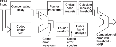
Figure 9.41 The noise-to-masking ratio is derived as shown here.
Practical systems should have a finite NMR in order to give a degree of protection against difficult signals which have not been anticipated and against the use of post-codec equalization or several tandem codecs which could change the masking threshold. There is a strong argument that devices used for audio production should have a greater NMR than consumer or program delivery devices.
9.20 Audio compression tools
There are many different techniques available for audio compression, each having advantages and disadvantages. Real compressors will combine several techniques or tools in various ways to achieve different combinations of cost and complexity. Here it is intended to examine the tools separately before seeing how they are used in actual compression systems.
The simplest coding tool is companding which is a digital parallel of the noise reducers used in analog tape recording. Figure 9.42(a) shows that in companding the input signal level is monitored. Whenever the input level falls below maximum, it is amplified at the coder. The gain which was applied at the coder is added to the data stream so that the decoder can apply an equal attenuation. The advantage of companding is that the signal is kept as far away from the noise floor as possible. In analog noise reduction this is used to maximize the SNR of a tape recorder, whereas in digital compression it is used to keep the signal level as far as possible above the distortion introduced by various coding steps.
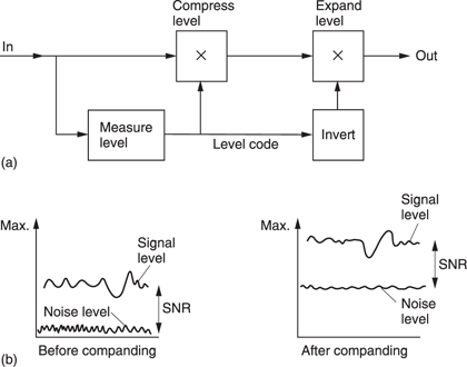
Figure 9.42 Digital companding. In (a) the encoder amplifies the input to maximum level and the decoder attenuates by the same amount. (b) In a companded system, the signal is kept as far as possible above the noise caused by shortening the sample wordlength.
One common way of obtaining coding gain is to shorten the wordlength of samples so that fewer bits need to be transmitted. Figure 9.42(b) shows that when this is done, the distortion will rise by 6 dB for every bit removed. This is because removing a bit halves the number of quantizing intervals which then must be twice as large, doubling the error amplitude.
Clearly if this step follows the compander of (a), the audibility of the distortion will be minimized. As an alternative to shortening the wordlength, the uniform quantized PCM signal can be converted to a non-uniform format. In non-uniform coding, shown at (c), the size of the quantizing step rises with the magnitude of the sample so that the distortion level is greater when higher levels exist.
Companding is a relative of floating-point coding shown in Figure 9.43 where the sample value is expressed as a mantissa and a binary exponent which determines how the mantissa needs to be shifted to have its correct absolute value on a PCM scale. The exponent is the equivalent of the gain setting or scale factor of a compander.
Clearly in floating point the signal-to-noise ratio is defined by the number of bits in the mantissa, and as shown in Figure 9.44, this will vary as a sawtooth function of signal level, as the best value, obtained when the mantissa is near overflow, is replaced by the worst value when the mantissa overflows and the exponent is incremented. Floating-point notation is used within DSP chips as it eases the computational problems involved in handling long wordlengths. For example, when multiplying floating-point numbers, only the mantissae need to be multiplied. The exponents are simply added.
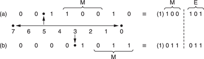
Figure 9.43 In this example of floating-point notation, the radix point can have eight positions determined by the exponent E. The point is placed to the left of the first ‘1’, and the next 4 bits to the right form the mantissa M. As the MSB of the mantissa is always 1, it need not always be stored.
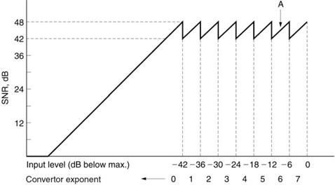
Figure 9.44 In this example of an eight-bit mantissa, three-bit exponent system, the maximum SNR is 6 dB × 8 = 48 dB with maximum input of 0 dB. As input level falls by 6 dB, the convertor noise remains the same, so SNR falls to 42 dB. Further reduction in signal level causes the convertor to shift range (point A in the diagram) by increasing the input analog gain by 6 dB. The SNR is restored, and the exponent changes from 7 to 6 in order to cause the same gain change at the receiver. The noise modulation would be audible in this simple system. A longer mantissa word is needed in practice.
A floating-point system requires one exponent to be carried with each mantissa and this is wasteful because in real audio material the level does not change so rapidly and there is redundancy in the exponents. A better alternative is floating-point block coding, also known as near-instantaneous companding, where the magnitude of the largest sample in a block is used to determine the value of an exponent which is valid for the whole block. Sending one exponent per block requires a lower data rate in than true floating point.14
In block coding the requantizing in the coder raises the quantizing error, but it does so over the entire duration of the block. Figure 9.45 shows that if a transient occurs towards the end of a block, the decoder will reproduce the waveform correctly, but the quantizing noise will start at the beginning of the block and may result in a burst of distortion products (also called pre-noise or pre-echo) which is audible before the transient. Temporal masking may be used to make this inaudible. With a 1 ms block, the artifacts are too brief to be heard.
Another solution is to use a variable time window according to the transient content of the audio waveform. When musical transients occur, short blocks are necessary and the coding gain will be low.15 At other times the blocks become longer allowing a greater coding gain.
Whilst the above systems used alone do allow coding gain, the compression factor has to be limited because little benefit is obtained from masking. This is because the techniques above produce distortion which may be found anywhere over the entire audio band. If the audio input spectrum is narrow, this noise will not be masked.
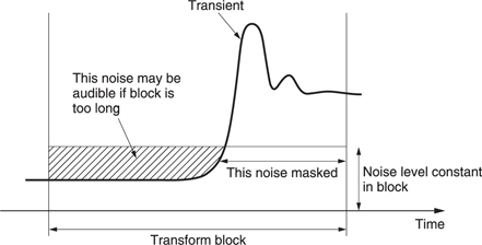
Sub-band coding16 splits the audio spectrum up into many different frequency bands. Once this has been done, each band can be individually processed. In real audio signals many bands will contain lower-level signals than the loudest one. Individual companding of each band will be more effective than broadband companding. Sub-band coding also allows the level of distortion products to be raised selectively so that distortion is only created at frequencies where spectral masking will be effective.
It should be noted that the result of reducing the wordlength of samples in a sub-band coder is often referred to as noise. Strictly, noise is an unwanted signal which is decorrelated from the wanted signal. This is not generally what happens in audio compression. Although the original audio conversion would have been correctly dithered, the linearizing random element in the low-order bits will be some way below the end of the shortened word. If the word is simply rounded to the nearest integer the linearizing effect of the original dither will be lost and the result will be quantizing distortion. As the distortion takes place in a bandlimited system the harmonics generated will alias back within the band. Where the requantizing process takes place in a sub-band, the distortion products will be confined to that sub-band as shown in Figure 9.46. Such distortion is anharmonic.
Following any perceptive coding steps, the resulting data may be further subject to lossless binary compression tools such as prediction, Huffman coding or a combination of both.
Audio is usually considered to be a time-domain waveform as this is what emerges from a microphone. As has been seen in Chapter 3, spectral analysis allows any periodic waveform to be represented by a set of harmonically related components of suitable amplitude and phase. In theory it is perfectly possible to decompose a periodic input waveform into its constituent frequencies and phases, and to record or transmit the transform. The transform can then be inverted and the original waveform will be precisely recreated.
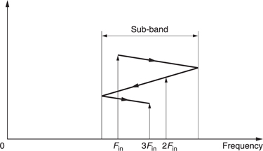
Although one can think of exceptions, the transform of a typical audio waveform changes relatively slowly much of the time. The slow speech of an organ pipe or a violin string, or the slow decay of most musical sounds allow the rate at which the transform is sampled to be reduced, and a coding gain results. At some frequencies the level will be below maximum and a shorter wordlength can be used to describe the coefficient. Further coding gain will be achieved if the coefficients describing frequencies which will experience masking are quantized more coarsely.
In practice there are some difficulties; real sounds are not periodic, but contain transients which transformation cannot accurately locate in time. The solution to this difficulty is to cut the waveform into short segments and then to transform each individually. The delay is reduced, as is the computational task, but there is a possibility of artifacts arising because of the truncation of the waveform into rectangular time windows. A solution is to use window functions, and to overlap the segments as shown in Figure 9.47. Thus every input sample appears in just two transforms, but with variable weighting depending upon its position along the time axis.
Figure 9.47 Transform coding can only be practically performed on short blocks. These are overlapped using window functions in order to handle continuous waveforms.
The DFT (discrete frequency transform) does not produce a continuous spectrum, but instead produces coefficients at discrete frequencies. The frequency resolution (i.e. the number of different frequency coefficients) is equal to the number of samples in the window. If overlapped windows are used, twice as many coefficients are produced as are theoretically necessary. In addition the DFT requires intensive computation, owing to the requirement to use complex arithmetic to render the phase of the components as well as the amplitude. An alternative is to use discrete cosine transforms (DCT) or the modified discrete cosine transform (MDCT) which has the ability to eliminate the overhead of coefficients due to overlapping the windows and return to the critically sampled domain.17 Critical sampling is a term which means that the number of coefficients does not exceed the number which would be obtained with non-overlapping windows.
9.21 Sub-band coding
Sub-band coding takes advantage of the fact that real sounds do not have uniform spectral energy. The wordlength of PCM audio is based on the dynamic range required and this is generally constant with frequency although any pre-emphasis will affect the situation. When a signal with an uneven spectrum is conveyed by PCM, the whole dynamic range is occupied only by the loudest spectral component, and all the other components are coded with excessive headroom. In its simplest form, sub-band coding works by splitting the audio signal into a number of frequency bands and companding each band according to its own level. Bands in which there is little energy result in small amplitudes which can be transmitted with short wordlength. Thus each band results in variablelength samples, but the sum of all the sample wordlengths is less than that of PCM and so a coding gain can be obtained. Sub-band coding is not restricted to the digital domain; the analog Dolby noise-reduction systems use it extensively.
The number of sub-bands to be used depends upon what other compression tools are to be combined with the sub-band coding. If it is intended to optimize compression based on auditory masking, the subbands should preferably be narrower than the critical bands of the ear, and therefore a large number will be required. This requirement is frequently not met: ISO/MPEG Layers I and II use only 32 sub-bands. Figure 9.48 shows the critical condition where the masking tone is at the top edge of the sub-band. It will be seen that the narrower the sub-band, the higher the requantizing ‘noise’ that can be masked. The use of an excessive number of sub-bands will, however, raise complexity and the coding delay, as well as risking pre-ringing on transients which may exceed the temporal masking.
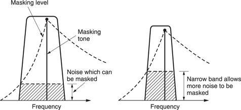
The bandsplitting process is complex and requires a lot of computation. One bandsplitting method which is useful is quadrature mirror filtering. 18 The QMF is is a kind of twin FIR filter which converts a PCM sample stream into two sample streams of half the input sampling rate, so that the output data rate equals the input data rate. The frequencies in the lower half of the audio spectrum are carried in one sample stream, and the frequencies in the upper half of the spectrum are carried in the other. Whilst the lower-frequency output is a PCM band-limited representation of the input waveform, the upper frequency output isn't. A moment's thought will reveal that it could not be so because the sampling rate is not high enough. In fact the upper half of the input spectrum has been heterodyned down to the same frequency band as the lower half by the clever use of aliasing. The waveform is unrecognizable, but when heterodyned back to its correct place in the spectrum in an inverse step, the correct waveform will result once more.
Sampling theory states that the sampling rate needed must be at leasttwice the bandwidth in the signal to be sampled.
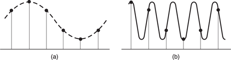
Figure 9.49 The sample stream shown would ordinarily represent the waveform shown in (a), but if it is known that the original signal could exist only between two frequencies then the waveform in (b) must be the correct one. A suitable bandpass reconstruction filter, or synthesis filter, will produce the waveform in (b)..

Figure 9.50 The quadrature mirror filter. At (a) the input spectrum has an audio baseband extending up to half the sampling rate. The input is passed through an FIR low-pass filter which cuts off at one-quarter of the sampling rate to give the spectrum shown at (b). The input also passes in parallel through a second FIR filter whose impulse response has been multiplied by a cosinusoidal waveform in order to amplitude-modulate it. The resultant impulse gives the filter a mirror image frequency response shown at (c). The spectra of both (b) and (c) show that both are oversampled by a factor of two because they are half empty. As a result both can be decimated by a factor of two, resulting at (d) in two identical Nyquist-sampled frequency bands of half the original width.
If the signal is band limited, the sampling rate need only be more than twice the signal bandwidth not the signal frequency. Downsampled signals of this kind can be reconstructed by a reconstruction or synthesis filter having a bandpass response rather than a low-pass response. As only signals within the passband can be output, it is clear from Figure 9.49 that the waveform which will result is the original as the intermediate aliased waveform lies outside the passband.
Figure 9.50 shows the operation of a simple QMF. At (a) the input spectrum of the PCM audio is shown, having an audio baseband extending up to half the sampling rate and the usual lower sideband extending down from there up to the sampling frequency. The input is passed through a FIR low-pass filter which cuts off at one quarter of the sampling rate to give the spectrum shown at (b). The input also passes in parallel through a second FIR filter which is physically identical, but the coefficients are different. The impulse response of the FIR LPF is multiplied by a cosinusoidal waveform which amplitude modulates it. The resultant impulse gives the filter a frequency response shown at (c). This is a mirror image of the LPF response. If certain criteria are met, the overall frequency response of the two filters is flat. The spectra of both (b) and (c) show that both are oversampled by a factor of 2 because they are half-empty. As a result both can be decimated by a factor of two, which is the equivalent of dropping every other sample. In the case of the lower half of the spectrum, nothing remarkable happens. In the case of the upper half of the spectrum, it has been resampled at half the original frequency as shown at (d). The result is that the upper half of the audio spectrum aliases or heterodynes to the lower half.
An inverse QMF will recombine the bands into the original broadband signal. It is a feature of a QMF/inverse QMF pair that any energy near the band edge which appears in both bands due to inadequate selectivity in the filtering reappears at the correct frequency in the inverse filtering process provided that there is uniform quantizing in all the sub-bands. In practical coders, this criterion is not met, but any residual artifacts are sufficiently small to be masked.
The audio band can be split into as many bands as required by cascading QMFs in a tree. However, each stage can only divide the input spectrum in half. In some coders certain sub-bands will have passed through one splitting stage more than others and will be half their bandwidth.19 A delay is required in the wider sub-band data for time alignment.
A simple quadrature mirror is computationally intensive because sample values are calculated which are later decimated or discarded, and an alternative is to use polyphase pseudo-QMF filters20 or wave filters21 in which the filtering and decimation process is combined. Only wanted sample values are computed. A polyphase QMF operates in a manner not unlike the polyphase operation of a FIR filter used for interpolation in sampling rate conversion (see section 3.6). In a polyphase filter a set of samples is shifted into position in the transversal register and then these are multiplied by different sets of coefficients and accumulated in each of several phases to give the value of a number of different samples between input samples. In a polyphase QMF, the same approach is used.
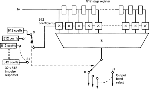
Figure 9.51 shows an example of a 32-band polyphase QMF having a 512-sample window. With 32 sub-bands, each band will be decimated to 1/32 of the input sampling rate. Thus only one sample in 32 will be retained after the combined filter/decimate operation. The polyphase QMF only computes the value of the sample which is to be retained in each subband. The filter works in 32 different phases with the same samples in the transversal register. In the first phase, the coefficients will describe the impulse response of a low-pass filter, the so-called prototype filter, and the result of 512 multiplications will be accumulated to give a single sample in the first band. In the second phase the coefficients will be obtained by multiplying the impulse response of the prototype filter by a cosinusoid at the centre frequency of the second band. Once more 512 multiply accumulates will be required to obtain a single sample in the second band. This is repeated for each of the 32 bands, and in each case a different centre frequency is obtained by multiplying the prototype impulse by a different modulating frequency. Following 32 such computations, 32 output samples, one in each band, will have been computed. The transversal register then shifts 32 samples and the process repeats.
The principle of the polyphase QMF is not so different from the techniques used to compute a frequency transform and effectively blurs the distinction between sub-band coding and transform coding.
The QMF technique is restricted to bands of equal width. It might be thought that this is a drawback because the critical bands of the ear are non-uniform. In fact this is only a problem when very high compression factors are required. In all cases it is the masking model of hearing which must have correct critical bands. This model can then be used to determine how much masking and therefore coding gain is possible within the actual sub-bands used. Uniform width sub-bands will not be able to obtain as much masking as bands which are matched to critical bands, but for many applications the additional coding gain is not worth the added filter complexity.
9.22 Compression formats
There are numerous formats intended for audio compression and these can be divided into international standards and proprietary designs.
The ISO (International Standards Organization) and the IEC (International Electrotechnical Commission) recognized that compression would have an important part to play and in 1988 established the ISO/ IEC/MPEG (Moving Picture Experts Group) to compare and assess various coding schemes in order to arrive at an international standard for compressing video. The terms of reference were extended the same year to include audio and the MPEG/Audio group was formed.
MPEG audio coding is used for DAB (digital audio broadcasting) and for the audio content of digital television broadcasts to the DVB standard.
In the USA, it has been decided to use an alternative compression technique for the audio content of ATSC (Advanced Television Systems Committee) digital television broadcasts. This is the AC-322 system developed by Dolby Laboratories. The MPEG transport stream structure has also been standardized to allow it to carry AC-3 coded audio. The digital video disk can also carry AC-3 or MPEG audio coding.
Other popular proprietary codes include apt-X which is a mild compression factor/short delay codec and ATRAC which is the codec used in MiniDisc.
9.23 MPEG Audio compression
The subject of audio compression was well advanced when the MPEG/ Audio group was formed. As a result it was not necessary for the group to produce ab initio codecs because existing work was considered suitable. As part of the Eureka 147 project, a system known as MUSICAM23 (Masking pattern adapted Universal Sub-band Integrated Coding And Multiplexing) was developed jointly by CCETT in France, IRT in Germany and Philips in the Netherlands. MUSICAM was designed to be suitable for DAB (digital audio broadcasting).
As a parallel development, the ASPEC24 (Adaptive Spectral Perceptual Entropy Coding) system was developed from a number of earlier systems as a joint proposal by AT&T Bell Labs, Thomson, the Fraunhofer Society and CNET. ASPEC was designed for use at high compression factors to allow audio transmission on ISDN.
These two systems were both fully implemented by July 1990 when comprehensive subjective testing took place at the Swedish Broadcasting Corporation.11,25,26As a result of these tests, the MPEG/Audio group combined the attributes of both ASPEC and MUSICAM into a standard27,28 having three levels of complexity and performance.
These three different levels, which are known as layers, are needed because of the number of possible applications. Audio coders can be operated at various compression factors with different quality expectations. Stereophonic classical music requires different quality criteria from monophonic speech. The complexity of the coder will be reduced with a smaller compression factor. For moderate compression, a simple codec will be more cost effective. On the other hand, as the compression factor is increased, it will be necessary to employ a more complex coder to maintain quality.
MPEG Layer I is a simplified version of MUSICAM which is appropriate for the mild compression applications at low cost. Layer II is identical to MUSICAM and is used for DAB and for the audio content of DVB digital television broadcasts. Layer III is a combination of the best features of ASPEC and MUSICAM and is mainly applicable to telecommunications where high compression factors are required.
At each layer, MPEG Audio coding allows input sampling rates of 32, 44.1 and 48 kHz and supports output bit rates of 32, 48, 56, 64, 96, 112, 128, 192, 256 and 384 kbits/s. The transmission can be mono, dual channel (e.g. bilingual), or stereo. Another possibility is the use of joint stereo mode in which the audio becomes mono above a certain frequency. This allows a lower bit rate with the obvious penalty of reduced stereo fidelity.
The layers of MPEG Audio coding (I, II and III ) should not be confused with the MPEG-1 and MPEG-2 television coding standards. MPEG-1 and MPEG-2 flexibly define a range of systems for video and audio coding, whereas the layers define types of audio coding.
The earlier MPEG-1 standard compresses audio and video into about 1.5 Mbits/s.
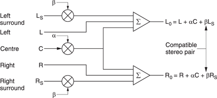
The audio coding of MPEG-1 may be used on its own to encode one or two channels at bit rates up to 448 kbits/s. MPEG-2 allows the number of channels to increase to five: Left, Right, Centre, Left surround, Right surround and Subwoofer. In order to retain reverse compatibility with MPEG-1, the MPEG-2 coding converts the fivechannel input to a compatible two-channel signal, L0, R0, by matrixing29 as shown in Figure 9.52. The data from these two channels are encoded in a standard MPEG-1 audio frame, and this is followed in MPEG-2 by an ancillary data frame which an MPEG-1 decoder will ignore. The ancillary frame contains data for another three audio channels. Figure 9.53 shows that there are eight modes in which these three channels can be obtained. The encoder will select the mode which gives the least data rate for the prevailing distribution of energy in the input channels. An MPEG-2 decoder will extract those three channels in addition to the MPEG-1 frame and then recover all five original channels by an inverse matrix which is steered by mode select bits in the bitstream.
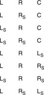
Figure 9.53 In addition to sending the stereo compatible pair, one of the above combinations of signals can be sent. In all cases a suitable inverse matrix can recover the original five channels.
The requirement for MPEG-2 Audio to be backward compatible with MPEG-1 audio coding was essential for some markets, but did compromise the performance because certain useful coding tools could not be used. Consequently the MPEG Audio group evolved a multi-channel standard which was not backward compatible because it incorporated additional coding tools in order to achieve higher performance. This came to be known as MPEG-2 AAC (advanced audio coding).
9.24 MPEG Layer I
Figure 9.54 shows a block diagram of a Layer I coder which is a simplified version of that used in the MUSICAM system. A polyphase filter divides the audio spectrum into 32 equal sub-bands. The output of the filter bank is critically sampled. In other words the output data rate is no higher than the input rate because each band has been heterodyned to a frequency range from zero upwards.

Figure 9.54 A simple sub-band coder. The bit allocation may come from analysis of the sub-band energy, or, for greater reduction, from a spectral analysis in a side chain.
Sub-band compression takes advantage of the fact that real sounds do not have uniform spectral energy. The wordlength of PCM audio is based on the dynamic range required and this is generally constant with frequency although any pre-emphasis will affect the situation. When a signal with an uneven spectrum is conveyed by PCM, the whole dynamic range is occupied only by the loudest spectral component, and all the other components are coded with excessive headroom. In its simplest form, sub-band coding works by splitting the audio signal into a number of frequency bands and companding each band according to its own level. Bands in which there is little energy result in small amplitudes which can be transmitted with short wordlength. Thus each band results in variable-length samples, but the sum of all the sample wordlengths is less than that of the PCM input and so a degree of coding gain can be obtained.
A Layer I compliant encoder, i.e. one whose output can be understood by a standard decoder, can be made which does no more than this. Provided the syntax of the bitstream is correct, the decoder is not concerned with how the coding decisions were made. However, higher compression factors require the distortion level to be increased and this should only be done if it is known that the distortion products will be masked. Ideally the sub-bands should be narrower than the critical bands of the ear. Figure 9.48 showed the critical condition where the masking tone is at the top edge of the sub-band. The use of an excessive number of sub-bands will, however, raise complexity and the coding delay. The use of 32 equal sub-bands in MPEG Layers I and II is a compromise. Efficient polyphase bandsplitting filters can only operate with equalwidth sub-bands and the result, in an octave-based hearing model, is that sub-bands are too wide at low frequencies and too narrow at high frequencies.
To offset the lack of accuracy in the sub-band filter a parallel fast Fourier transform is used to drive the masking model. The standard suggests masking models, but compliant bitstreams can result from other models. In Layer I a 512-point FFT is used. The output of the FFT is used to determine the masking threshold which is the sum of all masking sources. Masking sources include at least the threshold of hearing which may locally be raised by the frequency content of the input audio. The degree to which the threshold is raised depends on whether the input audio is sinusoidal or atonal (broadband, or noise-like).
In the case of a sine wave, the magnitude and phase of the FFT at each frequency will be similar from one window to the next, whereas if the sound is atonal the magnitude and phase information will be chaotic. The masking threshold is a effectively a graph of just noticeable noise as a function of frequency. Figure 9.55(a) shows an example. The masking threshold is calculated by convolving the FFT spectrum with the cochlea spreading function (see section 5.6) with corrections for tonality. The level of the masking threshold cannot fall below the absolute masking threshold which is the threshold of hearing.
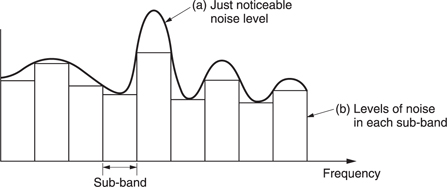
The masking threshold is then superimposed on the actual frequencies of each sub-band so that the allowable level of distortion in each can be established. This is shown in Figure 9.55(b).
Constant size input blocks are used, containing 384 samples. At 48 kHz, 384 samples corresponds to a period of 8 ms. After the sub-band filter each band contains 12 samples per block. The block size is too long to avoid the pre-masking phenomenon of Figure 9.45. Consequently the masking model must ensure that heavy requantizing is not used in a block which contains a large transient following a period of quiet. This can be done by comparing parameters of the current block with those of the previous block as a significant difference will indicate transient activity. The samples in each sub-band block or bin are companded according to the peak value in the bin. A six-bit scale factor is used for each sub-band which applies to all 12 samples. The gain step is 2 dB and so with a six-bit code over 120 dB of dynamic range is available.
A fixed output bit rate is employed, and as there is no buffering the size of the coded output block will be fixed. The wordlengths in each bin will have to be such that the sum of the bits from all the sub-bands equals the size of the coded block. Thus some sub-bands can have long wordlength coding if others have short wordlength coding. The process of determining the requantization step size, and hence the wordlength in each subband, is known as bit allocation. In Layer I all sub-bands are treated in the same way and fourteen different requantization classes are used. Each one has an odd number of quantizing intervals so that all codes are referenced to a precise zero level.
Where masking takes place, the signal is quantized more coarsely until the distortion level is raised to just below the masking level. The coarse quantization requires shorter wordlengths and allows a coding gain. The bit allocation may be iterative as adjustments are made to obtain an equal NMR across all sub-bands. If the allowable data rate is adequate, a positive NMR will result and the decoded quality will be optimal. However, at lower bit rates and in the absence of buffering a temporary increase in bit rate is not possible. The coding distortion cannot be masked and the best the encoder can do is to make the (negative) NMR equal across the spectrum so that artifacts are not emphasized unduly in any one sub-band. It is possible that in some sub-bands there will be no data at all, either because such frequencies were absent in the program material or because the encoder has discarded them to meet a low bit rate.
The samples of differing wordlength in each bin are then assembled into the output coded block. Unlike a PCM block, which contains samples of fixed wordlength, a coded block contains many different wordlengths which may vary from one sub-band to the next. In order to deserialize the block into samples of various wordlength and demultiplex the samples into the appropriate frequency bins, the decoder has to be told what bit allocations were used when it was packed, and some synchronizing means is needed to allow the beginning of the block to be identified.
The compression factor is determined by the bit-allocation system. It is trivial to change the output block size parameter to obtain a different compression factor. If a larger block is specified, the bit allocator simply iterates until the new block size is filled. Similarly the decoder need only deserialize the larger block correctly into coded samples and then the expansion process is identical except for the fact that expanded words contain less noise. Thus codecs with varying degrees of compression are available which can perform different bandwidth/performance tasks with the same hardware.
Figure 9.56(a) shows the format of the Layer I elementary stream. The frame begins with a sync pattern to reset the phase of deserialization, and a header which describes the sampling rate and any use of pre-emphasis. Following this is a block of 32 four-bit allocation codes. These specify the wordlength used in each sub-band and allow the decoder to deserialize the sub-band sample block. This is followed by a block of 32 six-bit scale factor indices, which specify the gain given to each band during companding. The last block contains 32 sets of 12 samples. These samples vary in wordlength from one block to the next, and can be from 0 to fifteen bits long. The deserializer has to use the 32 allocation information codes to work out how to deserialize the sample block into individual samples of variable length.
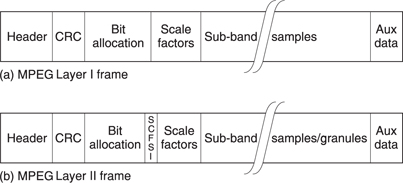
The Layer I MPEG decoder is shown in Figure 9.57. The elementary stream is deserialized using the sync pattern and the variable length samples are assembled using the allocation codes. The variable length samples are returned to fifteen-bit wordlength by adding zeros. The scale factor indices are then used to determine multiplication factors used to return the waveform in each sub-band to its original amplitude. The 32 sub-band signals are then merged into one spectrum by the synthesis filter. This is a set of bandpass filters which heterodynes every sub-band to the correct place in the audio spectrum and then adds them to produce the audio output.
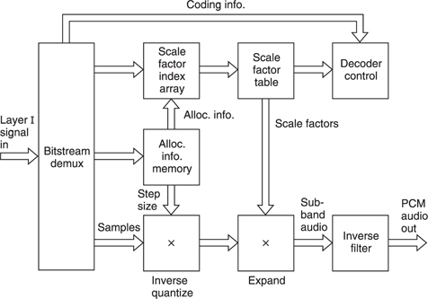
Figure 9.57 The Layer I decoder. See text for details.
9.25 MPEG Layer II
MPEG Layer II audio coding is identical to MUSICAM. The same 32-band filterbank and the same block companding scheme as Layer I is used. In order to give the masking model better spectral resolution, the side chain FFT has 1024 points. The FFT drives the masking model which may be the same as is suggested for Layer I. The block length is increased to 1152 samples. This is three times the block length of Layer I, corresponding to 24 ms at 48 kHz.
Figure 9.56(b) shows the Layer II elementary stream structure. Following the sync pattern the bit-allocation data are sent. The requantizing process of Layer II is more complex than in Layer I. The sub-bands are categorized into three frequency ranges, low, medium and high, and the requantizing in each range is different. Low-frequency samples can be quantized into fifteen different wordlengths, mid-frequencies into seven different wordlengths and high frequencies into only three different wordlengths. Accordingly the bit-allocation data uses words of four, three and two bits depending on the sub-band concerned. This reduces the amount of allocation data to be sent. In each case one extra combination exists in the allocation code. This is used to indicate that no data are being sent for that sub-band.
The 1152 sample block of Layer II is divided into three blocks of 384 samples so that the same companding structure as Layer I can be used. The 2 dB step size in the scale factors is retained. However, not all the scale factors are transmitted, because they contain a degree of redundancy. In real program material, the difference between scale factors in successive blocks in the same band exceeds 2 dB less than 10 per cent of the time. Layer II coders analyse the set of three successive scale factors in each sub-band. On a stationary program, these will be the same and only one scale factor out of three is sent. As the transient content increases in a given sub-band, two or three scale factors will be sent. A two-bit code known as SCFSI (scale factor select information) must be sent to allow the decoder to determine which of the three possible scale factors have been sent for each sub-band. This technique effectively halves the scale factor bit rate.
As for Layer I, the requantizing process always uses an odd number of steps to allow a true centre zero step. In long wordlength codes this is not a problem, but when three, five or nine quantizing intervals are used, binary is inefficient because some combinations are not used. For example, five intervals need a three-bit code having eight combinations leaving three unused.
The solution is that when three, five or nine-level coding is used in a sub-band, sets of three samples are encoded into a granule. Figure 9.58 shows how granules work. Continuing the example of five quantizing intervals, each sample could have five different values, therefore all combinations of three samples could have 125 different values. As 128 values can be sent with a seven-bit code, it will be seen that this is more efficient than coding the samples separately as three five-level codes would need nine bits. The three requantized samples are used to address a look-up table which outputs the granule code. The decoder can establish that granule coding has been used by examining the bitallocation data.
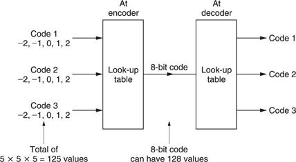
The requantized samples/granules in each sub-band, bit-allocation data, scale factors and scale factor select codes are multiplexed into the output bit stream.
The Layer II decoder is shown in Figure 9.59. This is not much more complex than the Layer I decoder. The demultiplexing will separate the sample data from the side information. The bit-allocation data will specify the wordlength or granule size used so that the sample block can be deserialized and the granules decoded. The scale factor select information will be used to decode the compressed scale factors to produce one scale factor per block of 384 samples. Inverse quantizing and inverse sub-band filtering takes place as for Layer I.
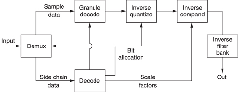
Figure 9.59 A Layer II decoder is slightly more complex than the Layer I decoder because of the need to decode granules and scale factors.
9.26 MPEG Layer III
Layer III is the most complex layer, and is only really necessary when the most severe data rate constraints must be met. It is also known as MP3 in its application of music delivery over the Internet. It is a transform code based on the ASPEC system with certain modifications to give a degree of commonality with Layer II. The original ASPEC coder used a direct MDCT on the input samples. In Layer III this was modified to use a hybrid transform incorporating the existing polyphase 32-band QMF of Layers I and II and retaining the block size of 1152 samples. In Layer 3, the 32 sub-bands from the QMF are further processed by a critically sampled MDCT.
The windows overlap by two to one. Two window sizes are used to reduce pre-echo on transients. The long window works with 36 sub-band samples corresponding to 24 ms, at 48 kHz and resolves eighteen different frequencies, making 576 frequencies altogether. Coding products are spread over this period which is acceptable in stationary material but not in the vicinity of transients. In this case the window length is reduced to 8 ms. Twelve sub-band samples are resolved into six different frequencies making a total of 192 frequencies. This is the Heisenberg inequality: by increasing the time resolution by a factor of three, the frequency resolution has fallen by the same factor.
Figure 9.60 shows the available window types. In addition to the long and short symmetrical windows there is a pair of transition windows, know as start and stop windows which allow a smooth transition between the two window sizes. In order to use critical sampling, MDCTs must resolve into a set of frequencies which is a multiple of four. Switching between 576 and 192 frequencies allows this criterion to be met. Note that an 8 ms window is still too long to eliminate pre-echo. Preecho is eliminated using buffering. The use of a short window minimizes the size of the buffer needed.
Layer III provides a suggested (but not compulsory) pychoacoustic model which is more complex than that suggested for Layers I and II, primarily because of the need for window switching. Pre-echo is associated with the entropy in the audio rising above the average value and this can be used to switch the window size. The perceptive model is used to take advantage of the high-frequency resolution available from the DCT which allows the noise floor to be shaped much more accurately than with the 32 sub-bands of Layers I and II. Although the MDCT has high frequency resolution, it does not carry the phase of the waveform in an identifiable form and so is not useful for discriminating between tonal and atonal inputs. As a result a side FFT which gives conventional amplitude and phase data is still required to drive the masking model.
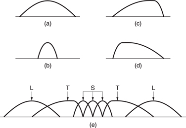
Non-uniform quantizing is used, in which the quantizing step size becomes larger as the magnitude of the coefficient increases. The quantized coefficients are then subject to Huffman coding. This is a technique where the most common code values are allocated the shortest wordlength. Layer III also has a certain amount of buffer memory so that pre-echo can be avoided during entropy peaks despite a constant output bit rate.
Figure 9.61 shows a Layer III encoder. The output from the sub-band filter is 32 continuous band-limited sample streams. These are subject to 32 parallel MDCTs. The window size can be switched individually in each sub-band as required by the characteristics of the input audio. The parallel FFT drives the masking model which decides on window sizes as well as producing the masking threshold for the coefficient quantizer. The distortion control loop iterates until the available output data capacity is reached with the most uniform NMR.
The available output capacity can vary owing to the presence of the buffer. Figure 9.62 shows that the buffer occupancy is fed back to the quantizer. During stationary program material, the buffer contents are deliberately run down by slight coarsening of the quantizing. The buffer empties because the output rate is fixed but the input rate has been reduced. When a transient arrives, the large coefficients which result can be handled by filling the buffer, avoiding raising the output bit rate whilst also avoiding the pre-echo which would result if the coefficients were heavily quantized.
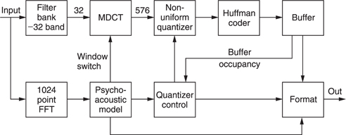
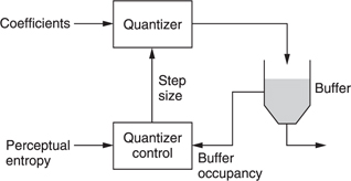
Figure 9.62 The variable rate coding of Layer III. An approaching transient via the perceptual entropy signal causes the coder to quantize more heavily in order to empty the buffer. When the transient arrives, the quantizing can be made more accurate and the increased data can be accepted by the buffer.
In order to maintain synchronism between encoder and decoder in the presence of buffering, headers and side information are sent synchronously at frame rate. However, the position of boundaries between the main data blocks which carry the coefficients can vary with respect to the position of the headers in order to allow a variable frame size. Figure 9.63 shows that the frame begins with an unique sync pattern which is followed by the side information. The side information contains a parameter called main data begin which specifies where the main data for the present frame began in the transmission. This parameter allows the decoder to find the coefficient block in the decoder buffer. As the frame headers are at fixed locations, the main data blocks may be interrupted by the headers.
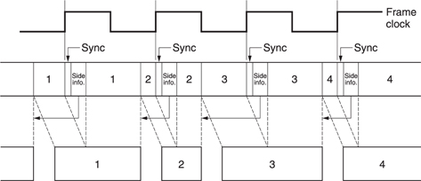
Figure 9.63 In Layer III, the logical frame rate is constant and is transmitted by equally spaced sync patterns. The data blocks do not need to coincide with sync. A pointer after each sync pattern specifies where the data block starts. In this example block 2 is smaller whereas 1 and 3 have enlarged.
9.27 MPEG-2 AAC
The MPEG standards system subsequently developed an enhanced system known as advanced audio coding (AAC).30,31 This was intended to be a standard which delivered the highest possible performance using newly developed tools that could not be used in any standard which was backward compatible. AAC also forms the core of the audio coding of MPEG-4.
AAC supports up to 48 audio channels with default support of monophonic, stereo and 5.1 channel (3/2) audio. The AAC concept is based on a number of coding tools known as modules which can be combined in different ways to produce bitstreams at three different profiles.
The main profile requires the most complex encoder which makes use of all the coding tools. The low-complexity (LC) profile omits certain tools and restricts the power of others to reduce processing and memory requirements. The remaining tools in LC profile coding are identical to those in main profile such that a main profile decoder can decode LC profile bitstreams.
The scaleable sampling rate (SSR) profile splits the input audio into four equal frequency bands each of which results in a self-contained bitstream. A simple decoder can decode only one, two or three of these bitstreams to produce a reduced bandwidth output. Not all the AAC tools are available to SSR profile.
The increased complexity of AAC allows the introduction of lossless coding tools. These allow a lower bit rate for the same or improved quality at a given bit rate where the reliance on lossy coding is reduced. There is greater attention given to the interplay between time-domain and frequency-domain precision in the human hearing system.
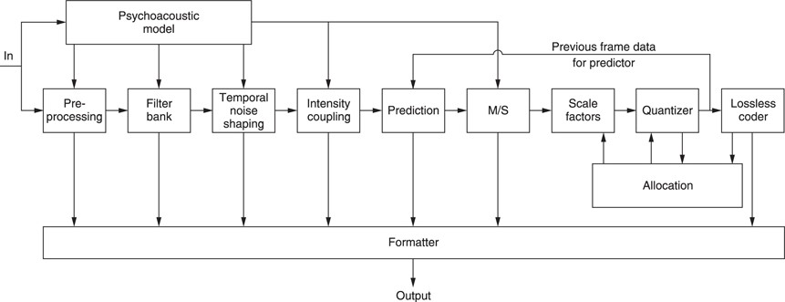
Figure 9.64 shows a block diagram of an AAC main profile encoder. The audio signal path is straight through the centre. The formatter assembles any side-chain data along with the coded audio data to produce a compliant bitstream. The input signal passes to the filter bank and the perceptual model in parallel.
The filter bank consists of a 50 per cent overlapped critically sampled MDCT which can be switched between block lengths of 2048 and 256 samples. At 48 kHz the filter allows resolutions of 23 Hz and 21 ms or 187 Hz and 2.6 ms. As AAC is a multichannel coding system, block length switching cannot be done indiscriminately as this would result in loss of block phase between channels. Consequently if short blocks are selected, the coder will remain in short block mode for integer multiples of eight blocks. This is illustrated in Figure 9.65 which also shows the use of transition windows between the block sizes as was done in Layer III.
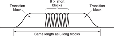
Figure 9.65 In AAC short blocks must be used in multiples of 8 so that the long block phase is undisturbed. This keeps block synchronism in multichannel systems.
The shape of the window function interferes with the frequency selectivity of the MDCT. In AAC it is possible to select either a sine window or a Kaiser-Bessel derived (KBD) window as a function of the input audio spectrum. As was seen in Chapter 3, filter windows allow different compromises between bandwidth and rate of roll-off. The KBD window rolls off later but is steeper and thus gives better rejection of frequencies more than about 200 Hz apart, whereas the sine window rolls off earlier but less steeply and so gives better rejection of frequencies less than 70 Hz.
Following the filter bank is the intra-block predictive coding module. When enabled this module finds redundancy between the coefficients within one transform block. In Chapter 3 the concept of transform duality was introduced, in which a certain characteristic in the frequency domain would be accompanied by a dual characteristic in the time domain and vice versa. Figure 9.66 shows that in the time domain, predictive coding works well on stationary signals but fails on transients. The dual of this characteristic is that in the frequency domain, predictive coding works well on transients but fails on stationary signals.
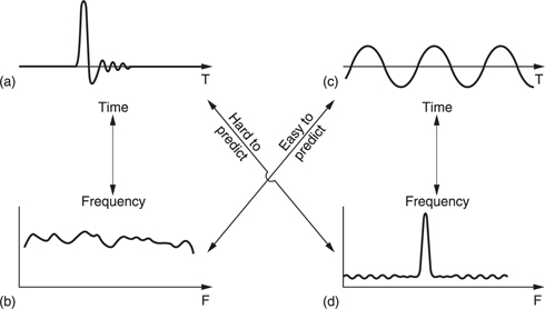
Figure 9.66 Transform duality suggests that predictability will also have a dual characteristic. A time predictor will not anticipate the transient in (a), whereas the broad spectrum of signal (a), shown in (b), will be easy for a predictor advancing down the frequency axis. In contrast, the stationary signal (c) is easy for a time predictor, whereas in the spectrum of (c) shown at (d) the spectral spike will not be predicted.
Equally, a predictive coder working in the time domain produces an error spectrum which is related to the input spectrum. The dual of this characteristic is that a predictive coder working in the frequency domain produces a prediction eror which is related to the input time domain signal.
This explains the use of the term temporal noise shaping (TNS) used in the AAC documents.32 When used during transients, the TNS module produces distortion which is time-aligned with the input such that preecho is avoided. The use of TNS also allows the coder to use longer blocks more of the time. This module is responsible for a significant amount of the increased performance of AAC.
Figure 9.67 shows that the coefficients in the transform block are serialized by a commutator. This can run from the lowest frequency to the highest or in reverse. The prediction method is a conventional forward predictor structure in which the result of filtering a number of earlier coefficients (20 in main profile) is used to predict the current one. The prediction is subtracted from the actual value to produce a prediction error or residual which is transmitted. At the decoder, an identical predictor produces the same prediction from earlier coefficient values and the error in this is cancelled by adding the residual.
Following the intra-block prediction, an optional module known as the intensity/coupling stage is found. This is used for very low bit rates where spatial information in stereo and surround formats is discarded to keep down the level of distortion. Effectively over at least part of the spectrum a mono signal is transmitted along with amplitude codes which allow the signal to be panned in the spatial domain at the decoder.
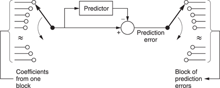
The next stage is the inter-block prediction module. Whereas the intrablock predictor is most useful on transients, the inter-block predictor module explores the redundancy between successive blocks on stationary signals.33 This prediction only operates on coefficients below 16 kHz. For each DCT coefficient in a given block, the predictor uses the quantized coefficients from the same locations in two previous blocks to estimate the present value. As before, the prediction is subtracted to produce a residual which is transmitted. Note that the use of quantized coefficients to drive the predictor is necessary because this is what the decoder will have to do.
The predictor is adaptive and calculates its own coefficients from the signal history. The decoder uses the same algorithm so that the two predictors always track. The predictors run all the time whether prediction is enabled or not in order to keep the prediction coefficients adapted to the signal.
Audio coefficients are associated into sets known as scale factor bands for later companding. Within each scale factor band inter-block prediction can be turned on or off depending on whether a coding gain results.
Protracted use of prediction makes the decoder prone to bit errors and drift and removes decoding entry points from the bitstream. Consequently the prediction process is reset cyclically. The predictors are assembled into groups of 30 and after a certain number of a frames a different group is reset until all have been reset. Predictor reset codes are transmitted in the side data. Reset will also occur if short frames are selected.
In stereo and 3/2 surround formats there is less redundancy because the signals also carry spatial information. The effecting of masking may be up to 20 dB less when distortion products are at a different location in the stereo image from the masking sounds. As a result stereo signals require much higher bit rate than two mono channels, particularly on transient material which is rich in spatial clues.
In some cases a better result can be obtained by converting the signal to a mid-side (M/S) or sum/difference format before quantizing. In surround sound the M/S coding can be applied to the front L/R pair and the rear L/R pair of signals.
In some cases a better result can be obtained by converting the signal to a mid-side (M/S) or sum/difference format before quantizing. In surround sound the M/S coding can be applied to the front L/R pair and the rear L/R pair of signals.
Next comes the lossy stage of the coder where distortion is selectively introduced as a function of frequency as determined by the masking threshold. This is done by a combination of amplification and requantizing. As mentioned, coefficients (or residuals) are grouped into scale factor bands. As Figure 9.68 shows, the number of coefficients varies in order to divide the coefficients into approximate critical bands. Within each scale factor band, all coefficients will be multiplied by the same scale factor prior to requantizing. Coefficients which have been multiplied by a large scale factor will suffer less distortion by the requantizer whereas those which have been multiplied by a small scale factor will have more distortion. Using scale factors, the psychoacoustic model can shape the distortion as a function of frequency so that it remains masked. The scale factors allow gain control in 1.5 dB steps over a dynamic range equivalent to twenty-four-bit PCM and are transmitted as part of the side data so that the decoder can re-create the correct magnitudes.
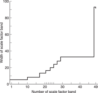
Figure 9.68 In AAC the fine-resolution coefficients are grouped together to form scale factor bands. The size of these varies to loosely mimic the width of critical bands.
The scale factors are differentially coded with respect to the first one in the block and the differences are then Huffman coded.
The requantizer uses non-uniform steps which give better coding gain and has a range of ±8191. The global step size (which applies to all scale factor bands) can be adjusted in 1.5 dB steps. Following requantizing the coefficients are Huffman coded.
There are many ways in which the coder can be controlled and any that results in a compliant bitstream is acceptable although the highest performance may not be reached. The requantizing and scale factor stages will need to be controlled in order to make best use of the available bit rate and the buffering. This is non-trivial because of the use of Huffman coding after the requantizer makes it impossible to predict the exact amount of data which will result from a given step size. This means that the process must iterate.
Whatever bit rate is selected, a good encoder will produce consistent quality by selecting window sizes, intra- or inter-frame prediction and using the buffer to handle entropy peaks. This suggests a connection between buffer occupancy and the control system. The psychoacoustic model will analyse the incoming audio entropy and during periods of average entropy it will empty the buffer by slightly raising the quantizer step size so that the bit rate entering the buffer falls. By running the buffer down, the coder can temporarily support a higher bit rate to handle transients or difficult material.
Simply stated, the scale factor process is controlled so that the distortion spectrum has the same shape as the masking threshold and the quantizing step size is controlled to make the level of the distortion spectrum as low as possible within the allowed bit rate. If the bit rate allowed is high enough, the distortion products will be masked.
9.28 Dolby AC-3
Dolby AC-322 is in fact a family of transform coders based on timedomain aliasing cancellation (TDAC) which allow various compromises between coding delay and bit rate to be used. In the modified discrete cosine transform (MDCT), windows with 50 per cent overlap are used. Thus twice as many coefficients as necessary are produced. These are subsampled by a factor of two to give a critically sampled transform, which results in potential aliasing in the frequency domain. However, by making a slight change to the transform, the alias products in the second half of a given window are equal in size but of opposite polarity to the alias products in the first half of the next window, and so will be cancelled on reconstruction. This is the principle of TDAC.
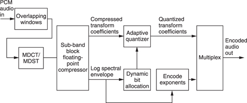
Figure 9.69 shows the generic block diagram of the AC-3 coder. Input audio is divided into 50 per cent overlapped blocks of 512 samples. These are subject to a TDAC transform which uses alternate modified sine and cosine transforms. The transforms produce 512 coefficients per block, but these are redundant and after the redundancy has been removed there are 256 coefficients per block.
The input waveform is constantly analysed for the presence of transients and if these are present the block length will be halved to prevent pre-noise. This halves the frequency resolution but doubles the temporal resolution.
The coefficients have high frequency resolution and are selectively combined in sub-bands which approximate the critical bands. Coefficients in each sub-band are normalized and expressed in floating-point block notation with common exponents. The exponents in fact represent the logarithmic spectral envelope of the signal and can be used to drive the perceptive model which operates the bit allocation. The mantissae of the transform coefficients are then requantized according to the bit allocation.
The output bitstream consists of the requantized coefficients and the log spectral envelope in the shape of the exponents. There is a great deal of redundancy in the exponents. In any block, only the first exponent, corresponding to the lowest frequency, is transmitted absolutely. Remaining coefficients are transmitted differentially. Where the input has a smooth spectrum the exponents in several bands will be the same and the differences will then be zero. In this case exponents can be grouped using flags.
Further use is made of temporal redundancy. An AC-3 sync frame contains six blocks. The first block of the frame contains absolute exponent data, but where stationary audio is encountered, successive blocks in the frame can use the same exponents.
The receiver uses the log spectral envelope to deserialize the mantissae of the coefficients into the correct wordlengths. The highly redundant exponents are decoded starting with the lowest frequency coefficient in the first block of the frame and adding differences to create the remainder. The exponents are then used to return the coefficients to fixed-point notation. Inverse transforms are then computed, followed by a weighted overlapping of the windows to obtain PCM data.
References
1. MPEG Video Standard: ISO/IEC 13818–2: Information technology - generic coding of moving pictures and associated audio information: Video (1996) (aka ITU-T Rec. H-262 (1996))
2. Huffman, D.A., A method for the construction of minimum redundancy codes. Proc. IRE, 40, 1098–1101 (1952)
3. Le Gall, D., MPEG: a video compression standard for multimedia applications. Communications of the ACM, 34, No.4, 46–58 (1991)
4. ISO/IEC JTC1/SC29/WG11 MPEG, International standard ISO 11172 ‘Coding of moving pictures and associated audio for digital storage media up to 1.5 Mbits/s’ (1992)
5. ISO Joint Photographic Experts Group standard JPEG-8-R8
6. Wallace, G.K., Overview of the JPEG (ISO/CCITT) still image compression standard. ISO/JTC1/SC2/WG8 N932 (1989)
7. Stone, J. and Wilkinson, J., Concatenation of video compression systems. Presented at 137th SMPTE Tech. Conf. New Orleans (1995)
8. Wells, N.D., The ATLANTIC project: Models for programme production and distribution. Proc. Euro. Conf. Multimedia Applications Services and Techniques (ECMAST), 243–253 (1996)
9. Werner, O., Drift analysis and drift reduction for multiresolution hybrid video coding. Image Communication, 8, 387–409 (1996)
10. Knee, M.J. and Wells, N.D., Seamless concatenation - a 21st century dream. Presented at Int. Television. Symp. Montreux (1997)
11. Grewin, C. and Ryden, T., Subjective assessments on low bit-rate audio codecs. Proc. 10th. Int. Audio Eng. Soc. Conf., 91–102, New York: Audio Engineering Society (1991)
12. Gilchrist, N.H.C., Digital sound: the selection of critical programme material and preparation of the recordings for CCIR tests on low bit rate codecs. BBC Res. Dept. Rep., RD 1993/1
13. Colomes, C. and Faucon, G., A perceptual objective measurement system (POM) for the quality assessment of perceptual codecs. Presented at 96th Audio Eng. Soc. Conv. Amsterdam (1994), Preprint No. 3801 (P4.2)
14. Caine, C.R., English, A.R. and O’Clarey, J.W.H. NICAM-3: near-instantaneous companded digital transmission for high-quality sound programmes. J. IERE, 50, 519–530 (1980)
15. Davidson, G.A. and Bosi, M., AC-2: High quality audio coding for broadcast and storage. Proc. 46th Ann. Broadcast Eng. Conf., Las Vegas, 98–105 (1992)
16. Crochiere, R.E., Sub-band coding. Bell System Tech. J., 60, 1633–1653 (1981)
17. Princen, J.P., Johnson, A. and Bradley, A.B., Sub-band/transform coding using filter bank designs based on time domain aliasing cancellation. Proc. ICASSP, 2161–2164 (1987)
18. Jayant, N.S. and Noll, P., Digital Coding of Waveforms: Principles and applications to speech and video, Englewood Cliffs, NJ: Prentice Hall (1984)
19. Theile, G., Stoll, G. and Link, M., Low bit rate coding of high quality audio signals: an introduction to the MASCAM system. EBU Tech. Review, No. 230, 158–181 (1988)
20. Chu, P.L., Quadrature mirror filter design for an arbitrary number of equal bandwidth channels. IEEE Trans. ASSP, ASSP-33, 203–218 (1985)
21. Fettweis, A., Wave digital filters: Theory and practice. Proc. IEEE, 74, 270–327 (1986)
22. Davis, M.F., The AC-3 multichannel coder. Presented at 95th AES Conv., Preprint 2774
23. Wiese, D., MUSICAM: flexible bitrate reduction standard for high quality audio. Presented at Digital Audio Broadcasting Conference, London (March 1992)
24. Brandenburg, K., ASPEC coding. Proc. 10th. Audio Eng. Soc. Int. Conf. 81–90, New York: Audio Engineering Society (1991)
25. ISO/IEC JTC1/SC2/WG11 N0030: MPEG/AUDIO test report, Stockholm (1990)
26. ISO/IEC JTC1/SC2/WG11 MPEG 91/010: The SR report on: The MPEG/AUDIO subjective listening test. Stockholm (1991)
27. ISO/IEC JTC1/SC29/WG11 MPEG, International standard ISO 11172–3 ‘Coding of moving pictures and associated audio for digital storage media up to 1.5 Mbits/s, Part 3: Audio’ (1992)
28. Brandenburg, K. and Stoll, G., ISO-MPEG-1 Audio: A generic standard for coding of high quality audio. JAES, 42, 780–792 (1994)
29. Bonicel, P. et al., A real time ISO/MPEG2 multichannel decoder. Presented at 96th Audio Eng. Soc. Conv. (1994), Preprint No. 3798 (P3.7)4.30
30. ISO/IEC 13818–7, Information Technology - Generic coding of moving pictures and associated audio, Part 7: Advanced audio coding (1997)
31. Bosi, M. et al, ISO/IEC MPEG-2 Advanced Audio Coding. JAES, 45, 789–814 (1997)
32. Herre, J. and Johnston, J.D., Enhancing the performance of perceptual audio coders by using temporal noise shaping (TNS). Presented at 101st AES Conv., Preprint 4384 (1996)
33. Fuchs, H., Improving MPEG audio coding by backward adaptive linear stereo prediction. Presented at 99th AES Conv., Preprint 4086 (1995)