
CHAPTER SEVEN
Quantitative Stochastic Reconstruction Methods
7.1 INTRODUCTION
The current generation of computers makes it possible to utilize nonlinear global optimization procedures, which are in principle able to reach the global minimum of a given cost function. Stochastic optimization methods, which are now very common in electromagnetic imaging as well as in a great number of different inverse problems, are of particular interest.
The simulated annealing technique was one of the first stochastic minimization methods applied to electromagnetic imaging. It is an iterative method that, at each iteration, updates the current trial solution by exploiting probabilistic concepts. More recently, however, several inversion procedures founded on population-based algorithms have been proposed, since these global optimization techniques (especially the genetic algorithm) are now commonly applied in a plethora of engineering fields. Population-based algorithms can be used for imaging purposes with different implementation schemes (sometimes they assume different names depending on the choice of mechanism for generating the new solutions at the various iterative steps). Essentially, these methods start from sets of trial solutions (the populations) and iteratively evolve by applying some specific operators that are usually inspired on some biological or natural mechanisms (e.g., selection, crossover, and mutation in the genetic algorithm). During the minimization process, these algorithms tend to keep the information on the whole search space, avoiding (in principle) entrapment of the solution in local minima. Moreover, because the operators are applied not on a single trial solution, but on a population of solutions, these approaches are usually intrinsically suitable for parallel computing (parallel computers are now rather common and not too expensive). Consequently, one of the main limitations of population-based methods (the high computational load; in particular, the high CPU time) tends to become decreasingly significant, allowing the application of procedures that would have been considered impractical even a few years ago. Furthermore, stochastic optimization approaches allow simple combinations with other methods, such as fast deterministic methods (see Chapter 5), in order to develop more efficient hybrid methods like the ones described in Chapter 8.
It should also be noted that population-based algorithms seem to be particularly suitable for the inclusion of a priori information into the model. From an engineering standpoint, a priori information is very important, since it can be used for accelerating the reconstruction procedure (essentially, by reducing the search space). Actually, as will be discussed further in this chapter, a significant of a priori information on the target under investigation may be available. An example is represented by the medical field (see Section 10.2), where the external shape of the human body is known, as well as the boundaries between adjacent organs, which can be deduced from other classical imaging modalities; moreover, the dielectric properties of the various biological tissues belong to only a fixed and known set. Another example is the area of nondestructive testing (see Section 10.1), where the object to be detected by the noninvasive analysis is often only a defect in a completely known configuration. In many cases, the a priori information cannot be taken into account in a simple way. In terms of this aspect, stochastic optimization methods are usually very effective.
In the following text, simulated annealing is discussed first. Then, some population-based methods, which have already been proposed for microwave imaging applications, will be considered. Specifically, there are the genetic algorithm, the differential evolution method, the particle swarm optimization method, and the ant colony optimization method.
7.2 SIMULATED ANNEALING
Simulated annealing (Kirkpatrick et al. 1983, Johnson et al. 1989, Aarts and Korst 1990) is an iterative technique in which a trial solution is generated at each iteration, and it is accepted or rejected on a probabilistic basis according to the Metropolis criterion (Kirkpatrick et al. 1983). The solution at the kth iteration is denoted by ξk. Let us consider a cost function F(ξ) to be minimized. F(ξ) can be, for example, the discrete counterpart of the functional in equation (6.7.1). In that case ξk coincide with the estimate of the discretized version of the array of unknowns x [equation (6.4.2)] at the kth iteration. Simulated annealing is basically characterized by the following steps:
Initialization. A trial solution ξ0 is chosen in the initialization phase (k = 0).
Iterations. At step k, a new solution is generated starting from the solution at the previous step k – 1 by randomly modifying ξk–1. Once ξk has been obtained, the value of Fk = F(ξk) is computed. Then, if ΔF = Fk – Fk–1 < 0, the solution ξk is accepted, since the cost function decreases. On the contrary, if ΔF = Fk – Fk–1 ≥ 0, ξk is accepted with a probability
![]()
and rejected with probability q = 1 – p, where T is a parameter (viz., temperature) controlling the iteration process. This selection strategy is called the Metropolis criterion. The iterative process is stopped when the stopping criterion is satisfied or the maximum number of solutions have been generated.
It is evident from the Metropolis criterion that, during the minimization process, the functional can sometimes assume a value greater that the one at the previous iteration. Therefore, the solution potentially has the ability to escape from local minima of the functional to be minimized. To this end, it is crucial to choose the suitable probability p. The control parameter T is usually updated during the iterative process by following a fixed scheduling rule (usually of logarithmic type).
To be applied to a specific problem, simulated annealing requires (as mentioned previously) the definition of a suitable cost function, the choice of an initial solution, a strategy to update the solution at any iteration, the choice of proper scheduling for the temperature parameter, and a stopping criterion. Since simulated annealing is able to escape from local minima, it is, in principle, able to reach the global minimum. However, it is computationally very heavy, like most of the stochastic optimization procedures. Nevertheless, this technique has yielded very good results in several applications, including array pattern synthesis and design of microwave components.
To illustrate how simulated annealing can be used in imaging applications, let us follow one of the first proposed applications. Garnero et al. (1991) applied simulated annealing to solve a two-dimensional inverse scattering problem for dielectric cylinders. The formulation of the problem, based on the electric field integral equation, is essentially the one reported in Chapter 3.
The integral equation (data equation) is discretized by using the method of moments with pulse basis functions, and the solution is reduced to an algebraic system of equations (exactly as described in Section 3.4). The unknowns are the values of the complex dielectric permittivity in a grid of cells (the dielectric permittivity is assumed to be constant in each cell). Since the internal total electric field is another problem unknown, Garnero et al. (1991) computed this field at each iteration by solving a forward scattering problem, where the current distribution of dielectric parameters is used as the “object” at the current iteration. As already discussed in Chapter 6, although this approach is computationally expensive, it allows one keep to as unknowns only the values of the dielectric permittivities in the various cells.
Let εn = ε (xn, yn), n = 1,..., N be the value of the dielectric permittivity in the nth cell. The solution at the kth iteration is constructed as follows:
![]()
Garnero et al. (1991) assumed the cost function to be a data equation similar to equation (6.7.2) for two-dimensional problems. The initial solution ξ0 has been constructed by randomly choosing values in a prescribed range ξmin ≤ ξ0 ≤ ξmax. It should be noted that this approach represents the first possible way to insert a priori information into the model, since one can search for solutions that assume values in different ranges in various different regions of the investigation domain or even that assume only specific discrete values belonging to a prescribed set.
The new solution ξk+1 is obtained by adding a random value Δε to one of the elements of ξk. The Metropolis criterion is then applied as a serial raster-scan process, in which the various elements of ξk are sequentially considered. Obviously, other strategies can be followed.
Concerning the temperature parameter, in order to accelerate the convergence, T is reduced when a fixed number of iterations have been completed, without waiting for the equilibrium. Finally, the minimization process stops when the number of accepted changes in a given time interval is below a fixed threshold.
A similar approach has been considered (Caorsi et al. 1991), but simulated annealing has been applied by starting with a description of the inverse scattering formulation in terms of probabilistic concepts. Following this approach, an a priori definition of the cost function is not required, but the functional to be minimized is obtained as a consequence of the assumptions on the model. The problem is still the microwave inspection of infinite dielectric cylinders of arbitrary cross sections. An interesting point is, however, represented by choice of the temperature scheduling, which, through equation (7.2.1). determines the acceptation probability p. Obviously, the value of probability p can be established a priori or calculated in an adaptive way during development of the relaxation method. For instance, it could be possible to start from a value of p = 1 and decrease it as the number of iterations increases. In this way, at the beginning of the iterative process, the algorithm randomly chooses the values of ξk because of both the value of p and the high starting temperature, so that configurations leading to a sensible increase in global energy (the value of the functional) could also be accepted. With development of the algorithm, the probability that the choice of ξk is such that the global energy increases is low, and this fact is reasonable if we suppose that, as the algorithm proceeds, it becomes increasingly probable that the reconstruction obtained more closely approaches the real solution. As for the scheduling used to modify the temperature at every step of the annealing process, we can say that the decrease in temperature should be adapted to the energy variations in the different configurations. This means that, to maintain the random aspect of the stochastic relaxation, the temperature decrease should be proportional to the energy decrease. Another important point to keep in mind is initialization of the temperature. Actually, if the starting value is too high, the method could not converge for an excess of randomness in the solution, while a low value could lead to a deterministic development of the method, which could in turn produce a nonoptimum solution. It has been shown that the optimum scheduling should follow a logarithmic law; specifically, a temperature decrease based on a logarithmic law is necessary to ensure convergence (Geman and Geman 1984, Hajek 1988). However, in practical implementations, this scheduling cannot be used, since it takes too long. So, a faster scheduling can be used. An example is (Sekihara et al. 1992)
where Tk is the temperature at the kth iteration, T0 is the starting temperature, μ is a parameter chosen to ensure the maximum possible range of temperature variation during annealing (its value is computer-specific), and Θ is a parameter introduced to control the temperature scheduling according to the results obtained from a test of the convergence of the solution, applied at every step of the simulated annealing algorithm.
This algorithm should converge when the temperature is very small or when there is no more activity in the solution, which means no changes in any of the cells. Since these conditions are difficult to reach in a finite number of steps, additional constraints can be added in order to control the convergence of the method and to stop it after a reasonable amount of iterations, thus accepting a suboptimum solution (Caorsi et al. 1991).
The iterative process terminates when a stopping criterion is satisfied or when a stationary condition is obtained. In particular, a minimum number of updates at each raster scan is defined for each of the involved sets of unknowns, and, at each generic raster-scan iteration k, the stationarity of the cost function is evaluated, by comparing the current energy value and the values at steps k − 1, k − 2,..., k − w (where w is the predefined dimension of the iteration window in which the comparison takes place). The stationary condition is satisfied if
![]()
for each j such that 1 ≤ j ≤ w and δ is a given constant (Caorsi et al. 1994). The parameter Θ is then used for a fine-tuning the temperature scheduling, according to the following empirical criteria:
- If the number of updates is smaller than the fixed minimum number, if the energy is stationary, and Fk > Fth, there is a high probability that a local minimum has been reached, from which is impossible to climb up at the current temperature value. Then, in order to raise the temperature, the value of Θ is slightly increased.
- If the number of updates is large but the value of the cost function is stationary, the value of Θ is slightly decreased, in order to speed up the process. In any other case, the value of Θ is left unchanged.
It is worth noting that excessively restrictive conditions on the criteria 1 and 2 listed above may sensibly reduce the speed of the method.
7.3 THE GENETIC ALGORITHM
The genetic algorithm is an iterative optimization method, in which a set of trial solutions, called population, is continuously modified by using operators inspired by the principles of genetic and natural selection (Goldberg 1989, Holland 1992, Haupt 1995, Johnson and Ramat-Samii 1997, Weile and Michielssen 1997). Figure 7.1 is a the flowchart of a basic genetic algorithm.
Let us denote the population at the kth iteration by ![]() k = {ξkp}p=1,...,Pk, where ξkp, p = 1,..., Pk, is the pth element of the population
k = {ξkp}p=1,...,Pk, where ξkp, p = 1,..., Pk, is the pth element of the population ![]() k, whose number of elements is Pk. The elements of the population are usually coded; at each element there is a corresponding string called the chromosome, which consists of genes:
k, whose number of elements is Pk. The elements of the population are usually coded; at each element there is a corresponding string called the chromosome, which consists of genes:
![]()
The genetic algorithm iteratively modifies the population by applying three types of operators: selection, crossover, and mutation. The principal steps and operators of the algorithm are briefly described as fowllows (Rahmat-Samii and Michielssen 1999):
Initialization. The approach starts with an initialization phase (k = 0), in which the ![]() 0 population is constructed. To this end, chromosomes are randomly generated or some a priori information is used. The concept is similar to that discussed in Section 7.2 for the simulated annealing algorithm and is further discussed below.
0 population is constructed. To this end, chromosomes are randomly generated or some a priori information is used. The concept is similar to that discussed in Section 7.2 for the simulated annealing algorithm and is further discussed below.
Selection. At each iteration, good chromosomes are selected on the basis of their objective functions. In particular, a value Fkp = F(ξkp) is associated with each chromosome Ψkp. The selection phase produces a new population, indicated by ![]() kS, which is a “function” of the original population
kS, which is a “function” of the original population ![]() k and can be written as
k and can be written as ![]() kS = S(
kS = S(![]() k).
k).
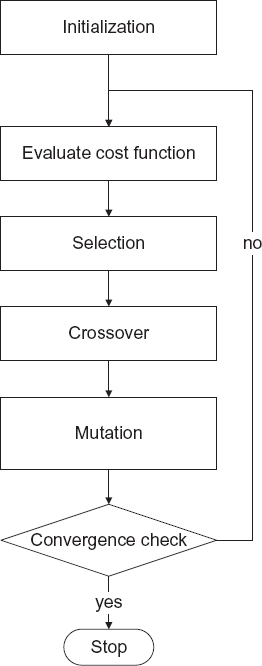
FIGURE 7.1 Flowchart of a basic genetic algorithm.
Crossover and Mutation. The selection phase is followed by the application of two genetic operators: crossover and mutation. The crossover operator combines two selected chromosomes and can be indicated as Ψkc = C(Ψka, Ψkb), where Ψka and Ψkb are two randomly selected chromosomes of the ![]() kS population. Application of the crossover operation results in a new population
kS population. Application of the crossover operation results in a new population ![]() kC = C(
kC = C(![]() kS).
kS).
The mutation operation acts on the elements of the ![]() kC population by perturbing the genes of the chromosomes of the population. The result of the mutation operation is a new population
kC population by perturbing the genes of the chromosomes of the population. The result of the mutation operation is a new population ![]() kM = M (
kM = M (![]() kC). At this point, the population of chromosomes obtained is used to start the process at the (k + 1)th iteration. In other words, the starting population at the (k + 1)th iteration can be viewed as a composed function
kC). At this point, the population of chromosomes obtained is used to start the process at the (k + 1)th iteration. In other words, the starting population at the (k + 1)th iteration can be viewed as a composed function ![]() k+1 = M{C[S(
k+1 = M{C[S(![]() kS)]} (Weile and Michielssen 1997).
kS)]} (Weile and Michielssen 1997).
Elitism. Often the so-called elitism operator is used. If Ψkq is the best chromosome at the kth iteration, that is, if ξkq = argmin {Fpk}, this chromosome is directly included in the new population ![]() k+1. In this way, the best solution is directly propagated into the next iteration.
k+1. In this way, the best solution is directly propagated into the next iteration.
The iterative process terminates when a given stopping criterion is fulfilled or when a prescribed maximum number of iterations is reached.
Concerning the possible selection strategies, the most widely used are the population decimation, the proportionate selection, and the tournament selection. In the population decimation (ranking selection), a fixed (arbitrary) maximum fitness is chosen as a cutoff. If Fkth denotes such a threshold values, the Q individuals with fitness such that Fkq < Fkth, q = 1,..., Q, are used to generate new individuals through pairing and reproduction. This deterministic procedure is very simple, but a given discarded individual can possess unique important characteristics (some genetic information) that could become important in successive stages of the optimization process. These characteristics are lost by using this selection scheme.
In the proportional selection, the population PkS is randomly constructed by selecting the individuals with a probability that is proportional to values of their cost functions. The selection probability for the qth element at the kth iteration is given by
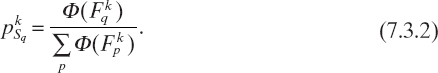
The function Φ is used to map the objective function to a non-negative interval such that, in minimization problems, low cost values correspond to high probabilities. Consequently, individuals with small cost have a high probability to be selected. This selection procedure is often called a roulette wheel, since an angular sector of a wheel (proportional to the fitness function) can be associated with each individual. Then the wheel is “spun” and the individual pointed at the end of the rotation is selected. Although the proportional selection is probably the most popular, it can result in a premature convergence if the chromosomes in a given population have very similar or very different fitness levels (Rahmat-Samii and Michielssen 1999). A possible solution is to use a fitness scaling to ensure that populations with many similar individuals do not tend to stagnate or that the best elements are not overrepresented in ![]() ks. The scaling approach requires that scaling values be calculated and checked at each iteration [e.g., in maximizing a function, since the proportional selections work only with positive values of the cost function, it must be ensured that negative scaled values are not obtained (Rahmat-Samii and Michielssen 1999)].
ks. The scaling approach requires that scaling values be calculated and checked at each iteration [e.g., in maximizing a function, since the proportional selections work only with positive values of the cost function, it must be ensured that negative scaled values are not obtained (Rahmat-Samii and Michielssen 1999)].
For these reasons, tournament selection is often preferred. In this selection strategy, a subset of R < Pk individuals is randomly selected from the original population (R is called tournament size). These elements “compete,” and the element with the best fitness wins the tournament and is selected for the subsequent stages of the process. The choice of R determines the selective pressure, and the tournament selection acts as an implicit fitness scaling. Sometimes, one assumes R = 2. It seems that the tournament selection behaves better than the proportional selection in the initial phases of the optimization. Moreover, by using the tournament selection, positive values of the fitness function are not required and the strategy can be simply used for example in minimization problems (Rahmat-Samii and Michielssen 1999).
Other strategies can be used, because of great flexibility offered by the genetic algorithm. For example, if one uses the tournament selection with R = 2, after the choice of the two chromosomes, it is possible to determine the new element of the population by using the Metropolis criterion [equation (7.2.1)]. In this way the genetic algorithm is simply hybridized with the simulated annealing, but it should be noted that the temperature becomes another parameter to control during the optimization process.
None of the previous selection strategies guarantees that the fittest individual of a given population will be reproduced in the new population. Consequently, usually the elitism strategy mentioned above is used.
Owing to the flexibility of the method, a plethora of different versions of the genetic algorithm can be implemented by simply changing the structures of chromosomes, operators, and so on (Haupt and Haupt 2004).
As far as the coding of chromosomes is concerned, in the simplest implementation, the chromosomes Ψkp are represented by strings of 0 and 1. Moreover, the crossover operator is defined as
![]()
![]()
where r is a random integer number uniformly distributed that determines the crossover point. The crossover operator is applied with a fixed probability pc, which represents one of the parameters of the method that can be chosen by the user.
Analogously, the mutation operation, in the binary coding, can be simply obtained by randomly changing one of the bits (genes) of the chromosome of the population ![]() kC (from 1 to 0 or from 0 to 1). All the chromosomes of the population are considered for mutation, but the mutation operation, too, is applied with a certain probability pm (usually much lower than pc).
kC (from 1 to 0 or from 0 to 1). All the chromosomes of the population are considered for mutation, but the mutation operation, too, is applied with a certain probability pm (usually much lower than pc).
The basic formulation of the genetic algorithm can be evidently improved by introducing extended versions of the genetic operators, as well as different selection and reproduction strategies. In-depth discussions about these improved versions can be found in the books listed in the reference section. However, since the encoding and decoding operations required by the binary-coded version of the genetic algorithm are computationally expensive, real-coded versions are now usually preferred. In these cases, the unknown parameters are not represented by a string of bits, but any real parameter is itself a gene of the chromosome (i.e., ξkp ≡ Ψkp for any p and k). Obviously, new definitions for the genetic operators are needed. In particular, concerning crossover and mutations, the simplest extensions of the previous definitions are
![]()
where q is a random value between 0 and 1, which is selected with a uniform probability. In the same way, the mutation can be simply obtained by adding random numbers to certain genes. In the real-coded version of the genetic algorithm, the mutation operator can be applied with a fixed probability pm.
Genetic algorithms are very helpful in solving highly constrained problems. Moreover, they are particularly suitable for applications in which the unknowns to be retrieved can create problems for deterministic methods and local search methods. From this perspective, they can be successfully applied to inverse problems in which there is significant information on the unknown target, but this information is difficult to factor in using local methods.
An example of application of the real-coded genetic algorithm is as follows. In particular, the reference configuration introduced in Chapter 5 is considered again (Fig. 5.1). The signal-to-noise ratio (SNR) is 25dB. The cost functional F is the discrete version of equation (6.7.1) with only the data term (6.7.2). In order to reduce the number of unknowns, spline basis functions have been used to discretize the scattering equations, following the approach in the study by Baussard et al. (2004). In this case, the number of unknowns (which are the coefficients of the splines) is 81. According to guidelines reported in the literature, the following parameters of the genetic algorithm have been chosen: Pk = P = 100 for any k, probability of crossover pc = 0.8, probability of mutation pm = 0.2, and threshold on the cost function Fth = 0.1. The maximum number of iterations kmax is 500. Figure 7.2 shows the reconstructed profile of the relative dielectric permittivity. As can be seen, the approach is able to correctly identify the scatterer. Figures 7.3 and 7.4 present the cost function values and the corresponding reconstruction errors (e) for the best individual of the population versus the iteration number, respectively.
A second example concerns a more complex situation, in which two separate lossless scatterers are present in the investigation domain. In particular, two circular cylinders of radius r = 0.25λ0 are located at (0.5λ0, 0.5λ0) and (−0.5λ0, 0). The dielectric characteristics of the two objects are ε1 = 1.6ε0 and ε1 = 1.4ε0, respectively.
The measured data are acquired by using a multiview configuration. In particular, S = 8 views are considered. At each view, the incident electric field is generated by a line-current source located at

and the scattered electric field is measured in M = 55 points, located at
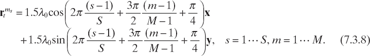
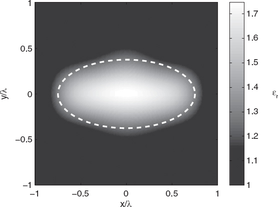
FIGURE 7.2 Reconstructed distribution of the relative dielectric permittivity of an elliptic cylinder (εr = 1.6); genetic algorithm.
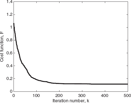
FIGURE 7.3 Reconstruction of an elliptic cylinder (Fig. 7.2). Cost function of the best individual of the population versus the iteration number; genetic algorithm.
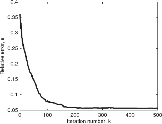
FIGURE 7.4 Reconstruction of an elliptic cylinder (Fig. 7.2). Relative reconstruction error of the best individual of the population versus the iteration number; genetic algorithm.
The electric field data (input data) are computed by using a direct solver based on the method of moments, which discretize the scene by means of N = 1681 pulse basis functions. Moreover, the computed values are corrupted with an additive Gaussian noise with zero mean value and a variance corresponding to a SNR of 25 dB.
As in the previous case, spline basis functions are used to discretize the inverse problem and the same parameters of the genetic algorithm are chosen. Figure 7.5 shows the reconstructed profile of the relative dielectric permittivity and proves that both the scatterers are correctly localized. Figures 7.6 and 7.7 present, for the best individual case, the cost function values and the related reconstruction errors.
The genetic algorithm has been proposed for solving several inverse problems related to microwave imaging. The key differences among the various approaches reported in the literature concern not only the adopted version of the genetic algorithm (mentioned previously) but also the inverse scattering formulation and the procedure used, at each iteration, for solving the direct scattering problem and computing the cost function.
From a historical perspective, one of the first applications of the genetic algorithm to inspect dielectric bodies was reported by Kent and Gunel (1997), who reconstructed two-layer dielectric cylinders. In particular, they assumed the outer radii of the cylinders to be known, and formed the chromosomes by binary-coding the values of the dielectric permittivities of the materials constituting the two layers as well as the value of the internal radius. They used 7 bits for any unknown parameter. This represents an example in which some a priori information on the scatterers under test (the external shape) is directly included into the model. The simulations that they reported assumed a plane-wave transverse magnetic illumination at a frequency f = 3 GHz, and the scattered data were collected on a linear probing line whose distance from the center of the cylinder was equal to 10λ with measurements performed on 64 points equally spaced at λ/4.
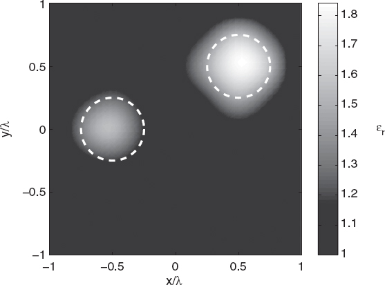
FIGURE 7.5 Reconstructed distribution of the relative dielectric permittivity of two circular cylinders, calculated using the genetic algorithm.
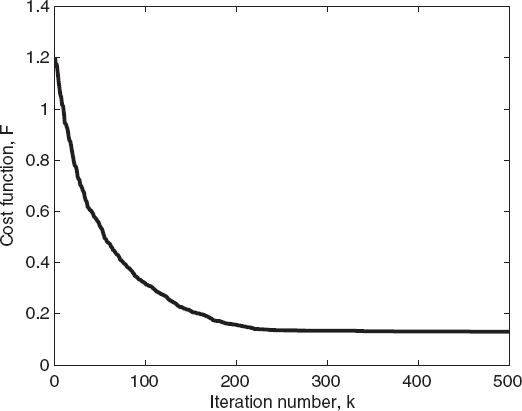
FIGURE 7.6 Reconstruction of two circular cylinders (Fig. 7.5). Cost function of the best individual of the population versus the iteration number, calculated using the genetic algorithm.
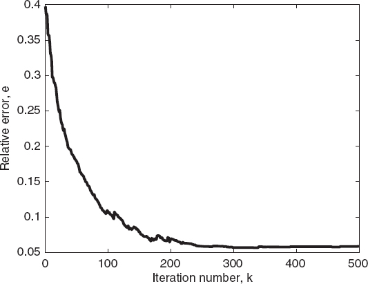
FIGURE 7.7 Relative reconstruction error of the best individual of the population versus the iteration number (two circular cylinders), calculated using the genetic algorithm.
For this very simple application, the cost function [equation (6.7.1)] was constituted only by the data term [equation (6.7.2)] and the forward computation, at each iteration of the genetic algorithm, was performed analytically. Moreover, the cylinders under test had relatively small dielectric permittivities (εr ≤ 1.5), which have been searched in the range 1.0 ≤ εr ≤ 2.0. It should be noted that the ability of the approach in reducing the search space has been exploited. The accuracy of the reconstructions has been of course very good since a reduced parameterization and noiseless input data have been used. The binary-coded genetic algorithms has been successively applied in several other cases. A significant example is the retrieval of the external shape of PEC cylinders. To inspect PEC cylinders, according to the formulation described in Section 3.3, the shape of the object is defined by a shape function ρ(φ) (in cylindrical coordinates), which defines a closed curve (the profile of the infinite cylinder is a closed line in the transversal plane). A common representation concerns the expansion in trigonometric series as

where the coefficients An and Bn are now the unknowns to be retrieved. Chiu and Liu (1996) applied a binary genetic algorithm to recover these parameters. In the construction of the function, a regularization term (see Section 6.7) given by P = α|ρ′(φ)|2 has been added to the data term, and the regularization parameter α (heuristically determined) essentially depends on the problem dimensions [0.0001 < α < 10 (Chiu and Liu 1996)]. The imaging configuration contained 32 measurement points equally spaced on a circumference of radius 10λ, whereas the scatterer cross section was illuminated by a set of eight plane waves with different incident angles. The binary chromosomes have been constructed by using 8 bits for each parameter, and the nine coefficients of equation (7.3.9) have been considered for reconstructing simple scatterers with contours represented by smooth functions, suitable for trigonometric representations. The crossover and mutation probabilities were pc = 0.8 and pm = 0.04, respectively, and the population consisted of P = 300 elements. Quite good results have been obtained for cylindrical objects with maximum transversal dimensions slightly exceeding one wavelength starting from simulated input data numerically corrupted by Gaussian noise with zero mean values and standard deviations (normalized to the square amplitude of the simulated scattered values) σn ≤ 0.4.
This work has been successively extended to inspect different dielectric and conducting cylinders in order to evaluate the capabilities and limitations of the genetic algorithm. Some examples are mentioned. Homogeneous dielectric cylinders with finite electrical conductivities have been reconstructed (Chiu and Chen 2000), whereas other PEC cylinders partially immersed in a homogeneous half-space (Fig. 4.8) (Yang and Chiu 2002) or located inside a multilayer material (Lin et al. 2004) have been inspected. The studies above cited have provided some further indications concerning the application of binary-coded genetic algorithms to microwave imaging. In particular, good results have been obtained by using a population of about 300–600 individuals, in which any parameter has been coded by means of 8–16 bits, whereas the crossover probability and mutation probability have been chosen in the ranges 0.5–0.7 and 0.005–0.05, respectively.
Qualitative inverse scattering formulations have also been used in conjunction with the genetic algorithm in order to inspect inhomogeneous dielectric cylinders of arbitrary shapes under transverse magnetic (TM) illumination conditions. The first-order Born approximation [see Section 4.6 and equation (4.6.7)] has been applied (Caorsi and Pastorino 2000), and the second-order Born approximation [see Section 4.6, where the solving equation is the two-dimensional counterpart of equation (4.6.6)] has also been considered (Caorsi et al. 2001). However, it is worth mentioning that the very high computational load associated with stochastic optimization procedures leaves the reconstruction of pixelated images of inhomogeneous targets still a very challenging problem.
Despite the interesting results obtained by using binary-coded genetic algorithms, real-coded versions of the method have been applied more frequently. For example, the external contours of arbitrarily shaped PEC cylinders have been retrieved (Qing and Zhong 1998, Qing and Lee 1999; Qing et al. 2001). These contours have been represented by equation (7.3.9), but the unknown coefficients An and Bn directly formed the chromosomes [nine real elements used by Qing et al. (2001)]. The suggested parameters for the genetic algorithm application were crossover and mutation probabilities: pc = 1.0 and pm = 0.04, respectively, whereas the population was composed of P = 300 elements. The cost function was constituted by the data term only.
The reconstruction capabilities of the real-coded genetic algorithm can be drawn by the example presented in Figure 7.8, which shows the reconstruction, starting from noiseless data, of a single PEC cylinder whose contour is represented by the equation
![]()
In particular, Figure 7.8a shows the original and estimated contours. It should be noted that initial contour is very different from the original one. Nevertheless, the final reconstruction is almost perfect. The genetic algorithm, as well as other evolutionary algorithms, does not require that the initial solution be close to the exact one. The behavior of the cost function, for the same simulation, is shown in Figure 7.8b.
Another application for which the genetic algorithm has been proposed is the determination of the widths and positions of strips located in a given investigation region (Takenaka et al. 1998). For a two-dimensional geometry, the metallic strip may be located along a certain line. This line can be discretized in small segments, and each segment may or may not belong to a strip. This problem is essentially a binary problem, in which a shape function is associated with the line where the strips are present. In particular, for each segment of the line, the shape function is equal to 1 if the segment is occupied by the metal strip, and 0 in the other case. By using a surface scattering formulation, the measured scattered electric field can be expressed in terms of this shape function. This approach has been considered in the study by Takenaka et al. (1998), where the scattering of a series of separated objects was computed by using an additional theorem (Chew 1990). However, the related inverse problem has been recast as an optimization problem by using a single cost function term, and the binary nature of the problem has been exploited. In particular, as the shape function is the only problem unknown, the inverse problem has been solved by using a standard binary genetic algorithm. It should be observed that this formulation implies a straightforward extension to two-dimensional configurations. In particular, the reconstruction of a two-dimensional configuration of small cylinders of square cross sections has also been reported (Takenaka et al. 1998).
Some examples of the different implementations of the genetic algorithms can be mentioned. Nonuniform probability densities for the genetic operators of a binary-coded genetic algorithm have been used (Chien and Chiu 2003) for the reconstruction of dissipative dielectric cylinders, and “start and restart” procedures have been applied as well. In the latter case, the genetic algorithm is applied with a very small population. The approach reaches the near-optimal region of the solution space by a repeated computation. This version of the stochastic procedure, called the micro genetic algorithm (micro-GA) (Krishnakumar 1989), has been applied for reconstruction of the contours of PEC cylinders (Xiao and Yabe 1998; Huang and Mohan 2004). As an example, the approach in the study by Xiao and Yabe (1998) was a binary-coded version that uses a population composed by five elements only.
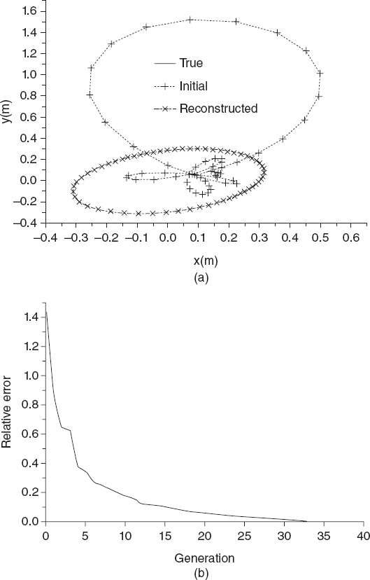
FIGURE 7.8 Reconstruction of a single PEC cylinder with the shape function of equation (7.3.10), using the genetic algorithm: (a) plots of the contours of the cross section at different iterations; (b) cost function (error function) versus the iteration number. [Reproduced from A. Qing, C. K. Lee, and L. Jen, “Electromagnetic inverse scattering of two-dimensional perfectly conducting objects by real-coded genetic algorithm,” IEEE Trans. Geosci. Remote Sens. 39(3), 665–674 (March 2001), © 2001 IEEE.]
Some other ideas on implementation of the genetic algorithms have been exploited in implementing codes for microwave imaging applications. For example, application of a parabolic form of the crossover operator has been proposed (Bort et al. 2005) and, since the same trial solutions can be repeatedly considered during the optimization approach, the use of a so-called tabu list has been proposed in conjunction with standard genetic algorithms for the detection of metallic objects with cavities (Zhou et al. 2003).
7.4 THE DIFFERENTIAL EVOLUTION ALGORITHM
The differential evolution algorithm (Storm and Price 1997; Chakraborty 2008) is a more recently proposed stochastic optimization method. A flowchart of this algorithm is shown in Figure 7.9.
The overall structure of the differential evolution algorithm is similar to those of the GA. The differential evolution algorithm iteratively modifies a population ![]() k of Pk elements, ξkp, p = 1,..., Pk, where k is the iteration number. Usually, the number of elements in the population does not change during the evolution of the algorithm and the trial solutions are real-coded: ξkp → Ψkp = [ψkp1, ψkp2,..., ψkpn,..., ψkPN] [equation (7.3.1)], with ψkpn ∈
k of Pk elements, ξkp, p = 1,..., Pk, where k is the iteration number. Usually, the number of elements in the population does not change during the evolution of the algorithm and the trial solutions are real-coded: ξkp → Ψkp = [ψkp1, ψkp2,..., ψkpn,..., ψkPN] [equation (7.3.1)], with ψkpn ∈ ![]() . As is the genetic algorithm, the differential evolution algorithm is based on genetic operators. The main difference, however, relies on the scheme used for generation of the offspring. In particular, all the trial solutions are used once and in a deterministic way as parents to producing offspring. This property ensures a good exploration of the search space. A schematic representation of the offspring generation process is shown in Figure 7.10, and the steps in the algorithm are briefly described as follows:
. As is the genetic algorithm, the differential evolution algorithm is based on genetic operators. The main difference, however, relies on the scheme used for generation of the offspring. In particular, all the trial solutions are used once and in a deterministic way as parents to producing offspring. This property ensures a good exploration of the search space. A schematic representation of the offspring generation process is shown in Figure 7.10, and the steps in the algorithm are briefly described as follows:
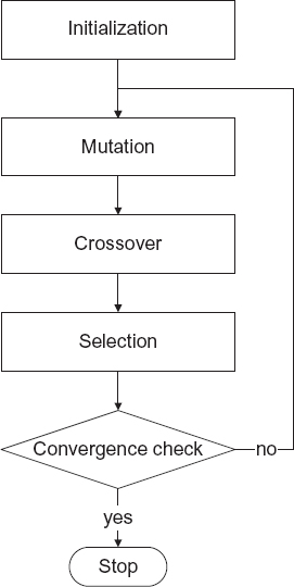
FIGURE 7.9 Flowchart of differential evolution algorithm.
Initialization. In the initialization phase, the starting population of the differential evolution algorithm can be constructed by randomly creating P0 arrays of N real values:
![]()
where Ψn,L and Ψn,U are the lower and upper bounds of the nth component of the elements of the population, respectively. In the same equation, rand(0,1) is a function that returns a random number uniformly distributed in the range [0,1]. Clearly, it is possible to introduce some a priori information in the initialization phase by properly modifying equation (7.4.1). Moreover, it is evident that the comments made in Section 7.3 about the possibility of including a priori information into the model are still valid here.
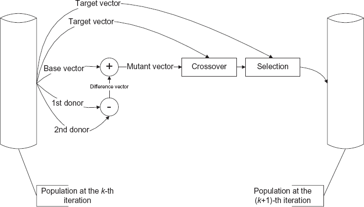
FIGURE 7.10 Schematic representation of the offspring generation in the differential evolution algorithm.
Mutation. In the differential evolution algorithm, the first applied operator is the mutation, which generates a set of Pk new elements. In particular, a new trial solution Vkp is generated by perturbing an element of the population (called a base vector) by using a difference-based mutation. In the literature, several different versions of the mutation operators have been proposed, which differ mainly in the strategy of selection of the base vectors and in the number of difference vectors used (Chakraborty 2008). The various types of strategies are usually identified by the notation DE/x/y/z (Storn and Price 1997), where x denotes the base vector selection strategy, y is the number of difference vectors, and z indicates the type of crossover (the last point will be discussed later). As an example, in the DE/rand/1/* variant, the base vector is chosen randomly in the current population and only one difference vector is used to mutate it:
![]()
Here, cf is a weighting factor that controls the amplification of the difference array, and p0, p1, and p2 are randomly selected indices, which identify the base vector and the two elements used to generate the difference array, respectively. The reader is referred to the text by Chakraborty (2008) for an overview of the various mutation operators developed in the framework of differential evolution algorithms. It is worth noting that the mutant vector is generated by using only randomly chosen elements of the population, which allows one to account for the population diversity and limit the destructive effect of the mutation operator.
Crossover. Crossover works on the arrays generated in the mutation stage and on the elements Ψkp of the current population (which, in the crossover stage, are called target vectors) in order to generate a set of trial vectors Ukp. Analogously to the mutation operator, several variants of crossover have been proposed in the literature (Storn and Price 1997). A crossover operator commonly used is the uniform crossover, defined as

where j is a random integer selected in [0, N], ukpn and vkpn are the nth components of the arrays Ukp and Vkp, respectively, and cr is the crossover rate.
Selection. In the differential evolution algorithm, the pth element of the population at the (k + 1)th iteration is generated from the trial and target vectors by using a simple one-to-one survivor selection:
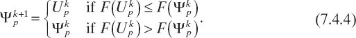
As in the genetic algorithm, the procedure stops when a given stopping criterion is fulfilled or when a prescribed maximum number of iterations, kmax, is reached.
The choice of the values of the control parameters, cf and cr, is essentially heuristic and related to the particular problem in which the differential evolution is used. However, some general suggestions are provided in the literature (Chakraborty 2008, Price et al. 2005). In particular, cf is usually chosen in the range [0.5, 1.0], and the value of cr in the range [0.8, 1.0]. If the parameters cr and cf are suitably chosen, a good balance between good convergence speed and low possibility of a premature convergence to local minima can be obtained.
It is worth noting that the differential evolution algorithm contains a kind of implicit elitism. In fact, since the fitness of the trial vector Ukp is compared only with the one of the target vector Ψkp from which it is generated, the corresponding element in the next generation has a fitness that can only be better than or at least equal to the one of Ψkp.
In order to reduce the computational load, application of the differential evolution to imaging problems requires a reduced parameterization. Michalski (2000, 2001) obtained this by approximating the cylindrical scatterers with canonical objects with circular and elliptic cross sections. The proposed application concerns the inspection of tunnels and pipes in a cross-borehole configuration (Michalski 2001), in which the effects of the interface between the upper and lower media were neglected assuming deeply buried objects. In the inverse problem, the problem unknowns are represented by the cylinder center and the radius (circular cross section) or the semimajor axis, the eccentricity, and the tilt angle (elliptic cross section). The differential evolution algorithm has been applied to a cost function based on the data equation only [equation (6.7.2)]. Excellent reconstructions have been obtained with the following control parameters: P = 25, kmax = 40 (maximum number of iterations of the differential evolution), cr = 0.9 and cf = 0.7.
Massa et al. (2004) applied the differential evolution algorithm by combining two of the various possible implementation strategies for this evolutionary approach. In particular, the DE/1/best/bin version (Storn and Price 1997) is used until the cost function has reached a predefined value; successively, the DE/1/rand/bin strategy (Storn and Price 1997) is applied. It has been found that the DE/1/best/bin strategy is quite able to rapidly locate the attraction basin of a minimum, but, since it uses the best individual of the population to perform the mutation, it can sometimes be trapped in a local minimum. This drawback is overcome by switching, after a predefined threshold, to the DE/1/rand/bin strategy, which is able to explore more efficiently the search space, without modifying the previous best solution if it is inside the correct attraction basin. Concerning the choice of the control parameters, cf has been chosen in the range [0.5, 1.0], whereas good reconstructions have been obtained with cr = 0.8.
The differential evolution algorithm has been further applied to inspect single and multiple PEC cylinders of arbitrary shapes (Qing 2003, 2006). The approach has been successfully used to obtain good reconstructions of the profiles of PEC cylinders (with both synthetic and real data) by using the following values of control parameters: cr = 0.9 and cf = 0.7. For this specific application, the differential evolution method has been compared with a standard real-coded genetic algorithm under the same operating conditions. In this case, the differential evolution algorithm has been found to outperform the genetic algorithm, due to the need for a smaller population. It should be mentioned that in Qing (2006) used the dynamic differential evolution strategy, in which an additional competition is introduced between the trial vector and the current optimal individual. The current optimal element is replaced if the new element corresponds to a better solution and the updated element is immediately included in the new population.
In an example application of the differential evolution, the reference configuration is the same as in Section 7.3 (Fig. 7.2). The parameters of the differential evolution algorithm are P = 100, kmax = 500, Fth = 0.1, cr = 0.8, and cf is randomly chosen in the range [0.5, 1.0]. In this example, the DE/rand/1/bin strategy (Storn and Price 1997) is applied. The same cost function [equation (6.7.2)] and the same spline basis functions (Baussard et al. 2004) are also used. Figure 7.11 shows the reconstructed distribution of the relative dielectric permittivity of the investigation area obtained by the differential evolution algorithm. Figures 7.12 and 7.13 plot the behavior of the cost function and the relative reconstruction errors (related to the best individual of the population) versus the iteration number, respectively. As can be seen from these figures, the approach correctly reconstructs the shape and dielectric properties of the scatterer.
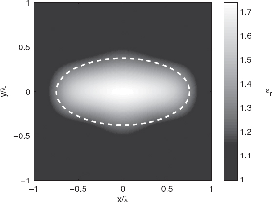
FIGURE 7.11 Reconstructed distribution of relative dielectric permittivity of an elliptic cylinder, calculated using the differential evolution algorithm.
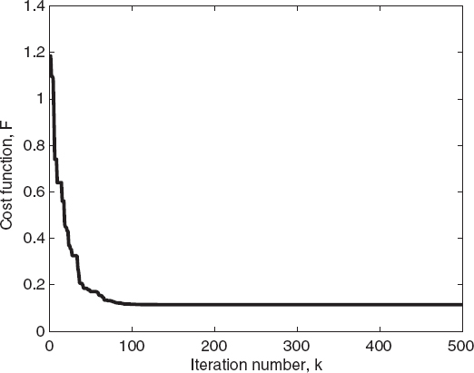
FIGURE 7.12 Cost function of the best individual of the population versus the iteration number calculated for an elliptic cylinder using the differential evolution algorithm.
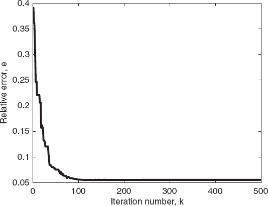
FIGURE 7.13 Relative reconstruction error of the best individual of the population versus the iteration number for an elliptic cylinder, calculated using the differential evolution algorithm.
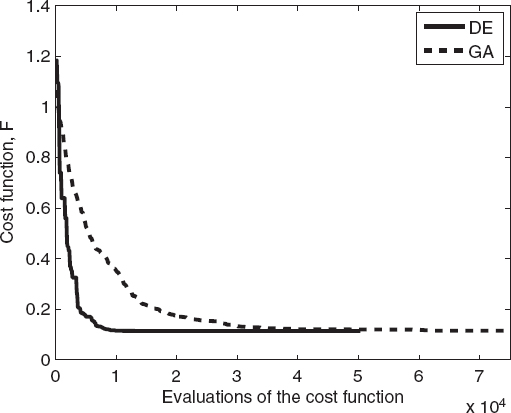
FIGURE 7.14 Comparison between the differential evolution algorithm and the genetic algorithm for calculation of cost function value versus number of cost function evaluations for an elliptic cylinder.
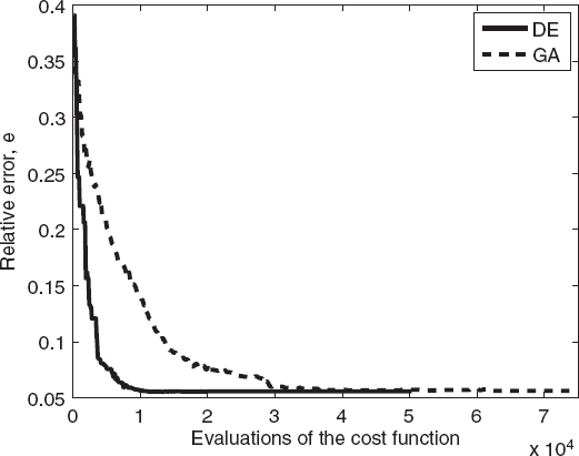
FIGURE 7.15 Comparison between the differential evolution algorithm and the genetic algorithm for estimating relative reconstruction error versus number of cost function evaluations for an elliptic cylinder.

FIGURE 7.16. Reconstructed distribution of the relative dielectric permittivity of two circular cylinders, calculated using the differential evolution algorithm.
Moreover, as can be seen from Figure 7.12, the differential evolution algorithm converges more rapidly than does the genetic algorithm. This behavior can be better evaluated from Figures 7.14 and 7.15, which provide a direct comparison in terms of the cost function values and of the relative errors for the best individual of the population. For the present case, the differential evolution algorithm requires fewer cost function evaluations than does the standard genetic algorithm to reach the final solution.
As a second example, the configuration adopted in Section 7.3 for the reconstruction shown in Figure 7.5 is considered. The parameters of the differential evolution are P = 100, kmax = 500, Fth = 0.1, and cr = 0.8, and cf is randomly chosen in the range [0.5, 1.0]. The DE/rand/1/bin strategy (Storn and Price 1997) is employed. Figure 7.16 shows the distribution of the reconstructed relative dielectric permittivity obtained by applying the differential evolution method. Figures 7.17 and 7.18 give the plots of the cost function and of the corresponding reconstruction errors. As can be seen, in this case, too, the differential evolution algorithm converges faster than does the genetic algorithm.
7.5 PARTICLE SWARM OPTIMIZATION
Particle swarm optimization is another global optimization algorithm, which is inspired by the social behavior of bird flocking or fish schooling (Kennedy and Eberhart 1995, 1999; Robinson and Rahmat-Samii 2004). Similarly to other evolutionary computation techniques, it is based on a population (swarm) of trial solutions (particles), which is iteratively updated by following a predefined set of rules. Unlike other approaches, however, particle swarm optimization does not rely on evolution operators, but modifications are introduced in order to follow the current best solutions. One of the main advantages of particle swarm optimization, with respect to other techniques such as the genetic algorithm is that it is simple to implement and requires adjustment of only a few parameters. Moreover, a priori information can be easily inserted into the updating scheme. Finally, particle swarm optimization generally requires a rather small population size, which results in a reduced computational cost of the overall minimization process (Clerk and Kennedy 2002, Robinson and Rahmat-Samii 2004).
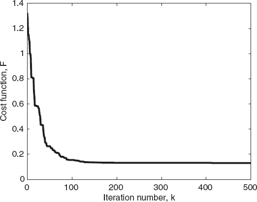
FIGURE 7.17 Cost function of the best individual of the population versus the iteration number for two circular cylinders, estimated using the differential evolution algorithm.
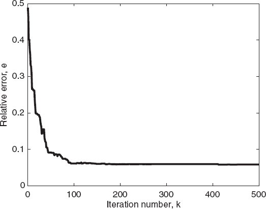
FIGURE 7.18 Relative reconstruction error of the best individual of the population versus the iteration number for two circular cylinders, calculated using the differential evolution algorithm.
In order to describe how particle swarm optimization works, let us consider a population ![]() k of P elements, ξkp, p = 1,..., P (as usual, k is the iteration number). Let us suppose that the elements are again real-coded, ξkp → Ψkp = [ψkp1, ψkp2,..., ψkpn,...,ψkPN] [equation (7.3.1)], with ψkpn ∈
k of P elements, ξkp, p = 1,..., P (as usual, k is the iteration number). Let us suppose that the elements are again real-coded, ξkp → Ψkp = [ψkp1, ψkp2,..., ψkpn,...,ψkPN] [equation (7.3.1)], with ψkpn ∈ ![]() . In the particle swarm optimization framework, ξkp is usually referred to as the position of the pth particle of the swarm. Moreover, a velocity vector Vkp = [νkp1, νkp2,...,νkpn,...,νkPN] is associated with each trial solution of the population.
. In the particle swarm optimization framework, ξkp is usually referred to as the position of the pth particle of the swarm. Moreover, a velocity vector Vkp = [νkp1, νkp2,...,νkpn,...,νkPN] is associated with each trial solution of the population.
Particle swarm optimization is characterized by the following steps:
Initialization. When no a priori information is available, the particle population is initialized with randomly chosen values.
Swarm Ranking. At each iteration, the cost function values of the particles are evaluated, and two “best” solutions are identified. The first one, Pbest = [pbest1, pbest2,..., pbestn,..., pbestN], is the best solution achieved so far by a given particle (i.e., by the pth element of the population). The second one, Gbest = [gbest1, gbest2,..., gbestn,..., gbestN], is the “best” value obtained so far by any particle of the population (i.e., it is a global “best”).
Solution Update. At each iteration, both the elements ξkp (positions of the particles) and the velocity vectors Vkp are updated. In particular, the following rules are used to construct the ![]() k+1 population:
k+1 population:

![]()
Here, r1 and r2 are random numbers uniformly distributed in the range [0, 1], c1 and c2 are positive constants called acceleration coefficients (usually chosen such that c1 = c2 = 2), and w is a scaling factor. Usually, the velocities of the particles are also clamped to a maximum value νmax. The algorithm stops when a suitable stopping criterion is satisfied. A high-level pseudocode of the particle swarm optimization method is presented in Figure 7.19.
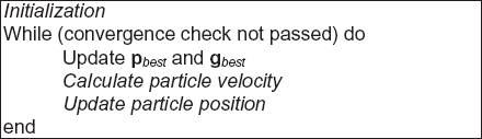
FIGURE 7.19 Particle swarm optimization algorithm.
The differential evolution method has been shown to outperform the particle swarm optimization method in reconstructing perfectly conducting scatterers limitedly to the specific cases considered (Rekanos 2008). The reader is also referred to studies by Donelli et al. (2006), Donelli and Massa (2005), and Huang and Mohan (2005, 2007) for further details on particle swarm optimization.
7.6 ANT COLONY OPTIMIZATION
The ant colony optimization method is a more recently introduced stochastic optimization algorithm, which was originally inspired by the way ants find the optimal path from nest to food (Dorigo and Gambardella 1997, Dorigo et al. 2006). By exploiting these ideas, the ant colony optimization method was initially developed to solve difficult combinatorial problems, such as the “traveling salesperson” problem but has more recently been extended to continuous domains (Socha and Dorigo 2008).
The ant colony optimization algorithm performs the minimization of a cost function F by iteratively modifying a population ![]() k of P trial solutions, ξkp, p = 1,..., P, where k is the iteration number. In the continuous version of ant colony optimization, the elements of the population are real-coded: ξkp → Ψkp = [ψkp1, ψkp2,..., ψkpn,..., ψkPN], with ψkpn ∈
k of P trial solutions, ξkp, p = 1,..., P, where k is the iteration number. In the continuous version of ant colony optimization, the elements of the population are real-coded: ξkp → Ψkp = [ψkp1, ψkp2,..., ψkpn,..., ψkPN], with ψkpn ∈ ![]() . The population is stored in an ordered archive: F (ξk1) ≤ F (ξk2) ≤ ... ≤ F (ξkp).
. The population is stored in an ordered archive: F (ξk1) ≤ F (ξk2) ≤ ... ≤ F (ξkp).
A high-level pseudocode of the ant colony optimization algorithm is shown in Figure 7.20.
The algorithmic steps shown in Figure 7.20 work as follows:
Initialization. An initial set of P randomly chosen trial solutions Ψ0p, i = 1,..., P, is constructed. In particular, when no a priori information is available, the components of Ψ0p are obtained by sampling a uniform probability density function (PDF) as in equation (7.4.1).
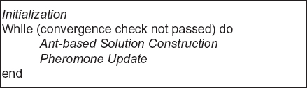
FIGURE 7.20 Ant colony optimization algorithm.
Ant-Based Solution Construction. At each iteration, a set of Q new trial solutions is created. The N components of the new solution are obtained by sampling a set of N Gaussian kernel PDFs (Socha and Dorigo 2008, Brignone et al. 2008a, 2008b), defined as

where mkpn, Skpn, and wP, p = 1,..., P, n = 1,..., N are parameters of the PDFs, which, at the kth iteration, are given by
![]()


where ξ (called the pheromone evaporation rate) and q are parameters of the ant colony optimization algorithm.
Pheromone Update. The new population ![]() k+1 is obtained by adding the newly created trial solutions to the ones contained in the current population
k+1 is obtained by adding the newly created trial solutions to the ones contained in the current population ![]() k and by discarding the worst Q elements. The algorithm stops when a maximum number of iterations is reached, or when a given stopping criterion is satisfied.
k and by discarding the worst Q elements. The algorithm stops when a maximum number of iterations is reached, or when a given stopping criterion is satisfied.
An example application of the ant colony optimization algorithm is described as follows. In particular, the reference configuration introduced in Figure 5.1 is considered. Similarly to the case reported in Section 7.3, the scattering equations are discretized by using the method of moments with spline basis functions and Dirac delta distributions as testing functions. The population elements are the coefficients of the spline expansion of the object function. The cost function considered is the same as that used in Section 7.3 (data equation only). The parameters of the ant colony optimization algorithm are P = 100, Q = 10, q = 0.1, ξ = 0.65, and kmax = 500. The algorithm stops when F(ξkp)≤ Fth, with Fth = 0.1 or when k > kmax. Figure 7.21 shows the reconstructed distribution of the relative dielectric permittivity.

FIGURE 7.21 Reconstructed distribution of the relative dielectric permittivity of an elliptic cylinder, calculated using the ant colony optimization algorithm.
Figures 7.22 and 7.23 plot the behavior of the cost function and the reconstruction errors versus the iteration number for the best element of each population. Figures 7.24 and 7.25 compare the ant colony optimization and differential evolution algorithms in terms of cost function values (Fig. 7.24) and relative reconstruction errors (Fig. 7.25) versus the number of evaluations of the functional. As can be seen, the ant colony optimization algorithm requires about half of the cost functional evaluations needed for the differential evolution method, resulting in a significant reduction in the computation time needed to perform the reconstruction.
The second reported example concerns the reconstruction of the two-cylinder configuration used in Section 7.3 to obtain Figure 7.5. The parameters of the ant colony optimization algorithm are P = 100, Q = 10, q = 0.1, ξ = 0.65, and kmax = 1000. The cost function is still the same as that used in the previous examples (data term only). Figure 7.26 shows the reconstructed distribution of the relative dielectric permittivity, whereas Figures 7.27 and 7.28 present the corresponding behaviors of the cost function and reconstruction errors calculated for the best individual of the population. Finally, Figures 7.29 and 7.30 compare the ant colony optimization and the genetic algorithms in terms of the number of evaluations. As can be seen, although it cannot be considered a general result, for this specific case, the ant colony optimization algorithm outperforms the standard genetic algorithm since it is able to reach the final solution with fewer cost function evaluations.
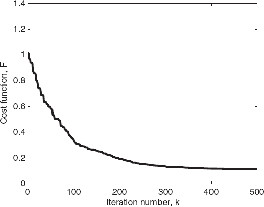
FIGURE 7.22 Cost function of the best individual of the population versus the iteration number for an elliptic cylinder, calculated using the ant colony optimization algorithm.
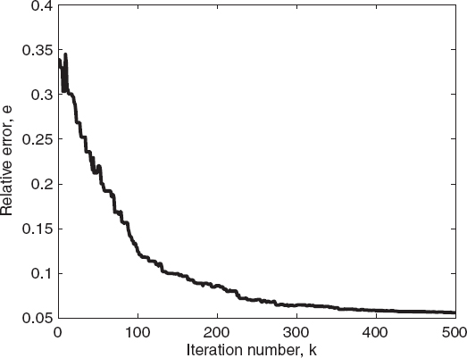
FIGURE 7.23 Relative reconstruction error of the best individual of the population versus the iteration number for an elliptic cylinder, calculated by the ant colony optimization algorithm.
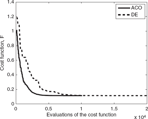
FIGURE 7.24 Comparison between ant colony optimization and differential evolution algorithms, showing cost function values (best individual) versus the number of evaluations of the functional for an elliptic cylinder.
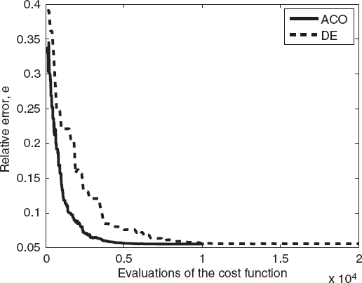
FIGURE 7.25 Comparison between the ant colony optimization and differential evolution algorithms, showing relative reconstruction errors (best individual) versus the number of evaluations of the functional for an elliptic cylinder.
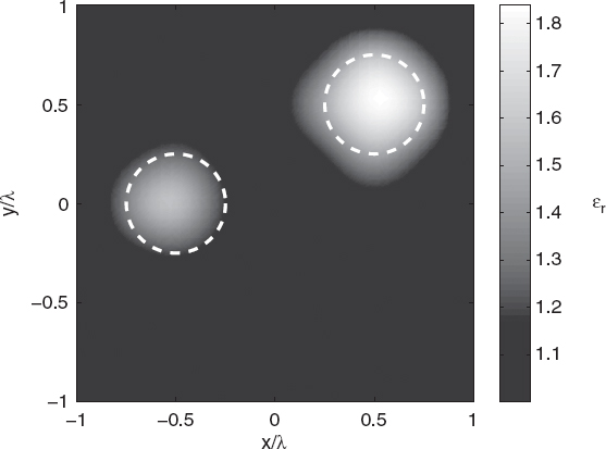
FIGURE 7.26 Reconstructed distribution of the relative dielectric permittivity of two circular cylinders, using the ant colony optimization algorithm.
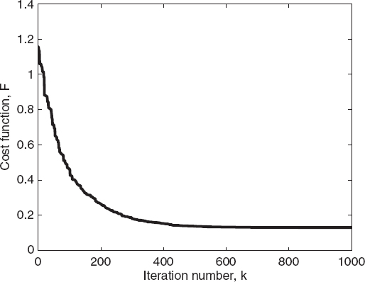
FIGURE 7.27 Cost function of the best individual of the population versus the iteration number for two circular cylinders, calculated using the ant colony optimization algorithm.
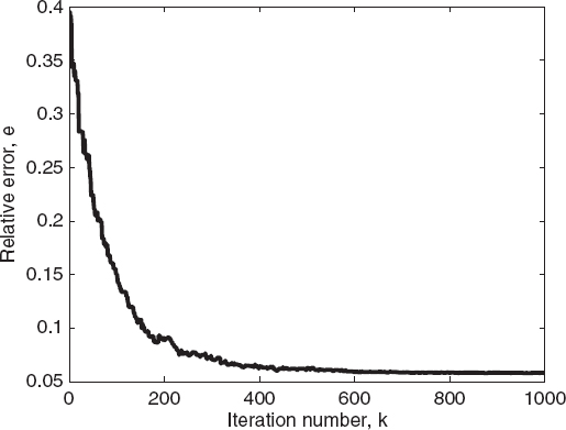
FIGURE 7.28 Relative reconstruction errors of the best individual of the population versus the iteration number for two circular cylinders, calculated using the ant colony optimization algorithm.
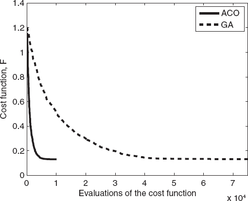
FIGURE 7.29 Comparison between the genetic algorithm and the ant colony optimization algorithm for calculation of cost function values of the best individual versus the number of the evaluations of the functional for two circular cylinders.
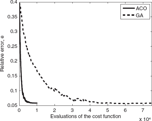
FIGURE 7.30 Comparison between the genetic algorithm and the ant colony optimization algorithm for estimation of relative reconstruction errors of the best individual versus the number of the evaluations of the functional for two circular cylinders.
7.7 CODE PARALLELIZATION
The application of stochastic optimization methods to solve the inverse scattering problem following the formulation described in the previous sections usually results in very expensive computational codes.
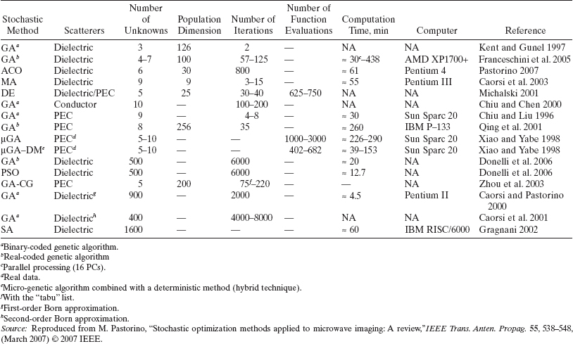
To give the reader an idea of the computational load, in a previous study (Pastorino 2007) the author provided data on some stochastic optimization approaches, even though they refer to very different configurations and parameterizations that do not allow for a direct comparison. Such data are presented in Table 7.1 and also pertain to some hybrid techniques, which are described in Chapter 8.
However, when possible, the computation time of the iterative reconstruction can be drastically reduced by using parallel processing. In fact, it is evident that the procedures discussed in Section 7.3–7.6 are intrinsically parallel algorithms since the various operators act on sets of solutions. Consequently, these operators can be applied simultaneously on different chromosomes of the population if more than one processor is available. Moreover, at the kth iteration step, computation of the values of the cost function Fkp = F (ξkp), which must be obtained for every chromosome Ψkp, must be parallelized as well. This results in another significant time saving. Discussion of the parallelization of computer codes is beyond the scope of present book; however, it is well known that the use of multiprocessor computers is now quite common and the availability of parallel systems is becoming increasingly widespread.
TABLE 7.1 Some Computational Data on Microwave Imaging Methods Based on Stochastic Optimization Algorithms
REFERENCES
Aarts, E. and J. Korst, Simulated Annealing and Boltzmann Machines, Wiley, New York, 1990.
Baussard, A., E. L. Miller, and D. Premel, “Adaptive B-spline scheme for solving an inverse scattering problem,” Inverse. Problems. 20, 347–365 (2004).
Bort, E., G. Franceschini, A. Massa, and P. Rocca, “Improving the effectiveness of GA-based approaches to microwave imaging through an innovative parabolic crossover,” IEEE Anten. Wireless Propag. Lett. 4, 138–142 (2005).
Brignone, M., G. Bozza, A. Randazzo, R. Aramini, M. Piana, and M. Pastorino, “Hybrid approach to the inverse scattering problem by using ant colony optimization and no-sampling linear sampling,” proc. 2008 IEEE Antennas Propagation. Society Int. Symp., San Diego, CA, July 5–11, 2008, pp. 1–4 (2008a).
Brignone, M., G. Bozza, A. Randazzo, M. Piana, and M. Pastorino, “A hybrid approach to 3D microwave imaging by using linear sampling and ACO,” IEEE Trans. Anten. Propag. 56, 3224–3232 (2008b).
Caorsi, S., A. Costa, and M. Pastorino, “Microwave imaging within the second-order Born approximation: Stochastic optimization by a genetic algorithm,” IEEE Trans. Anten. Propag. 49, 22–31 (2001).
Caorsi, S., G. L. Gragnani, S. Medicina, M. Pastorino, and G. Zunino, “Microwave imaging method using a simulated annealing approach,” IEEE Microwave Guided Wave Lett. 1, 331–333 (1991).
Caorsi, S., G. L. Gragnani, S. Medicina, M. Pastorino, and G. Zunino, “Microwave imaging based on a Markov random field model,” IEEE Trans. Anten. Propag. 42, 293–303 (1994).
Caorsi, S. and M. Pastorino, “Two-dimensional microwave imaging approach based on a genetic algorithm,” IEEE Trans. Anten. Propag. 48, 370–373, (2000).
Caorsi, S., M. Pastorino, M. Raffetto, and A. Randazzo, “Electromagnetic detection of buried inhomogeneous elliptic cylinders by a memetic algorithm,” IEEE Trans. Anten. Propagat. 51, 2878–2884 (2003).
Chakraborty, U. K., Advances in Differential Evolution, Springer, 2008.
Chew, W. C. Waves and Fields in Inhomogeneous Media, Van Nostrand Reinhold, New York, 1990.
Chien, W. and C.-C. Chiu, “Using NU-SSGA to reduce the searching time in inverse problem of a buried metallic object,” IEEE Trans. Anten. Propag. 53, 3128–3134 (2003).
Chiu, C.-C. and W.-T Chen, “Electromagnetic imaging for an imperfectly conducting cylinder by the genetic algorithm,” IEEE Trans. Microwave Theory Tech. 48, 1901–1905 (2000).
Chiu, C.-C. and P. T. Liu, “Image reconstruction of a perfectly conducting cylinder by the genetic algorithm,” IEE Proc. Microwaves Anten. Propag. 143, 249–253 (1996).
Clerk, M. and J. Kennedy, “The particle swarm-explosion, stability, and convergence in a multidimensional complex space,” IEEE Trans. Evolut. Comput. 6, 58–73 (2002).
Donelli, M., G. Franceschini, A. Martini, and A. Massa, “An integrated multiscaling strategy based on a particle swarm algorithm for inverse scattering problems,” IEEE Trans. Geosci. Remote Sens. 44, 298–312 (2006).
Donelli, M. and A. Massa, “Computational approach based on a particle swarm optimizer for microwave imaging of two-dimensional dielectric scatterers,” IEEE Trans. Microwave Theory Tech. 53, 1761–1776 (2005).
Dorigo, M., M. Birattari, and T. Stutzle, “Ant colony optimization,” IEEE Comput. Intell. Mag. 1, 28–39 (2006).
Dorigo, M. and L. M. Gambardella, “Ant colony system: A cooperative learning approach to the traveling salesman problem,” IEEE Trans. Evolu. Compu. 1, 53–66 (1997).
Franceschini, G., D. Franceschini, and A. Massa, “Full-vectorial three-dimensional microwave imaging through the iterative multiscaling strategy—A preliminary assessment,” IEEE Geosci. Remote Sens. Lett., 2, 428–432 (2005).
Garnero, L., A. Franchois, J. P. Hugonin, C. Pichot, and N. Joachimowicz, “Microwave imaging—complex permittivity reconstruction—by simulated annealing,” IEEE Trans. Microwave Theory Tech. 39, 1801–1807 (1991).
Geman, S. and D. Geman, “Stochastic relaxation, Gibbs distributions, and the Bayesian restoration of images,” IEEE Trans. Pattern Anal. Machine Intell. PAMI-6, 721–741 (1984).
Goldberg, D. E. Genetic Algorithms in Search, Optimization, and MachineLearning, Addison-Wesley, Reading, MA, 1989.
Gragnani, G. L., “Two-dimensional imaging of dielectric scatterers based on Markov random field models: A short review,” in Microwave Nondestructive Evaluation and Imaging, Trivandrum, Research Signpost, 2002, pp. 121–145.
Hajek, B. “Cooling schedules for optimal annealing,” Math. Oper. Res. 13, 311–329 (1988).
Haupt, R. L. “An introduction to genetic algorithms for electromagnetics,” IEEE Anten. Propag. Mag. 37, 7–15 (1995).
Haupt, R. L. and S. E. Haupt, Practical Genetic Algorithms, Wiley, Hoboken, NJ, 2004.
Holland, J. H. “Genetic algorithms,” Sci. Am. 267, 66–72 (1992).
Huang, T. and A. S. Mohan, “Microwave imaging of perfect electrically conducting cylinder by microgenetic algorithm,” Proc. 2004 IEEE Antennas Propagation Society Int. Symp., Monterey, CA, 2004, vol. 1, pp. 221–224.
Huang, T. and A. S. Mohan, “Application of particle swarm optimization for microwave imaging of lossy dielectric objects,” Proc. 2005 IEEE Antennas Propagation Society Int. Symp., Washington, DC, 2005, vol. 1B, pp. 852–855.
Huang, T. and A. S. Mohan, “A microparticle swarm optimizer for the reconstruction of microwave images,” IEEE Trans. Anten. Propag. 55, 568–576 (2007).
Johnson, D. S., C. R. Aragon, L. A. McGeoch, and C. Schevon, “Optimization by simulated annealing: An experimental evaluation. Part I. Graph partitioning,” Oper. Res. 37, 365–892 (1989).
Johnson, J. M. and Y. Ramat-Samii, “Genetic algorithms in engineering electromagnetics,” IEEE Anten. Propag. Mag. 39, 7–21 (1997).
Kennedy, J. and R. C. Eberhart, “Particle swarm optimization,” Proc. 1995 IEEE Int. Conf. Neural Networks, 1995, pp. 1942–1948.
Kennedy, J. and R. C. Eberhart, “The particle swarm: Social adaptation in information processing systems,” in D. Corne, M. Dorigo, and F. Glover, eds., New Ideas in Optimization, McGraw-Hill, London, 1999.
Kent, S. and T. Gunel, “Dielectric permittivity estimation of cylindrical objects using genetic algorithm,” J. Microwave Power Electromagn. Energy. 32, 109–113 (1997).
Kirkpatrick, S., C. D. Gelatt, and M. P. Vecchi, “Optimization by simulated annealing,” Science. 1, 671–680 (1983).
Krishnakumar, K. “Micro-genetic algorithms for stationary and non-stationary function optimization,” Proc. SPIE Intell. Control Adapt. Syst. 1196, 289–296 (1989).
Lin, Y. S., C.-C. Chiu, and Y. C. Chen, “Image reconstruction for a perfectly conducting cylinder buried in a three-layer structure by TE wave illumination,” Proc. 3rd Int. Conf. Computational Electromagnetics and Its Applications (ICCEA 2004), Turin, Italy, 2004, pp. 411–414.
Massa, A., M. Pastorino, and A. Randazzo, “Reconstruction of two-dimensional buried objects by a differential evolution method,” Inverse. Problems. 20, S135–S150 (2004).
Michalski, K. A. “Electromagnetic imaging of circular-cylindrical conductors and tunnels using a differential evolution algorithm,” Microwave Opt. Technol. Lett. 27, 330–334 (2000).
Michalski, K. A. “Electromagnetic imaging of elliptical-cylindrical conductors and tunnels using a differential evolution algorithm,” Microwave Opt. Technol. Lett. 28, 164–169 (2001).
Pastorino, M. “Stochastic optimization methods applied to microwave imaging: A review,” IEEE Trans. Anten. Propag. 55, 538–548 (2007).
Price, K., R. Storn, and J. Lampinen. Differential Evolution—a Practical Approach to Global Optimization, Springer, 2005.
Qing, A. “Electromagnetic inverse scattering of multiple two-dimensional perfectly conducting objects by the differential evolution strategy,” IEEE Trans. Anten. Propag. 51, 1251–1262 (2003).
Qing, A. “Dynamic differential evolution strategy and applications in electromagnetic inverse scattering problems,” IEEE Trans. Geosci. Remote Sens. 44, 116–125 (2006).
Qing, A. and C. K. Lee, “Microwave imaging of a perfectly conducting cylinder using a real-coded genetic algorithm,” IEE Proc. Microwaves Anten. Propag. 146, 421–425 (1999).
Qing, A., C. K. Lee, and L. Jen, “Electromagnetic inverse scattering of two-dimensional perfectly conducting objects by real-coded genetic algorithm,” IEEE Trans. Geosci. Remote Sens. 39, 665–676 (2001).
Qing, A. and S. Zhong, “Microwave imaging of two-dimensional perfectly conducting objects using real-coded genetic algorithm,” Proc. 1998 IEEE Antennas Propagat. Society Int. Symp., San Diego, CA, 1998, vol. 2, 726–729.
Rahmat-Samii, Y. and E. Michielssen, Electromagnetic Optimization by Genetic Algorithms, Wiley, New York, 1999.
Rekanos, I. T. “Shape reconstruction of a perfectly conducting scatterer using differential evolution and the particle swarm optimization,” IEEE Trans. Geosci. Remote Sens. 46, 1967–1974 (2008).
Robinson, J. R. and Y. Rahmat-Samii, “Particle swarm optimization in electromagnetics,” IEEE Trans. Anten. Propag. 52, 771–778 (2004).
Sekihara, K., H. Haneishi, and N. Ohyama, “Details of simulated annealing algorithm to estimate parameters of multiple current dipoles using biomagnetic data,” IEEE Trans. Med. Imag. 11, 293–299 (1992).
Socha, K. and M. Dorigo, “Ant colony optimization for continuous domains,” Eur. J. Oper. Res. 185, 1155–1173 (2008).
Storn, R. and K. Price, “Differential evolution—a simple and efficient heuristic for global optimization over continuous spaces,” J. Global Opt. 11, 341–359 (1997).
Takenaka, T., Z. Q. Meng, T. Tanaka, and W. C. Chew, “Local shape function combined with genetic algorithm applied to inverse scattering for strips,” Microwave Opt. Technol. Lett. 16, 337–341 (1998).
Weile, D. S. and E. Michielssen, “Genetic algorithm optimization applied to electromagnetics: A review,” IEEE Trans. Anten. Propag. 45, 343–353 (1997).
Xiao, F. and H. Yabe, “Microwave imaging of perfectly conducting cylinders from real data by micro genetic algorithm couple with deterministic method,” IEICE Trans. Electron. E81-C, 1784–1792 (1998).
Yang, C.-M. and C.-C. Chiu, “Imaging reconstruction of a partially immersed perfect conductor by the genetic algorithm,” Proc. 2002 SBMO/IEEE MTT-S Int. Microwave and Millimeter Wave Technology Conf. (ICMMT 2002), 2002, pp. 895–898.
Zhou, Y., J. Li, and H. Ling, “Shape inversion of metallic cavities using hybrid genetic algorithm combined with tabu list,” Electron. Lett. 39, 280–281 (2003).
Microwave Imaging, By Matteo Pastorino
Copyright © 2010 John Wiley & Sons, Inc.